Parallel Normal Fields

Abstract

For curves $\gamma \colon [a,b] \to \mathbb {R}^n$ there is an analog $\kappa \colon [a,b] \to \mathbb {R}^{n-1}$of the curvature function of a plane curve. In the context of unit speed curves, this function $\kappa$ determines $\gamma$ up to an orientation-preserving rigid motion of $\mathbb {R}^n$. Before we can define $\kappa$, we have to study parallel normal vector fields along a curve in $\mathbb {R}^n$.

For curves $\gamma \colon [a,b] \to \mathbb {R}^n$ there is an analog $\kappa \colon [a,b] \to \mathbb {R}^{n-1}$of the curvature function of a plane curve. In the context of unit speed curves, this function $\kappa$ determines $\gamma$ up to an orientation-preserving rigid motion of $\mathbb {R}^n$. Before we can define $\kappa$, we have to study parallel normal vector fields along a curve in $\mathbb {R}^n$.

1 Parallel Transport

Definition 4.1

Let $\gamma \colon [a,b]\to \mathbb {R}^n$ be an immersion with unit tangent field $T\colon [a,b]\to \mathbb {R}^n$. Then a smooth map $Z\colon [a,b]\to \mathbb {R}^n$ is called a normal field for $\gamma$ if

$$\displaystyle \begin{aligned} \langle Z(x),T(x)\rangle =0\end{aligned}$$

for all $x\in [a,b]$. The $(n-1)$-dimensional linear subspace $T(x)^\perp$ is called the normal space of $\gamma$ at x.

If $Z\colon [a,b]\to \mathbb {R}^n$ is a normal field for $\gamma$, then we can split its derivative $Z'$ into its tangential part and its normal part:

$$\displaystyle \begin{aligned} Z'=\lambda T + W\end{aligned}$$

where $\lambda \colon [a,b]\to \mathbb {R}$ is a smooth function and W is another normal field. It turns out that $\lambda (x)$ can be computed from $Z(x)$ alone, without taking the derivative of Z: differentiating the expression $\langle Z,T\rangle =0$ we obtain

$$\displaystyle \begin{aligned} \lambda=\langle Z',T\rangle = -\langle Z,T'\rangle.\end{aligned}$$

The scalar product $\langle Z',Z\rangle =\frac {1}{2}\langle Z,Z\rangle '$ measures how the length of Z changes along $\gamma$. A component of $Z'$ orthogonal to Z and T indicates a rotation of Z around the tangent T. If Z has constant length and there is no such twisting, Z is called parallel:

Definition 4.2

A normal field$Z\colon [a,b]\to \mathbb {R}^n$ along a curve $\gamma \colon [a,b]\to \mathbb {R}^n$ with unit tangent field $T\colon [a,b]\to \mathbb {R}^n$ is called parallel if there is a function $\lambda \colon [a,b]\to \mathbb {R}$ such that

$$\displaystyle \begin{aligned} Z'=\lambda T.\end{aligned}$$

There is a parallel normal field Z for every immersion $\gamma$ and all such fields come in an $(n-1)$-parameter family:

Theorem 4.3

Given a vector$W\in T(a)^\perp$in the normal space of a curve$\gamma \colon [a,b]\to \mathbb {R}^n$at a, there is a unique parallel normal field$Z\colon [a,b]\to \mathbb {R}^n$of$\gamma$such that

$$\displaystyle \begin{aligned} Z(a)=W.\end{aligned}$$

If$Z,Y$are two parallel normal fields along$\gamma$, their scalar product$\langle Z,Y\rangle$is constant.

Proof

If Z is a parallel normal vector field along $\gamma$ with $Z(a)=W$, then differentiating the equation $\langle Z,T\rangle =0$ yields $\langle Z',T\rangle + \langle Z,T'\rangle =0$ and, using $Z'=-\langle Z,T'\rangle T$, we see that Z solves the linear initial value problem

$$\displaystyle \begin{aligned} Z(a)&=W \\ Z'&=\langle Z,T\rangle T' -\langle Z,T'\rangle T.\end{aligned} $$

By the Picard-Lindelöf theorem, such a solution is unique, which proves the uniqueness part of our claim. For the existence part, let Z be the solution of the above initial value problem. For any further solution Y  of the above differential equation we have

$$\displaystyle \begin{aligned} \langle Z,Y\rangle'&=\langle Z',Y\rangle +\langle Z,Y'\rangle\\&= \langle \langle Z,T\rangle T'-\langle Z,T'\rangle T,Y\rangle +\langle Z, \langle Y,T\rangle T'-\langle Y,T'\rangle T\rangle\\&=0.\end{aligned} $$

and therefore the scalar product $\langle Z,Y\rangle$ is constant. In particular, $Y=T$ is such a solution, so $\langle Z(a),T(a)\rangle =0$ implies $\langle Z,T\rangle =0$. Therefore Z is a normal field, in fact a parallel one. □

If $\gamma \colon [a,b]\to \mathbb {R}^n$ is a curve and W is a vector in $T(a)^\perp$, for every $x\in [a,b]$ we can use the parallel normal field Z with $Z(a)=W$ to “transport” W to a normal vector $Z(x)\in T(x)^\perp$. This parallel transport map

$$\displaystyle \begin{aligned} P(x)\colon T(a)^\perp \to T(x)^\perp\end{aligned}$$

is obviously linear, and by Theorem 4.3 it is in fact orthogonal, i.e. it preserves scalar products. Moreover, each normal space $T(x)^\perp$ carries an orientation in the sense that a basis $W_1,\ldots ,W_{n-1}$ of $T(x)^\perp$ is called positively oriented if

$$\displaystyle \begin{aligned} \det(W_1,\ldots,W_{n-1},T(x))>0.\end{aligned}$$

If $W_1,\ldots ,W_{n-1}$ is a positively oriented basis of $T(a)^\perp$ and $Z_1,\ldots ,Z_{n-1}$ are parallel normal fields with $Z_j(a)=Y_j$ then the map

$$\displaystyle \begin{aligned} x\mapsto\det(Z_1(x),\ldots,Z_{n-1}(x),T(x))\end{aligned}$$

is continuous and never zero. Therefore, for all $x\in [a,b]$ we have

$$\displaystyle \begin{aligned} \det(Z_1(x),\ldots,Z_{n-1}(x),T(x))>0\end{aligned}$$

and the map $P(x)$ is orientation-preserving. We summarize this as follows:

Definition 4.4

Given a curve $\gamma \colon [a,b]\to \mathbb {R}^n$ and $x\in [a,b]$, the orientation-preserving orthogonal map $P(x)\colon T(a)^\perp \to T(x)^\perp$ defined above is called the parallel transport from the normal space $T(a)^\perp$ to the normal space $T(x)^\perp$.

By Theorem 4.3, each vector $Z(x)$ of a parallel normal field has the same length. Therefore, we can use parallel normal fields Z in order to displace a curve $\gamma$ by a fixed distance $\epsilon =|Z|$, without introducing unnecessary twisting:

Definition 4.5

If Z is a parallel normal field along a curve $\gamma \colon [a,b]\to \mathbb {R}^n$ and the derivative of

$$\displaystyle \begin{aligned} \tilde{\gamma}=\gamma+Z\end{aligned}$$

vanishes nowhere, then the $\tilde {\gamma }$ is called a parallel curve of $\gamma$.

For a curve $\gamma \colon [a,b]\to \mathbb {R}^n$ the continuous (but not necessarily smooth) function

$$\displaystyle \begin{aligned} \left|\frac{dT}{ds}\right|\colon [a,b]\to \mathbb{R}\end{aligned}$$

is called the absolute curvature of $\gamma$. If $\epsilon >0$ is such that

$$\displaystyle \begin{aligned} \frac{1}{\epsilon}>\max \left\lbrace\,\left|\frac{dT}{ds}(x)\right|\,\, \bigg\vert\,\, x\in [a,b]\,\right\rbrace\end{aligned}$$

and Z is a parallel normal field with $|Z|=\epsilon$ then by the Cauchy-Schwarz inequality we have

$$\displaystyle \begin{aligned} \frac{d(\gamma+Z)}{ds}=\left(1+\left\langle Z,\frac{dT}{ds}\right\rangle\right)T \neq 0.\end{aligned}$$

Therefore, if we pick a vector $W\in T(a)^\perp$ with sufficiently small norm and define Z as the parallel normal field Z with $Z(a)=W$, then $\gamma +Z$ will be a parallel curve for $\gamma$.

As an application, we always visualize a curve in $\mathbb {R}^3$ by thickening it, which means that we chose a suitable collection of $W\in T(a)^\perp$ with small length and draw the union of the corresponding parallel normal fields. Most of the time we use a small circle centered at the origin in $T(a)^\perp$, but different choices (as in Fig. 4.1) are also possible.

Fig. 4.1

A closed curve in the normal space $T(a)^\perp$ is used to build a thickened version of $\gamma$ by parallel transport

2 Curvature Function of a Curve in $\mathbb {R}^n$

We saw in Sect. 3.1 that, up to rigid motions of $\mathbb {R}^2$, the geometry of a unit speed curve $\gamma \colon [a,b]\to \mathbb {R}^2$ is completely determined by its curvature function $\kappa \colon [a,b]\to \mathbb {R}$. Here we will define a similar curvature function $\kappa \colon [a,b]\to \mathbb {R}^{n-1}$ for any unit speed curve $\gamma \colon [a,b]\to \mathbb {R}^n$. To define $\kappa (x)$, we use parallel transport to transfer the normal vector $T'(x)\in T(x)^\perp$ to the normal space $T(a)^\perp$. Afterwards we use an orthonormal basis of $T(a)^\perp$ in order to identify $T(a)^\perp$ with $\mathbb {R}^{n-1}$.

Theorem 4.6

Let$\gamma \colon [a,b]\to \mathbb {R}^n$be a curve with unit tangent T and parallel transport maps$P(x)\colon T(a)^\perp \to T(x)^\perp$. Then there is a unique smooth map$\Psi \colon [a,b]\to T(a)^\perp$such that for all$x\in [a,b]$we have

$$\displaystyle \begin{aligned} P(x)(\Psi(x))=-\frac{dT}{ds}(x).\end{aligned}$$

$\Psi$is called theHasimoto curvatureof$\gamma$.

See Sect. 5.3 for the details on Hasimoto’s contribution. The Hasimoto curvature determines $\gamma$ uniquely:

Theorem 4.7

Given a point$\mathbf {p}\in \mathbb {R}^n$, a unit vector$S\in \mathbb {R}^n$and a smooth map$\Psi \colon [a,b]\to T(a)^\perp$, there is a unique unit speed curve$\gamma \colon [a,b]\to \mathbb {R}^n$such that$\gamma (a)=\mathbf {p}$, $\gamma '(a)=S$and$\Psi$is the Hasimoto curvature of$\gamma$(see Fig.4.2).

Fig. 4.2

The Hasimoto curvature $\Psi$ of a curve $\gamma$ indicated as a blue curve in $T(a)^\perp$

Proof

First we prove uniquess of $\gamma$. Let $\gamma \colon [a,b]\to \mathbb {R}^n$ be a curve with the desired properties. Choose an orthonormal basis $W_1,\ldots ,W_{n-1}$ of $T(a)^\perp$ such that

$$\displaystyle \begin{aligned} \det(W_1,\ldots,W_{n-1},T(a))=1\end{aligned}$$

and define $\kappa _1,\ldots \kappa _{n-1}$ by

$$\displaystyle \begin{aligned} \Psi=\kappa_1 W_1+\ldots + \kappa_{n-1}W_{n-1}.\end{aligned}$$

Let $Z_1,\ldots ,Z_{n-1}$ be the parallel normal fields along $\gamma$ such that $Z_j(a)=W_j$ for all $j\in \lbrace 1,\ldots ,n-1\rbrace$. Then

$$\displaystyle \begin{aligned} (Z_1,\ldots,Z_{n-1},T)\colon[a,b]\to \mathbb{R}^{n\times n}\end{aligned}$$

solves the initial value problem

$$\displaystyle \begin{aligned} (Z_1,\ldots,Z_{n-1},T)(a)&=(W_1,\ldots,W_{n-1},S)\\ (Z_1,\ldots,Z_{n-1},T)'&=\left(\kappa_1 T,\ldots,\kappa_{n-1}T,-\sum_{j=1}^{n-1}\kappa_j Z_j\right)\end{aligned} $$

and is therefore uniquely determined by $\mathbf {p}$, S and $\Psi$. In particular, T is uniquely determined and so is

$$\displaystyle \begin{aligned} x\mapsto \gamma(x)=\int_a^x T.\end{aligned}$$

For existence, we can use the above initial value problem to define the vector fields $(Z_1,\ldots ,Z_{n-1},T)$. At $x=a$ these vectors are orthonormal and their pairwise scalar products solve the system of linear differential equations

$$\displaystyle \begin{aligned} \langle T,T\rangle'&= -2\sum_{j=1}^{n-1}\kappa_j\langle T, Z_j\rangle \\ \langle T,Z_j\rangle' &= \kappa_j\langle T,T\rangle -\sum_{i=1}^{n-1} \kappa_i\langle Z_i,Z_j\rangle \\ \langle Z_i,Z_j\rangle' &= \kappa_i \langle T,Z_j\rangle +\kappa_j\langle Z_i,T\rangle. \end{aligned} $$

We can interpret this as an initial value problem for the functions $\langle T,Z_j\rangle$, $\langle T,T\rangle$ and $\langle Z_i,Z_j\rangle$. The functions $\langle T, Z_j \rangle = 0, \langle T, T\rangle = 1, \langle Z_i, Z_j\rangle = \delta _{ij}$ solve this initial value problem, and by Picard and Lindelöf such a solution is unique. Therefore, $(Z_1,\ldots ,Z_{n-1},T)$ stay orthonormal. So by integration of T we obtain a unit speed curve $\gamma \colon [a,b]\to \mathbb {R}^n$ with $\gamma (a)=\mathbf {p}$ and $\gamma '(a)=S$. $Z_1,\ldots Z_{n-1}$ are parallel normal fields along $\gamma$ with $Z_j(a)=W_j$. Because we already know that $T'=-\sum _{j=1}^{n-1}\kappa _j Z_j$, this implies that $\Psi$ is indeed the Hasimoto curvature of $\gamma$. □

In the above proof we used a basis of $T(a)^\perp$ in order to turn $\Psi$ into an $\mathbb {R}^{n-1}$-valued function $\kappa$. This function is the promised analog of the curvature function of a plane curve:

Definition 4.8

Let $\gamma \colon [a,b]\to \mathbb {R}^n$ be a unit speed curve with unit tangent T and Hasimoto curvature $\Psi$. Let $W_1,\ldots ,W_{n-1}$ be a positively oriented orthonormal basis of $T(a)^\perp$. Then the function

$$\displaystyle \begin{aligned} \kappa \colon [a,b]\to\mathbb{R}^{n-1},\ \kappa=\begin{pmatrix}\kappa_1\\ \vdots \\ \kappa_{n-1}\end{pmatrix}\end{aligned} $$

defined by

$$\displaystyle \begin{aligned} \Psi =\kappa_1 W_1+\ldots + \kappa_{n-1}W_{n-1}\end{aligned}$$

is called a curvature function of $\gamma$.

In the case $n=2$ the positively oriented orthonormal basis of $T(a)^\perp$ mentioned in the above definition is unique, and therefore each plane curve has a unique curvature function $\kappa \colon [a,b]\to \mathbb {R}^1=\mathbb {R}$, which is the one we already encountered in Sect. 3.1. It is clear from its definition that for any n the function $\kappa$ is at least unique up to a rotation of $\mathbb {R}^{n-1}$:

Theorem 4.9

If$\kappa ,\tilde {\kappa }\colon [a,b]\to \mathbb {R}^{n-1}$are curvature functions of the same curve$\gamma \colon [a,b]\to \mathbb {R}^n$, then there is an orthogonal$((n-1)\times (n-1))$-matrix A with$\det A=1$such that

$$\displaystyle \begin{aligned} \tilde{\kappa}=A\kappa.\end{aligned}$$

On the other hand, as in the case of curves in $\mathbb {R}^2$, for every curvature function $\kappa \colon [a,b]\to \mathbb {R}^{n-1}$ there is a corresponding curve $\gamma \colon [a,b]\to \mathbb {R}^n$ and $\gamma$ is unique up to post-composition with an orientation preserving rigid motion of $\mathbb {R}^n$. Also the following theorem is a direct consequence of Theorem 4.7:

Theorem 4.10

Given a smooth function$\kappa \colon [a,b]\to \mathbb {R}^{n-1}$, there is a unit speed curve$\gamma \colon [a,b]\to \mathbb {R}^n$for which$\kappa$is a curvature function. The curve$\gamma$is unique up to an orientation preserving rigid motion of$\mathbb {R}^n$, which means that if$\tilde {\gamma }$is another curve having$\kappa$as a curvature function, then there is an orthogonal$(n\times n)$-matrix A with$\det A=1$and a vector$\mathbf {b}\in \mathbb {R}^n$such that

$$\displaystyle \begin{aligned} \tilde\gamma=A\gamma +\mathbf{b}.\end{aligned}$$

3 Geometry in Terms of the Curvature Function

Let $\gamma \colon [a,b]\,{\to }\,\mathbb {R}^n$ be a unit speed curve with unit tangent field T and $W_1,\ldots ,W_{n-1}$ a positively oriented orthonormal basis of $T(a)^\perp$. Let $Z_1,\ldots ,Z_{n-1}$ be the corresponding parallel normal fields along $\gamma$ with $Z_j(a)=W_j$. Then we can describe every normal field Y  along $\gamma$ in terms of a function $y\colon [a,b]\to \mathbb {R}^n$ as

$$\displaystyle \begin{aligned} Y&=y_1 Z_1+\ldots y_{n-1} Z_{n-1} \\ &=\begin{pmatrix}|&&|\\Z_1&\ldots&Z_{n-1}\\|&&|\end{pmatrix}\begin{pmatrix}y_1\\\vdots\\y_{n-1}\end{pmatrix}\\&=: Ny\end{aligned} $$

where for $x\in [a,b]$ the matrix $N(x)$ has the vectors $Z_1(x),\ldots , Z_{n-1}(x)\in \mathbb {R}^n$ as its column vectors. In terms of the curvature function $\kappa$ introduced in Definition 4.8 the derivative of Y  can be expressed as

$$\displaystyle \begin{aligned} Y'=\langle \kappa,y\rangle T+Ny'.\end{aligned}$$

In particular, for $Y=T'$ we obtain

$$\displaystyle \begin{aligned} T'&=-N\kappa \\ T^{\prime\prime}&= -\langle \kappa,\kappa\rangle T -N\kappa'\\ T^{\prime\prime\prime}&=-3\langle \kappa,\kappa'\rangle T+N\left(\langle \kappa,\kappa\rangle\kappa-\kappa^{\prime\prime}\right).\end{aligned} $$

Now we are able to generalize the results we obtained in Sect. 3.3 for plane curves:

Theorem 4.11

A unit speed curve$\gamma \colon [a,b]\to \mathbb {R}^n$is torsion-free elastic if and only if there is a constant$\lambda \in \mathbb {R}$such that its curvature function$\kappa$satisfies

$$\displaystyle \begin{aligned} \kappa^{\prime\prime}+\frac{|\kappa|{}^2}{2}\kappa +\lambda \kappa=0.\end{aligned}$$

Proof

By Theorem 2.23, $\gamma$ is torsion-free elastic if and only if there is a constant $\lambda \in \mathbb {R}$ such that

$$\displaystyle \begin{aligned} 0&= T^{\prime\prime\prime}+3\langle T',T^{\prime\prime}\rangle T+\frac{3}{2}\langle T',T'\rangle T' -\lambda T' \\ &=-N\left(\kappa^{\prime\prime}+\frac{|\kappa|{}^2}{2}\kappa+\lambda \kappa\right).\end{aligned} $$

□

Here are further examples of how the geometry of $\gamma$ is reflected in the properties of $\kappa$:

Theorem 4.12

Let$\kappa \colon [a,b]\to \mathbb {R}^{n-1}$be a curvature function of a unit speed curve$\gamma \colon [a,b]\to \mathbb {R}^n$. Then:

• (i) $\kappa =0$if and only if the image of$\gamma$lies on a straight line.

• (ii) $\kappa$is a non-zero constant if and only if the image of$\gamma$lies on a circle.

• (iii) The image of$\kappa$lies in a hyperplane through the origin of$\mathbb {R}^{n-1}$if and only if the image of$\gamma$lies in a hyperplane of$\mathbb {R}^n$.

• (iv) The image of$\kappa$lies in a hyperplane of$\mathbb {R}^{n-1}$that does not pass through the origin if and only if the image of$\gamma$lies in a hypersphere of$\mathbb {R}^n$(see Fig.4.3).

  Fig. 4.3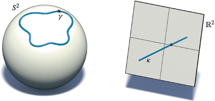

  

  The curvature function $\kappa$ of a curve on $S^2$ lies on a straight line which does not pass through the origin

Proof

Claim (i) is obvious, since the image of a curve lies on a straight line if and only if its unit tangent T is constant. If the image of $\kappa$ lies in a hyperplane through the origin of $\mathbb {R}^{n-1}$, there is a unit vector $\mathbf {a}\in \mathbb {R}^{n-1}$ such that $\langle \mathbf {a},\kappa \rangle =0$. Then

$$\displaystyle \begin{aligned} (N\mathbf{a})'=-\langle \kappa,\mathbf{a}\rangle=0\end{aligned}$$

so there is a fixed vector $\mathbf {n}\in \mathbb {R}^n$ such that $N\mathbf {a}=\mathbf {n}$. We have

$$\displaystyle \begin{aligned} \langle \mathbf{n} ,\gamma\rangle'=\langle N\mathbf{a},T\rangle =0\end{aligned}$$

and therefore the image of $\gamma$ is contained in a hyperplane with normal vector $\mathbf {n}$. The proof of the converse is left to the reader. This establishes (iii). For (iv), suppose that there is a unit vector $\mathbf {a}\in \mathbb {R}^{n-1}$ and a number $r>0$ such that

$$\displaystyle \begin{aligned} \langle \mathbf{a},\kappa\rangle =\frac{1}{r}.\end{aligned}$$

Then

$$\displaystyle \begin{aligned} (\gamma-rN\mathbf{a})'=T-r\langle \kappa,\mathbf{a}\rangle T=0\end{aligned}$$

so there is a fixed point $\mathbf {m}\in \mathbb {R}^n$ such that

$$\displaystyle \begin{aligned} \gamma-rN\mathbf{a}=\mathbf{m}\end{aligned}$$

and we have

$$\displaystyle \begin{aligned} |\gamma-\mathbf{m}|=r.\end{aligned}$$

Therefore, the image of $\gamma$ lies on the hypersphere with center $\mathbf {m}$ and radius r. Again, the proof of the converse is left to the reader and we have established (iv). For (ii) we use induction on n based on (iii), starting at $n=2$ where we use (iv). □