Mixed Strategy Nash Equilibrium

Abstract

In previous chapters, we considered games that had at least one NE, such as the Prisoner’s Dilemma, the Battle of the Sexes, and the Chicken games. But, do all games have at least one NE? If we restrict players to choose a specific strategy with certainty, some games may not have an NE.

Appendices

Appendix—NE Existence Theorem (Technical)

This appendix provides a short proof of the existence of an NE, either in pure or mixed strategies, using Kakutani’s fixed-point theorem. Therefore, we start by introducing the concept of fixed point and two standard fixed-point theorems in the literature.

5.1.1 Fixed-Point Theorems, an Introduction

Consider a function $f:X\rightarrow X$, mapping elements from X into X, where $X\subset \mathbb {R} ^{N}$. We, then, say that a point $x\in X$ is a “fixed point” if $x\in f(x)$. For instance, if $X\subset \mathbb {R}$, we can define the distance function $g(x)=f(x)-x$, which graphically measures the distance from f(x) to the 45-degree line, as illustrated in Fig. 5.8a and b. At points such as $x^{\prime }$ where $g(x^{\prime })>0$, we have that $f(x^{\prime })>x^{\prime }$, meaning that $f(x^{\prime })$ lies above the 45-degree line. In contrast, at points such as $x^{\prime \prime }>x^{\prime }$ where $g(x^{\prime \prime })<0$, we have that $f(x^{\prime \prime })<x^{\prime \prime }$, entailing that $f(x^{\prime \prime })$ lies below the 45-degree line.

Since $x^{\prime \prime }>x^{\prime }$, if distance function g(x) is continuous, we can invoke the intermediate value theorem to say that there must be an intermediate value, $\widehat{x}$, between $x^{\prime }$ and $x^{\prime \prime }$ (or more than one) where $g(\widehat{x})=0$, implying that $g(\widehat{x})=f(\widehat{x})-\widehat{x}=0$, which implies that $f(\widehat{x})=\widehat{x}$, as required for a fixed point to exist.¹⁶ (Note that if f(x) was not continuous, then g(x) would not be continuous either, allowing for $g(x^{\prime })>0$ and $g(x^{\prime \prime })<0$ to occur, yet we could not guarantee the existence of an intermediate point between $x^{\prime }$ and $x^{\prime \prime }$ for which $g(x)=0$.) The Brouwer’s fixed-point theorem formalizes this result.

Fig. 5.8

(a) Function f(x) and the 45-degree line (b)

Definition 5.12. Brouwer’s fixed-point theorem. If $f:X\rightarrow X$ is a continuous function, where $X\subset \mathbb {R} ^{N}$, then it has at least one fixed point, that is, a point $x\in X$ where $f(x)=x$.

While Brouwer’s fixed-point theorem is useful when dealing with best response functions, it does not apply to best response correspondences, where player i is, for instance, indifferent between two or more of her pure strategies when her opponent chooses strategy $s_{j}$. The following theorem generalizes Brouwer’s fixed-point theorem to correspondences. For a more detailed presentation on fixed-point theorems, see Border (1985).

Definition 5.13. Kakutani’s fixed-point theorem. A correspondence $F:X\rightarrow X$, where $X\subset \mathbb {R} ^{N}$, has a fixed point $x\in X$ where $F(x)=x$, if these conditions hold:

• 1. X is a compact, convex, and non-empty set.

• 2. F(x) is non-empty.

• 3. F(x) is convex.

• 4. F(x) has a closed graph.

Nash’s (1950) existence theorem is a direct application of Kakutani’s fixed point theorem, as the next section describes.

5.1.2 Nash Existence Theorem

First, define player i’s pure-strategy set, $S_{i}$, to be finite, i.e., a discrete list of pure strategies, and denote a mixed strategy for this player as $\sigma _{i}$, where $\sigma _{i}\in \sum _{i}$, meaning that player i chooses her randomization among all possible mixed strategies available to her. Therefore, the Cartesian product

$$\begin{aligned} \sum _{i}\times \sum _{-i}=\sum \end{aligned}$$

denotes the set of all possible mixed strategy profiles in the game, so that every strategy profile $\sigma =(\sigma _{i},\sigma _{-i})$ satisfies $\sigma \in \sum$. Second, let us define player i’s best response correspondence to her rivals choosing $\sigma _{-i}$ as $\sigma _{i}\in BR_{i}(\sigma _{-i})$.

We now define the joint best response correspondence $BR(\sigma )$, as the product of $BR_{i}(\sigma _{-i})$ and $BR_{-i}(\sigma _{i})$, that is,

$$\begin{aligned} BR(\sigma )\equiv BR_{i}(\sigma _{-i})\times BR_{-i}(\sigma _{i}). \end{aligned}$$

Importantly, if BR has a fixed point, then, an NE exists. Therefore, we next check if BR satisfies the four conditions on Kakutani’s fixed-point theorem, as that would guarantee the existence of an NE. Before doing that, we identify X in Kakutani’s fixed-point theorem with the set of all possible mixed strategy profiles, $\sum$; and correspondence F with BR.

• 1. $\sum$ is a non-empty, compact, and convex set.

  • (a) The set $\sum$ is non-empty as long as players have some strategies, so we can identify pure or mixed strategy profiles.

  • (b) Recall that if a set is closed and bounded it is compact. The set of all possible mixed strategy profiles is closed and bounded, thus satisfying compactness.

  • (c) Convexity is satisfied since, for any two strategy profiles, $\sigma$ and $\sigma ^{\prime }$, their linear combination, $\lambda \sigma +(1-\lambda )\sigma ^{\prime }$ where $\lambda \in \left[ 0,1\right]$, is also a mixed strategy profile, thus being part of $\sum$.

• 2. $BR(\sigma )$ is non-empty. Since every player i’s payoff, $u_{i}(\sigma _{i},\sigma _{-i})$, is linear in both $\sigma _{i}$ and $\sigma _{-i}$, she must find a maximum (a best response to her rivals choosing $\sigma _{-i}$) among her available strategies, $\sum _{i}$, which we know it is a compact set from point 1b. Because $\sigma _{i}\in BR_{i}(\sigma _{-i})$ and $\sigma _{-i}\in BR_{i}(\sigma _{i})$ are non-empty (a best response exists), then their product, $BR(\sigma )$, must also be non-empty.

• 3. $BR(\sigma )$ is convex. To prove this point, consider two strategies for player i, $\sigma _{i}$ and $\sigma _{i}^{\prime }$, that are best responses to her rivals choosing $\sigma _{-i}$, that is, $\sigma _{i},\sigma _{i}^{\prime }\in BR_{i}(\sigma _{-i})$. Because both $\sigma _{i}$ and $\sigma _{i}^{\prime }$ are best responses, they must both yield the same expected payoff; otherwise, one of them cannot be a best response. Therefore, a linear combination of $\sigma _{i}$ and $\sigma _{i}^{\prime }$, $\lambda \sigma _{i}+(1-\lambda )\sigma _{i}^{\prime }$ where $\lambda \in \left[ 0,1\right]$, must yield the same expected payoff as $\sigma _{i}$ and $\sigma _{i}^{\prime }$, thus being a best response as well, that is, $\lambda \sigma _{i}+(1-\lambda )\sigma _{i}^{\prime }\in BR_{i}(\sigma _{-i})$.

  Alternatively, this result can be proven by contradiction. Consider strategies $\sigma _{i}$ and $\sigma _{i}^{\prime }$, both being best responses to $\sigma _{-i}$, that is, $\sigma _{i},\sigma _{i}^{\prime }\in BR_{i}(\sigma _{-i})$; but suppose that strategy $\sigma _{i}^{\prime \prime }=\lambda \sigma _{i}+(1-\lambda )\sigma _{i}^{\prime }$ is not a best response. In particular, assume that there is a value of $\lambda \in \left[ 0,1\right]$ for which strategy $\sigma _{i}^{\prime \prime }$ yields a strictly higher payoff than $\sigma _{i}$ and $\sigma _{i}^{\prime }$. Then, $\sigma _{i}^{\prime \prime }$ must be a best response to $\sigma _{-i}$, i.e., $\sigma _{i}^{\prime \prime }\in BR_{i}(\sigma _{-i})$. This result, however, contradicts our premise that strategies $\sigma _{i}$ and $\sigma _{i}^{\prime }$ are best responses to $\sigma _{-i}$. Therefore, if strategies $\sigma _{i}$ and $\sigma _{i}^{\prime }$ are best responses to $\sigma _{-i}$, their linear combination $\sigma _{i}^{\prime \prime }=\lambda \sigma _{i}+(1-\lambda )\sigma _{i}^{\prime }$ is a best response to $\sigma _{-i}$ as well.

• 4. $BR(\sigma )$ has a closed graph. This property states that the set $\left\{ (\sigma _{i},\sigma _{-i})|\sigma _{i}\in BR_{i}(\sigma _{-i})\right\}$ is “closed,” meaning that every player i’s best response correspondence has no discontinuities. The best responses depicted in this chapter, for instance, showed no discontinuities. Because every player i’s payoff, $u_{i}(\sigma _{i},\sigma _{-i})$, is continuous and compact, the set $\left\{ (\sigma _{i},\sigma _{-i})|\sigma _{i}\in BR_{i}(\sigma _{-i})\right\}$ is closed.

The previous result guarantees that an NE exists when players face finite strategy spaces (i.e., a list of pure strategies). What if players choose from a continuous strategy space, as when firms set their prices or output levels? Glicksberg (1952) extended the above result to settings with continuous strategy spaces, where $S_{i}\subset \mathbb {R} ^{N}$, showing that, if every player i’s strategy space, $S_{i}$, is compact and her utility function, $u_{i}(\cdot )$, is continuous, an NE exists, in pure or mixed strategies. (For a generalization of this result to non-continuous utility functions, see Dasgupta and Maskin (1986).)

Exercises

• 5.1 General Battle of the Sexes game.$^{A}$ Consider the following Battle of the Sexes game where every player simultaneously chooses between going to the football game (F) or the opera (O). Payoffs satisfy $a_{i}>b_{i}>0$ for every player $i=\{H,W\}$, implying that the husband (Wife) prefers that both players are together at the football game (opera house, respectively), and attending any event is preferred to being alone anywhere. However, the premium that player i assigns to his or her most preferred event, as captured by $a_{i}-b_{i}$, can be different between husband and wife.

  

  • (a) Find the msNE of this game.

  • (b) How are players’ randomization affected by an increase in payoffs $a_{H}$, $a_{W}$, $b_{H}$, and $b_{W}\,$? Interpret.

  • (c) How are your results affected if the husband earns a larger payoff from the football game than his wife earns from the opera, $a_{H}>a_{W}$? How are your findings affected otherwise?

• 5.2 General Pareto coordination game.$^{A}$ Consider the following Pareto coordination game where every firm simultaneously choosing between technology A or B, and payoffs satisfy $a_{i}>b_{i}>0$ for every firm $i=\{1,2\}$, implying that both firms regard technology A as superior. However, the premium that firm i assigns to technology A, as captured by $a_{i}-b_{i}$, can be different between firms 1 and 2.

  

  • (a) Find the msNE of this game.

  • (b) How are players’ randomization affected by an increase in payoffs $a_{1}$, $a_{2}$, $b_{1}$, and $b_{2}\,$? Interpret.

  • (c) How are your results affected if firm 1 earns a larger payoff from technology A than firm 2 does, $a_{1}>a_{2}$? How are your findings affected otherwise?

• 5.3 General anticoordination game.$^{A}$ Consider the following Game of Chicken where every player drives toward each other and simultaneously chooses between swerve and stay. Payoffs satisfy $a_{i}>b_{i}>0$ for every player $i=\{1,2\}$, implying that drivers suffer more when they both stay (and almost die!) than when they both swerve (and are called chickens), and $a_{i}>d_{i}>c_{i}>b_{i}$, so being the only player who stays yields a payoff of $d_{i}$ for that player and $-c_{j}$ for his rival, where $j\ne i$.

  

  • (a) Find the msNE of this game.

  • (b) How are players’ randomization affected by an increase in payoffs $a_{1}$ through $d_{1}$? How are they affected by a marginal increase in $a_{2}$ through $d_{2}$? Interpret.

• 5.4 Asymmetric Matching Pennies game.$^{A}$ Consider the following Matching Pennies game where every player simultaneously chooses Heads (H) or Tails (T) and payoff a satisfies $a>0$.

  

  • (a) Find the msNE of this game.

  • (b) How are the equilibrium probabilities of each player affected by an increase in payoff a? Interpret your results.

• 5.5 Anticoordination in the Stop–Go game.$^{A}$ Consider the following anticoordination game where two drivers meet at a road intersection. Each driver i chooses to stop (waiting for the other driver to continue) or to go (not waiting for the other driver). Parameter c denotes the cost of stopping while the other driver goes, where $1>c>0$. If both drivers stop, they both earn 1; if they both go, they crash their cars, earning zero; and if driver i stops while his opponent goes, driver i earns $1-c$ while his opponent earns 3.

  

  • (a) Find the best responses of each driver.

  • (b) Find the psNEs of this game.

  • (c) Find the msNE of this game.

• 5.6 Anticoordination in the job application game.$^{A}$ Consider two college students applying for a job at either of the two companies (A or B). Firm B offers a more attractive salary than firm A, $w_{B}>w_{A}$, but both students working for firm A would be better-off than only one of them working for firm B, that is, $2w_{A}>w_{B}$. Every student simultaneously and independently applies for a job to one, and only one, company. If only one student applies to a firm, he gets the job. If both apply to the same firm, each of them gets the job with probability of 1/2.

  • (a) Depict the game’s payoff matrix.

  • (b) Find the best responses of each player.

  • (c) Find the psNEs of this game.

  • (d) Find the msNE of this game.

  • (e) How are your equilibrium results in the msNE affected by a marginal increase in $w_{A}$? And by a marginal increase in $w_{B}$? Interpret.

• 5.7 Finding msNE in the salesman’s game.$^{B}$ Consider a salesman who, after returning from a business trip, can be honest about his expenses (H) or lie about them (L) claiming more expenses than he actually had. His boss can either not check the salesman (NC) or check whether his claimed expenses are legit (C). If the salesman is honest, he is reimbursed for his expenses during the trip, entailing a payoff of zero for him, and a payoff of zero for his boss when he does not check on the salesman but $-c$ otherwise (we can interpret c as the cost that the boss incurs when checking). If the salesman lies, he earns $a>0$ when his boss does not check on him, but when he does, the salesman’s payoff is $-b$ from his boss detects his cheating (which occurs with probability p) and a when his boss does not detect his cheating (which happens with probability $1-p$). If the boss checks when the salesman lies, the boss’ payoff is $-c+\left[ p0+(1-p)\left( -\beta \right) \right] =-c-(1-p)\beta$, which embodies his (certain) cost from checking and his expected cost of not detecting the lie, which occurs with probability $1-p$.

  • (a) Depict the game’s payoff matrix.

  • (b) Find the best responses of each player.

  • (c) Find the psNEs of this game.

  • (d) Find the msNE of this game.

• 5.8 Quantal Response Equilibrium—An introduction.$^{C}$ Consider again the asymmetric Matching Pennies game. Luce (1959) suggests that every player $i=\{1,2\}$ chooses Heads based on its “intensity,” defined as follows

  $$\begin{aligned} \sigma _{iH}=\frac{u_{iH}}{u_{iH}+u_{iT}} \end{aligned}$$

  where $u_{iH}$ denotes player i’s utility from choosing H, while $u_{iT}$ represents his utility from selecting T. A similar intensity applies to his probability of playing Tails, $\sigma _{iT}=\frac{u_{iT}}{u_{iH}+u_{iT}}$, which satisfies $\sigma _{iT}=1-\sigma _{iH}$.

  • (a) Show that, in the asymmetric matching pennies game, utilities $u_{iH}$ and $u_{iT}$ are themselves functions of probabilities $\sigma _{iH}$ and $\sigma _{iT}$.

  • (b) Find the equilibrium probabilities $\sigma _{iH}^{QRE}$ and $\sigma _{iT}^{QRE}$, where the superscript QRE denotes “quantal response equilibrium.”

  • (c) How are the equilibrium probabilities of each player affected by an increase in payoff a? Interpret your results.

  • (d) Compare $\sigma _{iH}^{QRE}$ and $\sigma _{iT}^{QRE}$ against the mixed strategy equilibrium, $\sigma _{iH}^{*}$ and $\sigma _{iT}^{*}$, found in the previous exercise.

  • (e) Consider now that the intensity function is

    $$\begin{aligned} \sigma _{iH}=\frac{\left( u_{iH}\right) ^{\lambda }}{\left( u_{iH}\right) ^{\lambda }+\left( u_{iT}\right) ^{\lambda }} \end{aligned}$$

    where $\lambda \ge 0$ is known as the responsiveness or precision parameter. Find the equilibrium probabilities in this context. Then, evaluate your results at $\lambda =0$, showing that strategy H is unresponsive to expected payoffs, implying that players mix between H and T with equal probability. Finally, evaluate your results at $\lambda =4$, and interpret your findings.

• 5.9 Stag Hunt game.$^{B}$ Consider the following Stag Hunt Game where two individuals simultaneously choose between hunt a stag or a hare. Payoffs satisfy $a_{i}>b_{i}>d_{i}>c_{i}$ for every player i, so every player’s ranking of payoffs is: (1) hunting a stag with the help of his opponent; (2) hunting a hare with the help of his opponent; (3) hunting a stag without help; and (4) hunting a hare without help.

  

  • (a) Find the msNE of this game.

  • (b) How are players’ randomization affected by an increase in payoffs $a_{1}$ through $d_{1}$? Interpret.

• 5.10 Finding msNEs in four categories of simultaneous-move games.$^{B}$ Consider the following simultaneous-move game with payoff matrix

  

  Find the msNE in the following settings. Interpret and relate your results to common games.

  • (a) Payoffs satisfy $a>c$ and $b>d$.

  • (b) Payoffs satisfy $a>c$ and $b<d$.

  • (c) Payoffs satisfy $a<c$ and $b<d$.

  • (d) Payoffs satisfy $a<c$ and $b>d$.

  • (e) In the setting of part (d), discuss how your results are affected if the difference $b-d$ increases. What if the difference $c-a$ increases? Interpret.

• 5.11 Mixed strategies do not assign probability to dominated pure strategies.$^{B}$ Consider the following Prisoner’s Dilemma game between players 1 and 2.

  

  Assume that player i randomizes with a mixed strategy $\sigma _{i}$ that puts positive probability on Not Confess, despite being strictly dominated.

  • (a) Find the probability of player j, q, that makes player i indifferent between Confess and Not Confess. Show that probability q would satisfy $q\notin \left( 0,1\right)$. Interpret.

  • (b) Let us now take a more general approach. Consider a two-player game (not necessarily the Prisoner’s Dilemma game) where player i randomizes with a mixed strategy $\sigma _{i}$ that puts positive probability on a strictly dominated strategy. Show that $\sigma _{i}$ is dominated by another mixed strategy $\sigma _{i}^{\prime }$ that puts zero probability weight on a strictly dominated strategy. For generally, let player i have L pure strategies $S_{i}=\{s_{i1},...,s_{iL}\}$ and let $s_{ik}$ be a pure strategy which is strictly dominated by $s_{ik^{\prime }}$, that is, $u_{i}(s_{ik^{\prime }},s_{-i})>u_{i}(s_{ik},s_{-i})$ for every $s_{-i}$.

• 5.12 Pure and mixed NEs with weakly dominant strategies.$^{A}$ Consider the payoff matrix in Exercise 2.4 again.

  • (a) Find all pure-strategy Nash equilibrium of this game.

  • (b) Can you identify a mixed strategy Nash equilibrium? Explain.

  • (c) Characterize and plot the best response functions you found in part (c). Interpret.

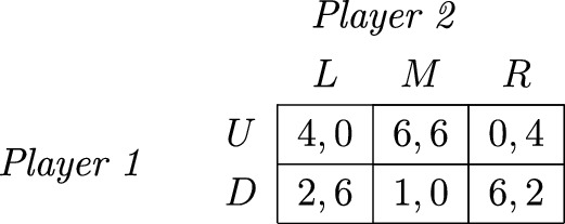
• 5.13 Finding msNEs in a general game.$^{B}$ Consider the following two-player game, based on Fudenberg and Tirole (1991, page 480). Answer the following questions allowing for psNEs and msNEs.

  

  • (a) If $0<a<1\,$and $b\le 0$, show that the game has one psNE, and find the condition for msNE.

  • (b) If $a=0\,$and $b<0$, show that the game has only one NE.

  • (c) If $a=0\,$and $b>0$, show that the game has three NEs.

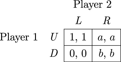
• 5.14 Small perturbations and NE.$^{B}$ Consider the following two-player game.

  

  • (a) Find the set of psNE and msNE.

  • (b) If both players’ payoffs in (U, L), at the top left cell of the matrix, increase from 1 to $1+\varepsilon$, where $\varepsilon >0$, how are your results in part (a) affected?

  • (c) How does your answer to part (b) change if, instead, $\varepsilon <0$?

• 5.15 IDSDS, NE, and security strategies.$^{B}$ Consider the following simultaneous-move game where player 1, in rows, chooses A, B, or C; while player 2, in columns, chooses between a and b.

  

  • (a) Does player 1 or 2 have a strictly dominated strategy? What about weakly dominated strategies?

  • (b) Find the strategy profile/s surviving IDSDS. Find the strategy profile/s surviving IDWDS.

  • (c) Find player 1’s best responses to each of player 2’s strategies. Then, find player 2’s best responses to each of player 1’s strategies.

  • (d) Find the psNEs of this game.

  • (e) Find the security strategy profile (maxmin) of this game.

  • (f) Compare your equilibrium results according to IDSDS and IDWDS (from part b), psNE (from part d), and security strategies (from part e). Interpret your results.

• 5.16 Trembling-hand perfect equilibrium—Examples.$^{B}$ Consider the following payoff matrix.

  

  • (a) Find all pure-strategy NEs of this game.

  • (b) Show that only one of the NEs found in part (a) can be supported as a THPE.

• 5.17 Trembling-hand perfect equilibrium-Proofs.$^{C}$ Show that:

  • (a) Every THPE must be an NE.

  • (b) Every strategic-form game with finite strategies for each player has a THPE.

  • (c) Every THPE assigns zero probability weight on weakly dominated strategies.

• 5.18 Proper equilibrium—Example.$^{B}$ Consider the Hawk–Dove game in the matrix below (an example of an anticoordination game), where player 1 chooses between Hawk and Dove in rows (H or D), and player 2 chooses between these two pure strategies in columns (h and d).

  

  • (a) Find the pure-strategy NEs in this game.

  • (b) Check with of the NEs found in part (a) are proper.

• 5.19 Finding msNE and security strategies with players have three available actions.$^{B}$ Consider the simultaneous-move game between players 1 and 2 in the following payoff matrix.

  

  • (a) Find the NEs involving pure strategies.

  • (b) Find the msNE of this game.

  • (c) Find the security strategies of this game.

References

Aumann, R. (1974) “Subjectivity and Correlation in Randomized Strategies,” Journal of Mathematical Economics, 1(1), pp. 67–96.
Border, K. C. (1985) Fixed Point Theorems with Applications to Economics and Game Theory, Cambridge University Press, Cambridge.
Dasgupta, P., and E. Maskin (1986) “The Existence of Equilibrium in Discontinuous Economic Games, II: Applications,” Review of Economic Studies, 46, pp. 27–41.
Fudenberg, D., and J. Tirole (1991) Game Theory, The MIT Press, Cambridge, Massachussets.
Glicksberg, I. L. (1952) “A Further Generalization of the Kakutani Fixed Point Theorem with Application to Nash Equilibrium Points,” Proceedings of the National Academy of Sciences, 38, pp. 170–174.
Harsanyi, J.C. (1973) “Oddness of the Number of Equilibrium Points: A New Proof,” International Journal of Game Theory, 2, pp. 235–250.
Luce, R. D. (1959) Individual Choice Behavior, John Wiley, New York.
Myerson, R. (1978) “Refinements of the Nash Equilibrium Concept,” International Journal of Game Theory, 7, pp. 73–80.
Selten, R. (1975) “Reexamination of the Perfectness Concept for Equilibrium Points in Extensive Games,” International Journal of Game Theory, 4, pp. 301–324.
Von Neumann, J. (1928) “Zur Theorie der Gesellschaftsspiele,” Mathematische Annalen, 100, pp. 295–320.
Watson, J. (2013) Strategy: An Introduction to Game Theory, Worth Publishers. Third edition.
Wilson, R. (1971) “Computing Equilibria in N-person Games,” SIAM Journal of Applied Mathematics, 21, pp. 80–87.
Author information
Authors and Affiliations
Corresponding author