
Abstract
We present an overview of recent developments in the area of acoustic sensing that is inspired by biology and realized by micro-electromechanical systems (MEMS). To support understanding, an overview of the principles of human hearing is presented first. After the review of bio-inspired sensing systems, we continue with an outline of an adaptable acoustic MEMS-based sensor that offers adaptable sensing properties due to a simple, real-time feedback. The transducer itself is based on an active cantilever, which offers the advantage of an integrated deflection sensing based on piezoresistive elements and an integrated actuation using thermomechanical effects. We use a feedback loop, which is realized via a field-programmable gate array or analog circuits, to tune the dynamics of the sensor system. Thereby, the transfer characteristics can be switched between active, linear mode, for which the sensitivity and minimal detectable sound pressure level can be set by the feedback strength (similar to control of the quality factor), and an active nonlinear mode with compressive characteristics. The presented sensing system, which is discussed both from an experimental and theoretical point of view, offers real-time control for adaptation to different environments and application-specific sound detection with either linear or nonlinear characteristics.
You have full access to this open access chapter, Download chapter PDF
Keywords
- Bio-inspired acoustic sensing
- Micro-electromechanical system (MEMS)
- Mathematical modelling
- Real-time feedback
- Adaptative sensing
1 Introduction
Current technological sound and speech processing systems typically consist mainly of three parts (schematically shown in Fig. 1): a sensing unit, a pre-processing unit and the sound analysis/processing unit. The sensing unit consists of one or more (typically capacitive) microphone based on micro-electro-mechanical system (MEMS)-technology with linear transfer characteristics and 120 dBA as maximal detectable sound pressure level (SPL), a self-noise floor (corresponding to the minimal detectable SPL) of \(20-30\) dB (absolute minimum at the moment (non-MEMS): \(\approx 7\) dB), and a frequency range of 20 Hz-20 kHz [1]. The pre-processing unit is applied to tune the sensed signals for easier processing/analysis. It typically includes a pre-amplifier, amplifying the microphones signals, and filter stages, decomposing the signal into different frequency bands, and additional stages to include e.g. weighting functions, correcting the signal and/or digitalizing it. The processing unit is based on signal processing stages and/or on learning systems such as convolutional, recurrent and spiking neural networks. Thereby, the pre-processing of the signals shall improve the processing performance by extracting important sound features, which are then fed into the neural networks (see e.g. [2]). Typical low-complexity features are, for example, the envelope of the sound signal, the RMS energy, the frequency (given by the zero crossing rate or the spectral centroid) or spectral spread or flux. Alternatively, the sound data is fed directly into the NN, known as end-to-end learning, or first transformed into a time-frequency representation, known as spectrogram, before it is fed into the network. The goal is to separate the relevant information like speech from irrelevant one like noise.
The performance of speech processing systems has strongly increased in recent years [3,4,5,6,7]. This can be mainly attributed to the improvements in the pre-processing stage and the sound processing networks, since microphone technology including readout is well developed with easy and cheap fabrication, small size and large dynamic ranges and performance. The pre-processing stage typically includes pre-amplifiers, amplifying the microphone signals, and filter stages, decomposing the signal into different frequency bands, and additional stages to include, e.g., weighting functions, correct and/or digitalize the signal. The development of pre-processing stage was driven mainly by implementing bio-inspired pre-processing (e.g. nonlinear amplification) as well as developing extensive noise cancellation algorithms. Thereby, it was recently shown that nonlinear, bio-inspired pre-processing based on frequency filtering and nonlinear amplification of signals is particularly important for sound processing, since it yields strongly increased success rates for speech classification tasks [8]. The increasing demands in computation power and energy can be addressed by neuromorphic, bio-inspired pre-processing implementations in hardware like silicon cochlea, Hopkins electronic ear, AER-EAR, or the FPGA cochlea [9]. These model sound processing by the cochlea in the inner ear, as schematically shown in Fig. 1 and, compared to software implementations, offer the advantage of low latency, real-time performance, reduction of redundant information and data streaming (due to asynchronous event-based spiking output) and lower power consumption. Noise cancellation algorithms can be applied to improve sound processing in more complex hearing situations with multiple sources, but these increase the necessary computing power and energy consumption. In both cases, the idea is to improve the sound feature representation in the audio signals to allow a better sound processing in the neural networks.

Comparison of steps in technological speech processing systems and the human hearing system. Detailed description of human hearing is given in chapter 2. BM-basilar membrane, OHC-outer hair cell, IHC-inner hair cell, AN-auditor nerve
Despite these developments, room reverberation (echos), interfering noise, or any other perturbation to the signal can critically affect the underlying feature representation and thus limit sound processing performance, in particular, at low signal-to-noise ratios (SNRs) [10,11,12]. Further challenges arise from the inability to separate individual sound sources from a mixed acoustic signal, to generalize to unknown acoustic conditions, and to run on low-power embedded devices. Adaptation of the system parameters can help to overcome the issues arising from changing acoustic environments such as room reverberations, noise level etc. Current research focused on adaptation of the pre-processing stage: changing the gain of the pre-amplifier [13], the settings of the filter banks [14], how signals are combined for improved directionality [15], microphone switching to increase dynamic range [16] or automatic gain control in neuromorphic systems [17, 18]. Although methods to adapt the sensing properties of microphones have been published, e.g., adjusting sensitivity by changing the bias voltage or effective microphone area [19], these are not (widely) applied. While the above described developments could improve sound processing performance for standard hearing conditions (combined with higher computing power demands), until now satisfying solutions for reasonable sound processing of signals in noisy environments, i.e., with low signal-to-noise ratios, low volume of important sounds or loud masking sounds, could not be derived.
Thus, improving the sensor stage is the next logical step to bridge this gap. In this chapter we will review (some of) the research in bio-inspired acoustic sensors. For a better understanding, we will shortly summarize what is known about the acoustic sensing in humans until the transduction stage, including the processing and encoding mechanisms occurring at this level. Following this, several bio-inspired sensors will be described in relation to their processing capabilities, in particular frequency decomposition and nonlinear filtering of the sound signals, and their adaptation properties, which are the most important functionalities in acoustic bio-inspired sensing. Finally, we will present a bio-inspired acoustic sensor [20,21,22] that includes all the above mentioned three functionalities, i.e. frequency decomposition, nonlinear amplification and adaptation.
2 Human Hearing/Auditory Pathway
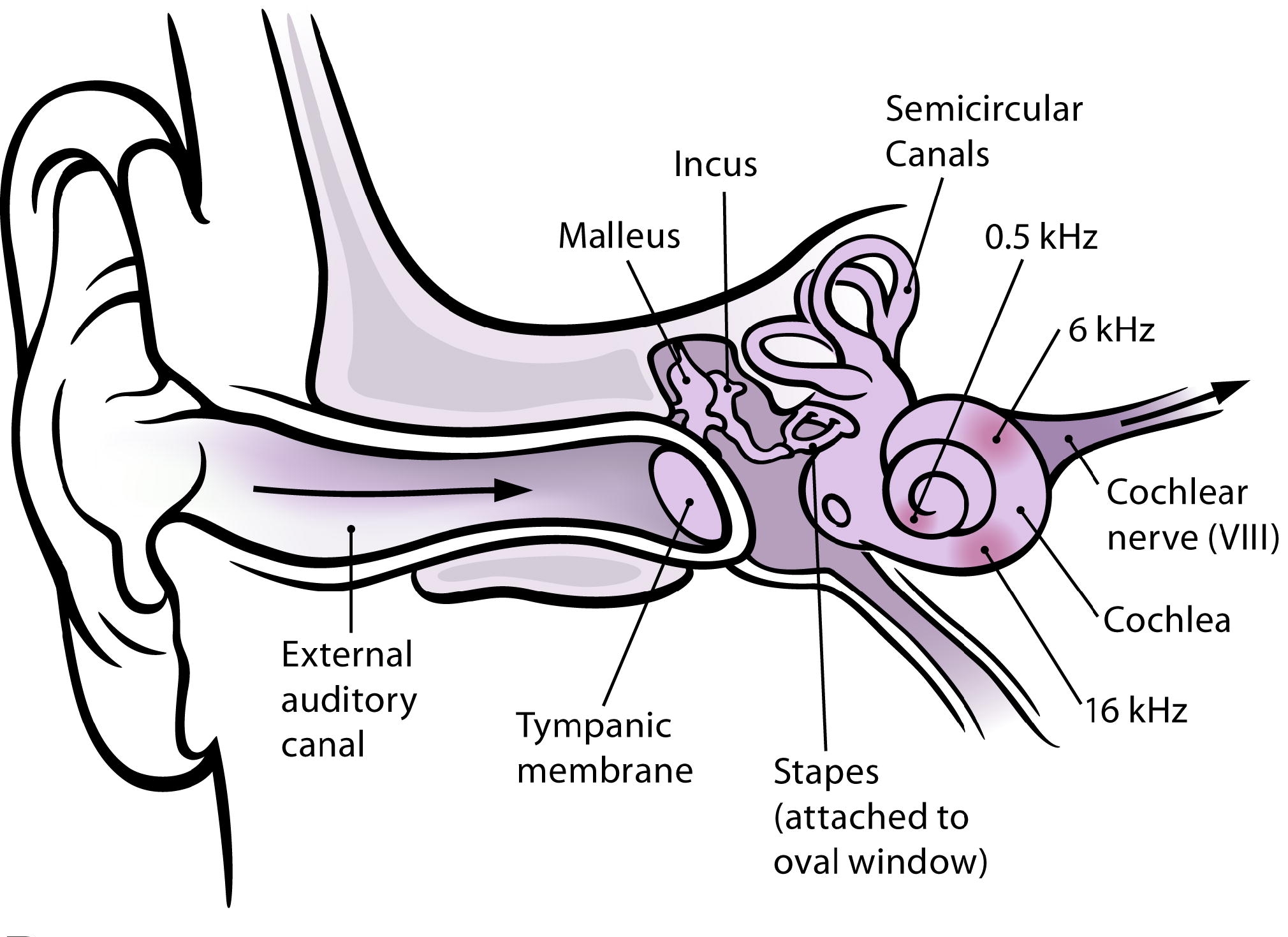
In this section, we will give a short overview of the hearing process until the transduction of acoustic signals with a particular focus on the pre-processing of the signal taking place before the actual sound analysis in the cortex (see Fig. 1). The description is mainly based on the information given in [23, 24] and is separated according to the three parts of the ear (see Fig. 2): (i) the outer ear, which includes the pinna and the external auditory canal, (ii) the middle ear with the ossicular chain consisting of incus, malleus and stapes, and (iii) the inner ear with the cochlea.

Modified from [25]
Schematic illustration of the ear.
Human hearing starts with the pinna, which funnels the sound signals into the ear canal, further transferring the signal to the tympanic membrane. Even in this very first step of the hearing process, several steps before the actual transduction of sound signals into electric signals (action potentials/spikes), a pre-processing/conditioning of the acoustic signals is present, which shall support later sound processing and sound perception. In detail, the transfer characteristics of the outer ear pinna and ear canal is on the one hand direction-dependent, providing localization cues, and on the other hand includes frequency-selective amplification of sound signals. The latter amplifies the sound signals in the important range of 200Hz to 10kHz, with particularly strong amplification in the range of 2-4kHz, the range of highest sensitivity for hearing [26]. This pre-conditioning is mainly constant and not adaptive.
In the next step of the hearing process, the vibrations of the tympanic membrane due to sound excitation are transferred to the inner ear by the ossicular chain in the middle ear. Its task is to provide an impedance matching between the air-based sound in the outer ear and the fluid-based sound propagation in the inner ear. Without this matching, most of the sound energy would be reflected at the air-fluid interface whith a reflectance of approximately 99.9%. The transfer characteristics is almost flat in the range between 200Hz and 8kHz (small peaks around 1kHz-2kHz and 4-5kHz) and decreases outside this range. Important to note here is that the efficiency of sound transfer can be adapted for small frequencies below 2 kHz by contraction of the stapedius muscle. Its contraction yields an increase of the stiffness of the ossicular chain , thus reducing the sound energy transferred to the inner ear. The main purpose of this adaptation is a protection of the inner ear from damage due to loud noises and an attenuation of the perception of ones own voice.

From [27]
Schematic showing the cross-section of the cochlea with focus on the organ-of-corti, which is the place of sound transduction. Thereby, the organ of corti is located in the the scala media, one of the three fluid-filler chambers of the cochlea with scala tympani below and scala vestibuli above. The three chambers are separated by Reissner’s membrane on top and basilar membrane below, which hosts the organ of corti.
The final part in the acoustic sensing process is the inner ear, the cochlea to be accurate. The cochlea itself, a bony, snail shell-resembling structure consists of three fluid-filled chambers: the scala vestibuli, the scala tympani and between both the scala media, hosting the organ of corti (see Fig. 3). Thereby, the scala vestibuli is separated from the scala media by a thin membrane, the Reissner’s membrane. On the lower side, scale media is separated from the scale tympani by the basilar membrane (BM).
The pressure wave, initiated by the stapes at the oval window of the cochlea, propagates through the scala tympani up to the apex of the cochlea, where it is transferred to the scale vestibuli through a small connection of both chambers and then propagates in this chamber down to the base of the cochlea until finally reaching the round window (see Fig. 4). In response to the propagating sound wave, the basilar membrane and Reissners membrane oscillate. Thereby, due to a varying stiffness and thickness of the basilar membrane along the cochlea length, resonance occurs at different locations in the cochlea depending on the frequency of the sound wave (traveling wave theory), yielding an effective frequency decomposition of the input signal. This encoding of sound frequency into a location/place along the cochlea is termed tonotopy and the frequency-place coding is kept throughout the complete auditory pathway up to the auditory cortex in the brain. Thereby, humans can distinguish frequencies differing only by 0.1% [28]. The sharpness of the frequency resolution and cochlear sensitivity is discussed to be further influenced by the longitudinal variation in stiffness of the tectorial membrane (TM) [29].

From [30]
Schematic of a traveling wave propagation in the cochlea.
Situated on the basilar membrane and connected on top with the tectorial membrane in the scala media is the organ of corti (OoC), which hosts the actual acoustic transducers/receptors of human hearing, namely the hair cells. These are cells with cilia on top, giving them their name. In the inner ear, there are two types of hair cells, the inner hair cells (IHC) and the outer hair cells (OHC), with different functionalities, morphology and purpose [23, 31]. Both of them have three rows of differently sized cilia on top, whereby these are V or W-shaped on top of outer hair cells and in a straight line for inner hair cells.
The inner hair cells perform the acoustic sensing/transduction in the following way. The sound pressure wave deflects the cilia on top of the inner hair cell. If the cilia are bent towards the largest ones, potassium channels on top of the cell open. The potassium influx thus polarizes the hair cell and triggers the opening of calcium channels at the bottom. This in turn initiates the release of neurotransmitter glutamate into the synapse between hair cell and acoustic nerve. Glutamate then activates the connected acoustic nerve, yielding to an increase of its spike rate. If cilia are unbend/not deflected, a part of the potassium channels is open, which yields a constant small neurotransmitter release and a constant spiking of the acoustic nerve cell. If the cilia are bent into the other direction, i.e., towards the smallest cilia, (during the second half of the sound sine wave) potassium channels close, calcium channels close and no neurotransmitter is released. This yields a reduction of spike rate at the acoustic nerve. Thus, the sound pressure changes are transformed into the changes of the spike rate at the acoustic nerve (electrical signal).
Here, additional encoding of sound information takes place, in particular of sound amplitude, sound frequency and time course of sound signals, as summarized in Table 1.
The above described phase locking of polarization/hyperpolarisation of the hair cell with the sound input is possible only up to frequencies in the range of 2kHz. The phase locking is another encoding of sound frequency, additional to the frequency-place code discussed above. For frequencies larger than 2kHz, the alternating component of the hair cell potential decreases while the DC component, also termed direct component, increases due to incomplete repolarisation of the cell. In response to this, the spike rate on the auditory nerve will increase strongly at first, but then decrease fast and settle at a certain plateau value in response to a constant pure tone input (see Fig. 5). This is termed rapid and short-term adaptation and can be modelled using e.g. exponential and power-law adaptation [32]. At the offset of the sound input, the spiking rate is strongly reduced below the spontaneous spiking rate (even up to cessation) and slowly recovers to the spontaneous spiking rate. Besides the duration of the stimuli, the adaptation behaviour depends on previous stimuli, sound amplitude, previous stimulation history, and the spontaneous rate of the fibre [33, 34], making it rather complex for modeling. The mechanism underlying the adaptation process is not completely understood. Discussed reasons are the depletion of neurotransmitter or the desensitization of post-synaptic receptors (see e.g. [35, 36]). Whether this adaptation is important for the sound processing is unclear. A discussed functional relevance of this adaptation is the shaping of the onset response, highlighting the sound onset and offset, which might be important, e.g., for time-of-arrival detection used in localisation.

Furthermore, the amplitude of the sound is encoded in the spike rate in three different ways. First, for a single fibre of the auditory nerve, the spike rate depends nonlinear (sigmoidal) on the amplitude of the receptor (hair cell) potential, i.e., for potentials below and above a certain threshold the spiking rate is constant and in between these thresholds a correlation between spike rate and amplitude is observed. The range between thresholds is small compared to the dynamic range of hearing, but enables a high resolution of amplitude encoding. To cover a larger dynamic range, multiple fibres with different sensitivities (from low over medium to high) are connected to one IHC. The combination of their spike rates in response to a sound enables the encoding of a larger amplitude range. For low volume sounds, only the highly sensitive fibres are encoding the sound amplitude. For larger sound levels, the high sensitivity fibres enter the saturation regime (higher threshold), while the medium fibres cross their lower threshold, thus encoding the amplitude of the stimulus. For even higher sound levels, medium sensitivity fibres saturate and low sensitivity fibres can encode the amplitude. For very large sound levels, the region of activated sound fibres becomes much larger then expected from the characteristic frequency. In this case, also the number of activated fibres (size of activated area) encodes the sound amplitude. This combination of different sensitivities helps to encode a large dynamic range.
Nevertheless, the hair cell has to respond to a large range of amplitudes (120 dB) and sound pressure levels (SPL). For the lower SPL, only sub-nm deflections of cilia are generated and the energy of the sound wave exhibits energy levels in the range of thermal noise [37, 38]. Reliable sensing of low SPLs and the large dynamic range would not be possible for purely linear sensors. Here another effect enables the large amplitude range, namely a compressive (nonlinear) amplification before the transduction. Thereby, two mechanisms are discussed as main source for the nonlinear amplification, which are hair bundle motility and somatic motility of outer hair cells [39]. The hair bundle is the group of cilia on top of a hair cell. These are linked by filaments, called tip-links. If these tip-links are stretched, potassium channels open (starting the activation of the hair cell+ auditory nerve). An adaptation mechanism was proposed, which yields a downward movement of the plate of the tip link and thus a reduction in its stretching upon a constant force. This creates a region of negative stiffness in the otherwise linear force-displacement relationship [24]. Due to the nonlinear relationship, the hair bundle dynamics are nonlinear as well, including nonlinear dynamics effects like bifurcation to self-excited oscillations etc. The second discussed effect is somatic motility [40], which is a stretching and compressing movement of the outer hair cell, changing its length. For reviews, see [31, 39, 41]. Here, the influx of potassium (after deflection-induced channel opening) results in the dislocation of chloride ions from prestin molecule. Prestin is a molecule abundant in the OHC membrane, which changes its shape depending on the voltage due to the insertion or removal of chloride ions. If chloride ions leave the prestin molecule, it compresses, which yields a compression of the outer hair cell. This happens when the basilar membrane moves upwards (towards the tectorial membrane). Since the outer hair cell is connected to both (TM and BM), the compression of the OHC yields an amplification of the upward BM motion, i.e. an amplification of the sound input. For the other case, i.e., BM moves downwards (away from TM), potassium channels of OHC close, resulting in the returning of chloride ions into the prestin molecule, which in turn stretches. Thus, the OHC stretches and amplifies the downward motion of the BM.
Besides mammalians, only birds, crocodiles, frogs and lizards have two types of hair cells, whereby only for mammals one might be capable of somatic motility [40, 42, 43]. Nevertheless, amphibians and reptiles like frogs, turtles, and lizards exhibit nonlinear dynamics in the hearing process as well [44,45,46,47,48,49]. Therefore, it was proposed [24, 43, 50, 51], that the hair bundle motility is the reason for the nonlinear amplification but has a low gain of a factor of ten, while somatic motility is intrinsically linear but offers an additional amplification (driven by hair bundle motility) to reach the amplification factor of 1000 observed in mammals.
Besides the frequency decomposition, nonlinear amplification and short-term adaptation described above, further pre-conditioning of the signals occurs in the inner ear, driven by an efferent feedback from subsequent processing stages [52,53,54,55]. This feedback is proposed to control OHC motility by a calcium driven motility. It is expected to be used to reduce unwanted/unattended (non-relevant) contributions in the sound signal by damping the amplification of OHCs. The efferent feedback controls thereby a larger group of OHCs simultaneously (as seen from innervation), but can address specific frequency ranges individually. The efferent feedback was shown to improve speech perception in particular in noisy environments. It is discussed that this improved perception is achieved by the active damping (or the lack of active amplification) for the noisy frequency bands in comparison to the amplification of the frequency bands associated with speech (or important sounds).
Concluding, in the hearing process up to transduction of the signal into electrical signals, a number of pre-processing steps are involved, which are thought to improve sound/speech perception and increase efficiency of the system. The most important pre-processing steps thereby are the frequency decomposition of the signal, the nonlinear (compressive) amplification and the various adaptation mechanisms.
3 Bio-inspired Acoustic Sensing
Does it provide advantages if bio-inspired pre-processing, as discussed above, is introduced into technological speech processing systems? Indeed, several researchers could demonstrate that integrating bio-inspired sensing (including a pre-processing) can strongly improve the performance of sound/speech processing systems. The first example is given by Araujo et al. [8], who demonstrated recently that the nonlinear filtering is an important factor for successful speech recognition. They used the task of spoken digit recognition to analyse the effect of the bio-inspired pre-processing onto the word success rate of their sound processing system. Therefore, they applied a frequency filtering to sound samples recorded with a microphone, and added various nonlinear amplification/filtering methods up to a cochlea-like nonlinear filtering. Then, the pre-processed signals were fed into a neural network for solving the recognition task. Araujo et al. [8] could show that the neural network itself had a success rate of 70–80% if combined with linear frequency filtering, whereas the combination of nonlinear filtering and neural network reached up to 96% recognition rate. They could determine that the contribution of the nonlinear filtering to this recognition rate was nearly 80%. Even for noise conditions (sound samples from subway, car etc.), high recognition rate of up to 86% were achieved, if nonlinear filtering was applied.
Another example for the advantage of bio-inspired sensing over conventional systems was given recently by Wang et al. [56]. They developed a sensor based on resonant operation, in contrast to the below resonance operation of microphones, and tested its effect on machine learning-based biometric authentication (speaker identification). It was shown that an exceptional error rate reduction in speaker identification with their bio-inspired sensor in comparison to MEMS microphone based system is achieved using only a small amount of training data.
The third example is the work of Kiselev et al. [18], who could demonstrate in their work the importance of adaptation in acoustic systems. They integrated an automatic gain control in their dynamic acoustic sensor, which changes an attenuation before and/or an amplification after the band-pass filtering, to keep the spike rate of their system in a pre-defined range. The application of this adapting sensing (pre-processing) system for differentiating speech from noise showed that the system performed much better for low signal-to-noise ratios (SNR), i.e. up to 15% increase in accuracy than the system without adaptation. Speech or sound in low SNR conditions is an acoustic environment with which speech processing systems still struggle.
Since it seems to be advantageous to integrate the bio-inspired pre-processing, we will discuss in this chapter several bio-inspired acoustic sensing systems, which are capable of frequency decomposition, nonlinear amplification and/or adaptation. Sound/speech processing systems, incorporating or adapting mechanisms from the biological hearing, can be divided into two groups: (i) sensors with pre-processing properties (bio-inspired sensors) and (ii) systems incorporating models of pre-processing in the processing circuits. Before we will describe the bio-inspired sensors with integrated pre-processing in more detail, we will give a short introduction to systems with pre-processing in the stages after transduction in the next section.
3.1 Systems with Bio-inspired Pre-processing After the Sensor
Systems that incorporate pre-processing in circuits after the microphone are the standard case for speech processing systems like smartspeakers or in hearing aids etc. These apply mostly digital signal processing to reduce noise in signals, separate different speech signals from each other or amplify certain frequency bands. Despite the advantages due to the development of these software-based implementations, these have several drawbacks in terms of computation power, power consumption, latency and data-streaming and are typically not located near the sensor node but rather cloud-based. Here, hardware-based implementations can improve the performance in terms of the drawbacks listed above enabling a local and real-time performance. Neuromorphic cochleas have been designed starting from the late 1980s [57] and ongoing development resulted in a 64 channel binaural audition sensor, which is capable of speaker identification, source localization and was shown to be computationally less demanding [58]. Examples of neuromorphic sound processing platforms are the so-called silicon cochlea [57, 59], the Hopkins electronic ear [60], AER-EAR (also named dynamic auditory sensor) [9, 61], or the FPGA cochlea [62, 63]. These consist mainly of (i) a number of cascade or parallel filter banks, (ii) followed by nonlinear amplification stage and finally (iii) a spike generation stage. Furthermore, active coupling between filter stages [64] was introduced to improve roll-off of frequency response as well as the synchronization between two silicon cochleas for source localization [65]. Different adaptation mechanisms are successively included. Automatic gain control of the OHC model stage is included as a model describing feedback from medial olivocochlear nuclei [66].
3.2 Bio-inspired (Acoustic) Sensors
This section focuses on bio-inspired sensors, which integrate bio-inspired pre-processing in the sensor/sensor properties itself rather than adding it as an additional stage after the sensing stage. Thereby, we will review the different systems according to the integrated pre-processing, namely frequency decomposition, nonlinear/compressive amplification and adaptation.
Frequency Decomposition
To incorporate frequency decomposition into the sensing system, resonant operation is applied. In contrast to this, microphones typically operate below resonance to guarantee a linear transfer characteristic over a large frequency range. Resonant operation offers two advantages, namely a higher sensitivity than non-resonant operation and a band-pass filtering functionality. Thereby, the increase in amplitude at resonance compared to out-of-resonance mode and the bandwidth of the filter are closely related and determined by the damping in the system. Quantitatively, the damping can be described the quality factor of the system. A higher quality factor indicates a lower damping, which results in larger amplitudes and a smaller bandwidth compared to lower quality factors. The resonance frequency in bio-inspired acoustic sensing systems is mainly determined by the geometrical dimensions of the sensor. Two geometric approaches are mainly applied: either beam structures or membranes, and examples for both are shown in Fig. 6.

Beam structures, sometimes termed artifical hair cells (AHC), can be either mounted single-sided or double-sided. To tune the frequency, typically the length or width of the beams is varied. The coverage of a larger frequency range is obtained using multiple beams with different resonance frequencies. However, a system of beams covering the complete auditory range was not yet realized, possibly due the small bandwidth and the thus large number of beams necessary. The read-out of the sensing signal is realized in various ways: piezo-electric, capacitive, piezo-resistive or optical.
Membrane structures, also termed artificial basilar membranes (ABM), typically have a triangular shape to model the frequency decomposition of the basilar membrane. In the case of optical readout, the analog coding of the frequency can be kept. In most cases, however, additional electrodes are added for easier readout/simpler calibration, which convert the membrane deflection into electrical signals. These are often based on the piezoelectric effect [56, 67, 68], but can be piezo-resistive or capacitive as well.
Operation was demonstrated in air or fluid for beam as well as membrane-based devices. Some of these devices were already tested for implantation to activate the inner ear [67, 68] in guinea pigs. Here, a brainstem response could be observed, demonstrating the activation of the auditory nerve by the implant.
Besides membrane and beam-based structures, also graded material properties using, e.g., acoustic meta-materials are applied for frequency-space coding [69, 70].
Nonlinear Dynamics
Diverse methods exist to tune sensors, not only acoustic ones, into a nonlinear regime to improve sensing properties like dynamic range, bandwidth, and (nonlinear) amplification and to exploit ensemble effects. Among these are feedback or feedforward loops [72,73,74,75,76], hydrodynamical coupling [77], electrostatic interaction [78], elastic properties, multi-mode coupling, and coupling of resonators [79].
Thereby, some of the feedback-based systems try to explicitly model the biological processes like hair bundle adaptation or somatic motility [73,74,75,76]. Unfortunately, their application to sound was either not yet achieved due to the size of the sensor [73, 74] or exhibited only a constant output level. The feedforward system by Crowley et al. requires a priori-knowledge on the input stimuli [72].
Besides the improvements for the sensing (like dynamic range, resolution etc), nonlinear, mechanical resonators offer the possibility to bring computation to the sensor domain, as was recently shown [80]. Thereby, single or networks of nonlinear, mechanical oscillators can be used to implement reservoir computing [81, 82]. The nonlinearity of the oscillators was applied furthermore to implement bit storage and bit flip operations [83, 84] and coupling of several mechanical oscillators can be used to realize logic circuits like binary comparators and XOR/NAND logic gates [85].
Adaptation
First attempts to realize the idea of adapting the sensor based on the computation of the sensed signal were undertaken only recently [86, 87]. Tsuji et al. [86] developed an artificial cochlea membrane, which resonates at different positions depending on the frequency. They used a two-step process for adaptation. In the first step the resonant position was detected and in the second step (control step) the oscillation at the neighboring positions was damped by applying a feedback signal. Further development [88] improved the speed of adaptation (Fig. 7).

Improved adaptation principle by Yamazaki et al. [88]
Guerreiro et al. [87] used a single, mechanical resonator and fed its sensing signal to a leaky-integrate and fire neuron model, implemented in a microcontroller unit. The resulting pulses are used to apply an AC signal changing the Q-factor of the system to model short-term adaptation and a DC signal using a charge-pump circuit for changing the spring constant of the system to model long-term adaptation.
4 Recently Developed Adaptive, Acoustic Cantilever Sensor
The acoustic sensor, which we developed [20,21,22, 89], is based on a beam structure with appropriate feedback (see Fig. 8). Thereby, the beam is a multi-layer structure, build from silicon, silicon dioxide and aluminium with a typical length of 350 µm, a width of 150 µm and a thickness in the range of \(1-5\) µm. For sensing of the deflection, piezoresistive elements are integrated near the base of the beam. A thermo-mechanical actuation principle is integrated by the aluminium loop on top, which is heated upon voltage application. Due to the different thermal expansion coefficients of the different materials, the beam bends upon heating, i.e., due to the voltage signal applied at the aluminium loop. The beams, sometimes termed active cantilevers, were originally developed for application in atomic force microscopy [90, 91], but later on successfully applied in scanning probe lithography, gas flow sensing and particle detection, IR sensing and other fields. Details on beam fabrication and applications can be found in several reviews. See, for instance, Refs. [92, 93].

The feedback loop, used to tune the dynamics of the beam, consists of (i) reading the sensor signal, (ii) calculating the feedback function and (iii) using the feedback signal to drive the actuator (see Fig. 8). The calculation of the feedback signal is done in an FPGA architecture on a STEMlab 125-14 board, which allows a near real-time feedback. Before the feedback is calculated, the sensor signal is amplified by a factor of 1000, high-pass filtered to use only the AC signal, and finally digitized by an analog-to-digital converter on the STEMlab-board (sample rate 125 MHz and 14 bit resolution). While the input range of the STEMlab board can be switched between 1 V and 20 V, the output range is limited to 1 V. Values of the feedback signal, outside of this range are mapped to the maximal value. After the calculation, the feedback signal is converted into an analog voltage signal by the digital-to-analog converter of the STEMlab board (sample rate 125 MHz), fed to a buffer board and finally applied to the actuator of the beam.
4.1 Frequency Decomposition
The intrinsic frequency \(\omega _0=2\pi f\) of the cantilever sensor is determined by the length \(l_\text {Si}\) and the thickness \(d_\text {Si}\) of the sensor together with the elasticity module \(E_\text {Si}\) and density \(\rho _\text {Si}\) for Si as follows:
where \(\delta _n\) denotes the pre-factor for the n-th mode. Here, the first transverse mode is considered only. The material parameters of the cantilever are given in Table 2. The considered sensor dimensions yield a frequency of the beam of \(f \approx 14\) kHz.
From the device parameter, we can calculate a quality factor \(Q_0\) of the cantilever by means of the formula for an oscillating beam in air that was derived by Zoellner et al. [94]. It is mainly determined by the damping due to the surrounding fluid and given by
with the Reynolds number \(\text {Re}\) for this system given by
\(\rho _\text {gas}\) and \(\eta _\text {gas}\) denote the density and the dynamic viscosity of the surrounding media, i.e., air, respectively (cf. Table 2). For the investigated sensor, we use a quality factor of \(Q_0\approx 43.2\) in simulations (\(Q\approx 40-50\) in experiments).
However, upon adding a feedback we see a decrease of bandwidth of the sensor (see Fig. 9). This effect can be described by a introducing an effective quality factor, which depends on the feedback strength. As was shown recently [22], the effective quality factor not only describes the change in bandwidth of the system but also the change in sensitivity (for the linear regime).

Frequency response of bio-inspired sensor for different feedback strengths and constant sound pressure level
4.2 Nonlinear Dynamics
Human hearing system demonstrates nonlinear transfer characteristics, as was described in Sect. 2. In Fig. 10, the response of our developed sensor is shown in dependence of the sound pressure level for different values of the feedback strength a obtained from measurements. If the feedback strength is less than the critical feedback strength, linear transfer characteristics are observed. Thereby, the sensitivity strongly depends on the feedback strength (effective Q-factor). Near the critical feedback strength the transfer characteristics become nonlinear, whereas for larger feedback strengths autonomous oscillations are observed even without sound input. Thus, by tuning the feedback strength, nonlinear characteristics, comparable to the biological ones, are obtained.

From [95]
Experimentally determined amplitude of oscillations in dependence of a for different sound pressure levels.
To understand this transition from linear to nonlinear dynamics, we perform nonlinear dynamic analysis and simulations of the system, which are presented in the following. The modelling of the cantilever sensor is an extended version of the modal description proposed by Roeser et al. [96]:
In Eq. (4), the dynamic variables x, \(\theta \), and \(u_\text {AC}\) denote the deflection of the cantilever (at the free end), the temperature difference between the beam structure and the surrounding, and the high-pass filtered version of the sensing voltage \(u_s\), respectively. The latter is linearly related to the deflection with the scaling factor k:
The actuation voltage \(u_\text {act}(t)\) is given by
with a feedback strength a and a bias voltage \(u_\text {DC}\). The model parameters in Eqs. (4) include the transfer factor \(\alpha \) from temperature into deflection, the time constant \(\beta \) for temperature changes, the transfer efficiency \(\gamma \) from actuation voltage into temperature changes, and the resistance R of the actuator. They are summarized in Table 3.

Setting all time derivatives in Eqs. (4) to zero, we find the fixed point of the cantilever sensor:
A fixed point is a property of dynamical systems, which corresponds to the stationary state of the system. The dependence of the fixed point \(x^*\) (i.e. the steady state or DC value of the deflection) on the bias voltage \(u_\text {DC}\) is depicted in Fig. 11. Depending on the feedback strength a, the dynamical behaviour of the system changes. Exemplary timeseries are shown in Fig. 12 for feedback strengths \(a=0.7\) (top) and \(a=0.9\) (bottom), i.e., below and above the bifurcation point, respectively. In the top panel, the timeseries quickly approaches the value of the fixed point starting from the initial condition \(x(0)=1\) nm (cf. Fig. 11). Above the bifurcation, the fixed point is unstable, and thus, the dynamics do not reach the steady state. Instead, an oscillation emerges with an amplitude of 0.35 µm.

Left (fixed point): Simulated time series of the deflection for \(a=0.6\). Right (oscillations): Simulated time series of the deflection for \(a=0.9\). Initial conditions \(x(0) = 1\) nm. Other parameters as in Table 3
For further insight into the full dynamics for the case of oscillations (after bifurcation), Fig. 13 depicts all four variables of Eqs. (4) and (6): x, \(y = \dot{x}\), \(\theta \), and \(u_\text {AC}\).

The transition from the fixed-point behavior to oscillatory dynamics occurs via a Hopf bifurcation. Beyond the critical point, a square-root dependence of the oscillation amplitude on the bifurcation parameter (here: a) provides a good indication of this bifurcation. Indeed, this is shown in Fig. 14, which depicts the amplitude of oscillations in dependence in the feedback strength a. The amplitude is calculated as \(\max [x(t)]-\min [x(t)]\) with \(t\in [0.95~\text {s}, 1~\text {s}]\) starting from an initial condition \(x(0)= 1\) nm. The bifurcation occurs for a critical feedback strength \(a_\text {crit}\approx 0.8\).

Numerical results: Amplitude of oscillations in dependence on a for an initial condition \(x(0) = 1\) nm. Other parameters as in Table 3
4.3 Adaptation
Since the sensor dynamics can be easily tuned by the real-time feedback, adaptation can be implemented by changing dynamically the feedback parameters: feedback strength a and bias voltage \(u_{DC}\). To implement an automatic adaptation of the sensor, the amplitude of the sensing signal is used for control of the adaptation. Conceptually, one of the feedback parameters (here: feedback strength a) switches to another value, if the amplitude is larger than a pre-defined threshold. Thereby, two adaptation variants were implemented, which differ in the reset of the feedback parameter to its initial value:
-
Variant 1: The reset is done after a pre-defined time interval, independent of the signal amplitude. In this case, the response of the system resembles an event-based or spike-like response of the system to sound input. Thereby, with a fixed threshold, a spike-rate based encoding of the sound amplitude is possible.
-
Variant 2: The feedback parameter is reset to its initial value, if the amplitude of the sensing signal becomes smaller than a second threshold. This variant enables an automatic gain control and dynamic range enlargement. For small sound pressure levels, the nonlinear response of the system has a larger gain than the linear one, whereas for larger sound pressure levels the gain for the linear response will be higher. Thus, operating the system in general in the nonlinear mode and switching to linear mode for larger sound pressure levels can ensure a sufficiently high gain for the complete input range. Note that the nonlinear operation increases the dynamic range for small SPL by approximately 6dB compared to the linear mode. Furthermore, the response of the system resembles the short-term adaptation at the hair cell-auditory nerve synapse for constant sound input (cf. Sect. 2).
Both variants enable a highlighting of the sound onset, which might improve the performance in processing tasks like localisation. These are typically based on the time difference of sound detection between two microphones. Thus, highlighting the sound onset might increase the efficiency of the processing for localisation.

Schematic of the sensing system including the cantilever, adaptive feedback (blue dashed box), and thermal actuator. The adaptation includes an envelope generator, a switching-trigger, and the switching of the feedback strength a or bias voltage \(u_\text {DC}\)
A schematic of the implementation for both variants is shown in Fig. 15. It consists of (i) an envelope generator, which determines the envelope from the sensing signal, (ii) a switching-trigger stage that is responsible for comparison of the envelope with the pre-defined threshold(s), and (iii) a switching stage to set the feedback parameter to the respective value. Thereby, variant 1 was implemented in the FPGA, which is used for feedback calculation. Variant 2 was implemented using analog circuits, whereby the circuits incorporated additionally the feedback calculation [97]. For this implementation, the STEMLAb board, including its ADC/DAC and FPGA as described in Sect. 4, was not used.
Figure 16 shows the measured time series of the sensing signal in case of variant 1 (left graph) and the envelope of the sensing signal for variant 2 (right graph). For variant 1, the feedback parameter a was varied between \(a_0=0.75\) (nonlinear mode) and \(a_1=0\) (linear (passive) mode) if the envelope of the sensing signal reached a value of 200mV. In the linear mode, the sound input is not large enough to yield a sensing signal above noise level. Thus, a spike-like output is observed for this variant of adaptation.

From [97]
(Left) Measured sensing signals for constant sound input (100 mV driving voltage loudspeaker) obtained from experiments with FPGA-based implementation of adaptation variant 1, switching feedback strength a between \(a_1=0.75\) and \(a_0=0\) (\(u_\text {DC}=-200mV\)). Here, the feedback strength is kept at its lower value for a constant time interval \(\tau _2\) before resetting it to the high-sensitivity regime. The spike rate of this spike-like response of the sensor system depends on the sound-amplitude dependent part \(\tau _1\) and the fixed time interval \(\tau _2\) for reset. (Right) Envelope of sensing signal for adaptation variant 2 and constant sound input between 0.14 s and 0.7 s. Thereby, a was switched from 0.6 to 0.2 while \(u_\text {DC}\) was kept constant at \(-200\) mV. Different sound pressures were applied by varying the amplitude snd for the loudspeaker (see legend).
The time interval between two spikes is composed of two components: first, the response time \(\tau _1\) of the sensor until switching, and second, the off-time \(\tau _2\), i.e., the pre-defined time interval, for which the feedback parameter is kept at its lower value. Since the response time or transient behaviour of the sensor depends strongly on the input amplitude and the value of the feedback parameter a, a sound amplitude-dependent spike rate is observed, yielding an encoding of the sound amplitude by the spike rate, and the spike shape can be tuned by changing a. Such a spike-based output can improve the efficiency of the sensing system, because it reduces energy consumption, since feedback is turned off between spikes, and it reduces the amount of data, which needs to be sent to the processing unit, if only the spike times are transferred.
In the second variant [97], the feedback strength a is switched from a high value (\(a=0.6\), nonlinear mode) to a lower value (\(a=0.2\), linear mode), if the threshold is reached. The reset to the initial values occurs, if the envelope of the sensing signal decreases below a second threshold. If a constant sound input is applied, the sensor will react first with high sensitivity (indicated by the peak in the time series), which decreases after switching to a lower level (represented by the plateau in Fig. 16 right graph). Comparing the change of the amplitude at the peak and at the plateau for different sound pressures (i.e. different driving voltages for the loudspeaker), the change from nonlinear characteristics (at peak region) to linear characteristics (at plateau region) is clearly visible. This variant has three main purposes: first, it can increase the dynamic range, for which the gain (or sensitivity) is above a certain threshold. This is particularly important for large sound pressure amplitudes, since in this regime the nonlinear characteristics yield a small gain. Second, the overall shape highlights the onset of the sound, which might be important for processing tasks like localisation or recognition of speech. Third, the power consumption of the system might be decreased, since the feedback amplitude is reduced for the linear mode. Additionally, the shape of the response resembles the measured response at the synapse between hair cell and auditory nerve. However, it is until now, not clear if this adaptation is caused by biological restrictions (e.g. depletion of vesicles) or if it has a functional purpose for the subsequent processing.
5 Conclusions
The goal of this chapter has been two-fold: (1) to provide an overview of acoustic sensing from a biological point of view and (2) to present experimental and numerical results on an adaptable acoustic micro-electromechanical systems (MEMS)-based sensor. The mathematical model reflects the key experimental features. Besides the accessible sensor signal, the model also includes a variable for the thermal actuation of the electro-mechanical cantilever. Direct simulations indicate that the device undergoes a Hopf bifurcation. Dyamically, this corresponds to the transition from a fixed point to self-sustained oscillations. The response to different sound pressure levels was measured experimentally, where we identified passive, active linear, and active nonlinear modes. In the final parts of this chapter, we highlighted potential applications of the considered MEMS. We elaborated on experimental implementation of spiking functionality via feedback strength switching that was realized by an field programmable gate array (FPGA). We also demonstrated the possibility of sensory adaptation, which is based on dynamic switching of the feedback strengths. This will pave the way, for instance, for frequency-selective amplification of sound signals.
References
Zawawi, S.A., Hamzah, A.A., Majlis, B.Y., Mohd-Yasin, F.: Micromachines. 11(5) (2020). https://doi.org/10.3390/mi11050484
Papastratis, I. https://theaisummer.com/ (2021)
Adavanne, S., Politis, A., Nikunen, J., Virtanen, T.: IEEE J. Sel. Top. Signal Process. 13, 34 (2018). https://doi.org/10.1109/JSTSP.2018.2885636
Alvarez, R., Park, H.J.: In: IEEE International Conference on Acoustics, Speech and Signal Proc. (ICASSP), p. 6336 (2019). https://doi.org/10.1109/ICASSP.2019.8683557
Abeßer, J.A.: Appl. Sci. 10 (2020). https://doi.org/10.3390/app10062020
Bianco, M.J., Gerstoft, P., Traer, J., Ozanich, E., Roch, M.A., Gannot, S., Deledalle, C.A.: J. Acoust. Soc. Am. 146, 3590 (2019). https://doi.org/10.1121/1.5133944
Wu, J., Yılmaz, E., Zhang, M., Li, H., Tan, K.: Front. Neurosci. 14, 199 (2020). https://doi.org/10.3389/fnins.2020.00199
Abreu Araujo, F., Riou, M., Torrejon, J., Tsunegi, S., Querlioz, D., Yakushiji, K., Fukushima, A., Kubota, H., Yuasa, S., Stiles, M.D., Grollier, J.: Sci. Rep. 10(1), 1 (2020). https://doi.org/10.1038/s41598-019-56991-x
Liu, S.C., Delbruck, T., Indiveri, G., Whatley, A., Douglas, R.: Event-Based Neuromorphic Systems. John Wiley & Sons (2015). https://doi.org/10.1002/9781118927601
Schafer, P.B., Jin, D.Z.: Neural Comput. 26(3), 523 (2014). https://doi.org/10.1162/NECO_a_00557
Barker, J., Vincent, E., Ma, N., Christensen, H., Green, P.: Special issue on speech separation and recognition in multisource environments. Comput. Speech & Lang. 27(3), 621 (2013). https://doi.org/10.1016/j.csl.2012.10.004
Zai, A.T., Bhargava, S., Mesgarani, N., Liu, S.C.: Front. Neurosci. 9, 347 (2015). https://doi.org/10.3389/fnins.2015.00347
Basinger, D.: Automatic gain control for implanted microphone. US Patent 8641595
Mortensen, R., Pedersen, B.D.: J. Acoust. Soc. Am. 120(4) (2006). https://doi.org/10.1121/1.2372363
Kompis, M., Dillier, N.: J. Acoust. Soc. Am. 109(3), 1123 (2001). https://doi.org/10.1121/1.1338557
Haila, O.: J Acoust Soc Am. 133(3), 1844 (2013). https://doi.org/10.1121/1.4795045
Wen, B., Boahen, K.: In: 2006 IEEE International Solid State Circuits Conference-Digest of Technical Papers, pp. 2268–2277. IEEE (2006). https://doi.org/10.1109/ISSCC.2006.1696289
Kiselev, I., Liu, S.C.: In: 2021 IEEE International Symposium on Circuits and Systems (ISCAS), pp. 1–5 (2021). https://doi.org/10.1109/ISCAS51556.2021.9401742
Josefsson, O.M.: Mems microphone with programmable sensitivity. US Patent 8,831,246 (2014)
Lenk, C., Seeber, L., Ziegler, M., Hövel, P., Gutschmidt, S.: In: 2020 IEEE International Symposium on Circuits and Systems (ISCAS), pp. 1–4. IEEE (2020). https://doi.org/10.1038/s41928-023-00957-5
Lenk, C., Gutschmidt, S., Rangelow, I.W.: Vorrichtung und verfahren zur detektion von schall in gasen und flüssigkeiten. DE Patent 102018117481B8 (2019)
Lenk, C., Hövel, P., Ved, K., Durstewitz, S., Gutschmidt, S., Ivanov, T., Fritsch, T., Beer, D., Meurer, T., Ziegler, M.: Nat. Electron. 6, 380 (2023). https://doi.org/10.1038/s41928-023-00957-5
Kandel, E., Schwartz, J., Jessell, T., Siegelbaum, S., Hudspeth, A.: Principles of Neural Science. McGraw-Hill (2012). ISBN 0-07-139011-1
Hudspeth, A.: Nat Rev Neurosci. 15, 600 (2014). https://doi.org/10.1038/nrn3786
By Chittka l. Brockmann, cc by 2.5. https://upload.wikimedia.org/wikipedia/commons/5/58/10.1371_journal.pbio.0030137.g001-L-A.jpg
By original: Oarih, vector: Fred the oyster—own work based on: Cochlea-crosssection.png, cc by-sa 3.0. https://commons.wikimedia.org/w/index.php?curid=9851471
Spiegel, M.F., Watson, C.S.: J. Acoust. Soc. Am. 76(6), 1690 (1984). https://doi.org/10.1121/1.391605
Sellon, J., Ghaffari, R., Freeman, D.: Cold Spring Harb Perspect Med. 9(10), a033514 (2019). https://doi.org/10.1101/cshperspect.a033514
Boron, W.F., Boulpaep, E.: Medical Physiology: a Cellular and Molecular Approach, updated 2nd ed (2005). ISBN 1416023283
Dallos, P., Popper, A., Fay, R.: The Cochlea. Springer (1996)
Zilany, M.S.A., Bruce, I.C., Nelson, P.C., Carney, L.H.: J. Acoust. Soc. Am. 126(5), 2390 (2009). https://doi.org/10.1121/1.3238250
Rhode, W.S., Smith, P.H.: Hear. Res. 18(2), 159 (1985). https://doi.org/10.1016/0378-5955(85)90008-5
Relkin, E.M., Turner, C.W.: J. Acoust. Soc. Am. 84(2), 584 (1988). https://doi.org/10.1121/1.396836
Goutman, J.D., Glowatzki, E.: Proc. Natl. Acad. Sci. 104(41), 16341 (2007). https://doi.org/10.1073/pnas.0705756104
Raman, I.M., Zhang, S., Trussell, L.O.: J. Neurosci. 14(8), 4998 (1994). https://doi.org/10.1523/JNEUROSCI.14-08-04998.1994
De Vries, H.: Phys. 14(1), 48 (1948). https://doi.org/10.1016/0031-8914(48)90060-3
Sivian, L.J., White, S.D.: J. Acoust. Soc. Am. 4(4), 288 (1933). https://doi.org/10.1121/1.1915608
Ashmore, J., Avan, P., Brownell, W.E., Dallos, P., Dierkes, K., Fettiplace, R., Grosh, K., Hackney, C.M., Hudspeth, A.J., Jülicher, F., Lindner, B., Martin, P., Meaud, J., Petit, C., Santos-Sacchi, J., Sacchi, J.R., Canlon, B.: Hear. Res.226(1), 1 (2010). https://doi.org/10.1016/j.heares.2010.05.001
Brownell, W.E., Bader, C.R., Bertrand, D., de Ribaupierre, Y.: Sci. 227, 194 (1985). https://doi.org/10.1126/science.3966153
Fettiplace, R.: Hair Cell Transduction, Tuning, and Synaptic Transmission in the Mammalian Cochlea, pp. 1197–1227. John Wiley & Sons, Ltd (2017). https://doi.org/10.1002/cphy.c160049
Santos-Sacchi, J.: J. Neurosci. 11, 3096 (1991). https://doi.org/10.1523/JNEUROSCI.11-10-03096.1991
Peng, A.W., Ricci, A.J.: Hear. Res. 273(1), 109 (2011). https://doi.org/10.1016/j.heares.2010.03.094
Martin, P., Hudspeth, A.J.: Proc. Natl. Acad. Sci. 96(25), 14306 (1999). https://doi.org/10.1073/pnas.96.25.14306
Crawford, A.C., Fettiplace, R.: J. Physiol. 364(1), 359 (1985). https://doi.org/10.1113/jphysiol.1985.sp015750
Howard, J., Hudspeth, A.J.: Proc. Natl. Acad. Sci. 84(9), 3064 (1987). https://doi.org/10.1073/pnas.84.9.3064
Denk, W., Webb, W.W.: Hear. Res. 60(1), 89 (1992). https://doi.org/10.1016/0378-5955(92)90062-R
Benser, M.E., Marquis, R.E., Hudspeth, A.J.: J. Neurosci. 16(18), 5629 (1996). https://doi.org/10.1523/JNEUROSCI.16-18-05629.1996
Martin, P., Mehta, A.D., Hudspeth, A.J.: Proc. Natl. Acad. Sci. 97(22), 12026 (2000). https://doi.org/10.1073/pnas.210389497
Hudspeth, A.J.: Neuron. 59, 530 (2008). https://doi.org/10.1016/j.neuron.2008.07.012
Maoiléidigh, D.Ó., Hudspeth, A.J.: Proc. Natl. Acad. Sci. 110(14), 5474 (2013). https://doi.org/10.1073/pnas.1302911110
Guinan, J.J.J.: Curr. Opin. Otolaryngol. & Head Neck Surg. 18(5), 447 (2010). https://doi.org/10.1097/MOO.0b013e32833e05d6
Rabbitt, R., Brownell, W.: Curr. Opin. Otolaryngol. & Head Neck Surg. 19(5), 376 (2011). https://doi.org/10.1097/MOO.0b013e32834a5be1
Smith, D.W., Keil, A.: Front. Syst. Neurosci. 9, 12 (2015). https://doi.org/10.3389/fnsys.2015.00012
Castellano-Munoz, M., Israel, S.H., Hudspeth, A.J.: PLOS ONE. 5(10), 1 (2010). https://doi.org/10.1371/journal.pone.0013777
Wang, H.S., Hong, S.K., Han, J.H., Jung, Y.H., Jeong, H.K., Im, T.H., Jeong, C.K., Lee, B.Y., Kim, G., Yoo, C.D., Lee, K.J.: Sci. Adv. 7(7), eabe5683 (2021). https://doi.org/10.1126/sciadv.abe5683
Lazzaro, J., Mead, C.: In: Analog VLSI Implementation of Neural Systems, p. 85 (1989). https://doi.org/10.1007/978-1-4613-1639-8_4
Li, C.H., Delbruck, T., Liu, S.C.: In: 2012 IEEE International Symposium on Circuits and Systems (ISCAS), pp. 1159–1162 (2012). https://doi.org/10.1109/ISCAS.2012.6271438
Hamilton, T.J., Jin, C., van Schaik, A., Tapson, J.: IEEE Trans. Biomed. Circuits Syst. 2(1), 30 (2008). https://doi.org/10.1109/TBCAS.2008.921602
Liu, W., Andreou, A., Goldstein, M.: IEEE Trans. Neural Netw. 3(3), 477 (1992). https://doi.org/10.1109/72.129420
Liu, S.C., van Schaik, A., Minch, B.A., Delbruck, T.: IEEE Trans. Biomed. Circuits Syst. 8(4), 453 (2014). https://doi.org/10.1109/TBCAS.2013.2281834
Xu, Y., Thakur, C.S., Singh, R.K., Hamilton, T.J., Wang, R., van Schaik, A.: Front. Neurosci. 12, 213 (2018). https://doi.org/10.3389/fnins.2018.00198
Jiménez-Fernandez, A., Cerezuela-Escudero, E., Miro-Amarante, L., Domínguez-Morales, M.J., de Asís Gómez-Rodríguez, F., Linares-Barranco, A., Jiménez-Moreno, G.: IEEE Trans. Neural Netw. Learn. Syst. 28, 804 (2017). https://doi.org/10.1109/TNNLS.2016.2583223
Wen, B., Boahen, K.A.: IEEE Trans. Biomed. Circuits Syst. 3, 444 (2009). https://doi.org/10.1109/TBCAS.2009.2027127
Chan, V., Liu, S.C., van Schaik, A.: IEEE Trans. Circuits Syst. I Regul. Pap. 54(1), 48 (2007). https://doi.org/10.1109/TCSI.2006.887979
Lyon, R.F.: Human and Machine Hearing: Extracting Meaning from Sound. Cambridge University Press (2017). https://doi.org/10.1017/9781139051699
Inaoka, T., Shintaku, H., Nakagawa, T., Kawano, S., Ogita, H., Sakamoto, T., Hamanishi, S., Wada, H., Ito, J.: Proc. Natl. Acad. Sci. 108(45), 18390 (2011). https://doi.org/10.1073/pnas.1110036108
Zhao, C., Knisely, K.E., Colesa, D.J., Pfingst, B.E., Raphael, Y., Grosh, K.: Sci. Rep. 9(1), 1 (2019). https://doi.org/10.1038/s41598-019-39303-1
Ammari, H., Davies, B.: Proc. R. Soc. A. 476(2234), 20190870 (2020). https://doi.org/10.1098/rspa.2019.0870
Xie, Y., Tsai, T.H., Konneker, A., Popa, B.I., Brady, D.J., Cummer, S.A.: Proc. Natl. Acad. Sci. 112(34), 10595 (2015). https://doi.org/10.1073/pnas.150227611
Han, J.H., Kwak, J.H., Joe, D.J., Hong, S.K., Wang, H.S., Park, J.H., Hur, S., Lee, K.J.: Nano Energy. 53, 198 (2018). https://doi.org/10.1016/j.nanoen.2018.08.053
Crowley, K.M.: Thesis (2015). http://hdl.handle.net/10919/51611
Joyce, B.S., Tarazaga, P.A.: J. Intell. Mater. Syst. Struct. 28(13), 1816 (2017). https://doi.org/10.1177/1045389X16679289
Joyce, B.S., Tarazaga, P.A.: J. Intell. Mater. Syst. Struct. 28(6), 811 (2017). https://doi.org/10.1177/1045389X16657425
Kim, H., Song, T., Ahn, K.H.: Appl. Phys. Lett. 98(1), 013704 (2011). https://doi.org/10.1063/1.3533907
Song, T., Park, H.C., Ahn, K.H.: Appl. Phys. Lett. 95(1), 013702 (2009). https://doi.org/10.1063/1.3167818
Magar, K.S.T., Reich, G.W., Rickey, M., Smyers, B., Beblo, R.: Aerodynamic Parameter Prediction on a Airfoil with Flap via Artificial Hair Sensors and Feedforward Neural Network. American Institute of Aeronautics and Astronautics, p. 1540 (2016). https://doi.org/10.2514/6.2016-1540
Lee, C., Park, S.: Bioinspiration & Biomim. 7, 046013 (2012). http://hdl.handle.net/10919/51611
Reichenbach, T., Hudspeth, A.J.: Phys. Rev. Lett. 106, 158701 (2011). https://doi.org/10.1103/PhysRevLett.106.158701
Barazani, B., Dion, G., Morissette, J.F., Beaudoin, L., Sylvestre, J.: J. Microelectromechanical Syst. 29(3), 338 (2020). https://doi.org/10.1109/JMEMS.2020.2978467
Dion, G., Mejaouri, S., Sylvestre, J.: J. Appl. Phys. 124(15), 152132 (2018). https://doi.org/10.1063/1.5038038
Coulombe, J.C., Sylvestre, J.: PLOS ONE. 12(6), e0178663 (2017). https://doi.org/10.1371/journal.pone.0178663
Mahboob, I., Yamaguchi, H.: Nat. Nanotech. 3, 275 (2008). https://doi.org/10.1038/nnano.2008.84
Yao, A., Hikihara, T.: Appl. Phys. Lett. 105(12), 123104 (2014). https://doi.org/10.1063/1.4896272
Hafiz, M.A.A., Kosuru, L., Younis, M.I.: J. Appl. Phys. 120(7), 074501 (2016). https://doi.org/10.1063/1.4961206
Tsuji, T., Nakayama, A., Yamazaki, H., Kawano, S.: Micromachines. 9(6) (2018). https://doi.org/10.3390/mi9060273
Guerreiro, J., Jackson, J.C., Windmill, J.F.: ICASSP, IEEE International Conference on Acoustics, Speech and Signal Processing—Proceedings, p. 1478 (2019). https://doi.org/10.1109/ICASSP.2019.8682831
Yamazaki, H., Yamanaka, D., Kawano, S.: Micromachines. 11(7) (2020). https://doi.org/10.3390/mi11070644
Lenk, C., Seeber, L., Ziegler, M.: In: Mikro-Nano-Integration; 8th GMM-Workshop, pp. 1–3 (2020)
Pedrak, R., Ivanov, T., Ivanova, K., Gotszalk, T., Abedinov, N., Rangelow, I.W., Edinger, K., Tomerov, E., Schenkel, T., Hudek, P.: J. Vac. Sci. & Technol. B Microelectron. Nanometer Struct. Process. Meas. Phenom. 21(6), 3102 (2003). https://doi.org/10.1116/1.1614252
Ivanov, T.: Thesis (2003). urn:nbn:de:hebis:34-1153
Rangelow, I.W., Ivanov, T., Ahmad, A., Kaestner, M., Lenk, C., Bozchalooi, I.S., Xia, F., Youcef-Toumi, K., Holz, M., Reum, A.: J. Vac. Sci. & Technol. B. 35(6), 06G101 (2017). https://doi.org/10.1116/1.4992073
Michels, T., Rangelow, I.W.: Microelectron. Eng. 126, 191 (2014). https://doi.org/10.1016/j.mee.2014.02.011
Zöllner, J.P., Durstewitz, S., Stauffenberg, J., Ivanov, T., Holz, M., Ehrhardt, W., Riegel, W.U., Rangelow, I.W.: MDPI Proc. 2(13), 846 (2018). https://doi.org/10.3390/proceedings2130846
Lenk, C., Ved, K., Gutschmidt, S., Ivanov, T., Hövel, P., Meurer, T., Ziegler, M.: Dynamically Adaptable Acoustic Sensor with Nonlinear Filtering Functionality (2021). https://mne2021.exordo.com/programme/presentation/353
Roeser, D., Gutschmidt, S., Sattel, T., Rangelow, I.: J. Microelectromech. Syst. 25(1), 78 (2016). https://doi.org/10.1109/JMEMS.2015.2482389
Durstewitz, S., Lenk, C., Ziegler, M.: In: 2022 IEEE International Symposium on Circuits and Systems (ISCAS) (2022). https://doi.org/10.1109/ISCAS48785.2022.9937484
Author information
Authors and Affiliations
Corresponding author
Editor information
Editors and Affiliations
Rights and permissions
Open Access This chapter is licensed under the terms of the Creative Commons Attribution 4.0 International License (http://creativecommons.org/licenses/by/4.0/), which permits use, sharing, adaptation, distribution and reproduction in any medium or format, as long as you give appropriate credit to the original author(s) and the source, provide a link to the Creative Commons license and indicate if changes were made.
The images or other third party material in this chapter are included in the chapter's Creative Commons license, unless indicated otherwise in a credit line to the material. If material is not included in the chapter's Creative Commons license and your intended use is not permitted by statutory regulation or exceeds the permitted use, you will need to obtain permission directly from the copyright holder.
Copyright information
© 2024 The Author(s)
About this chapter

Cite this chapter
Lenk, C., Ved, K., Durstewitz, S., Ivanov, T., Ziegler, M., Hövel, P. (2024). Bio-inspired, Neuromorphic Acoustic Sensing. In: Ziegler, M., Mussenbrock, T., Kohlstedt, H. (eds) Bio-Inspired Information Pathways. Springer Series on Bio- and Neurosystems, vol 16. Springer, Cham. https://doi.org/10.1007/978-3-031-36705-2_12
Download citation
DOI: https://doi.org/10.1007/978-3-031-36705-2_12
Published:
Publisher Name: Springer, Cham
Print ISBN: 978-3-031-36704-5
Online ISBN: 978-3-031-36705-2
eBook Packages: EngineeringEngineering (R0)