Efficient Loop Conditions for Bounded Model Checking Hyperproperties

Abstract

Bounded model checking (BMC) is an effective technique for hunting bugs by incrementally exploring the state space of a system. To reason about infinite traces through a finite structure and to ultimately obtain completeness, BMC incorporates loop conditions that revisit previously observed states. This paper focuses on developing loop conditions for BMC of HyperLTL– a temporal logic for hyperproperties that allows expressing important policies for security and consistency in concurrent systems, etc. Loop conditions for HyperLTL are more complicated than for LTL, as different traces may loop inconsistently in unrelated moments. Existing BMC approaches for HyperLTL only considered linear unrollings without any looping capability, which precludes both finding small infinite traces and obtaining a complete technique. We investigate loop conditions for HyperLTL BMC, for HyperLTL formulas that contain up to one quantifier alternation. We first present a general complete automata-based technique which is based on bounds of maximum unrollings. Then, we introduce alternative simulation-based algorithms that allow exploiting short loops effectively, generating SAT queries whose satisfiability guarantees the outcome of the original model checking problem. We also report empirical evaluation of the prototype implementation of our BMC techniques using Z3py.

This research has been partially supported by the United States NSF SaTC Award 2100989, by the Madrid Regional Gov. Project BLOQUES-CM (S2018/TCS-4339), by Project PRODIGY (TED2021-132464B-I00) funded by MCIN/AEI/10.13039/501100011033/ and the EU NextGenerationEU/PRTR, and by a research grant from Nomadic Labs and the Tezos Foundation.

1 Introduction

Hyperproperties [13] have been getting increasing attention due to their power to reason about important specifications such as information-flow security policies that require reasoning about the interrelation among different execution traces. HyperLTL  [12] is an extension of the linear-time temporal logic LTL  [31] that allows quantification over traces; hence, capable of describing hyperproperties. For example, the security policy observational determinism can be specified as HyperLTL formula: $\forall \pi .\forall \pi '.(o_{\pi } \leftrightarrow o{_{\pi '}}) \, \mathcal {W} \, \lnot (i_{\pi } \leftrightarrow i{_{\pi '}}),$ which specifies that for every pair of traces $\pi$ and $\pi '$, if they agree on the secret input i, then their public output o must also be observed the same (here ‘$\mathcal {W}$’ denotes the weak until operator).

Several works [14, 22] have studied model checking techniques for HyperLTL specifications, which typically reduce this problem to LTL model checking queries of modified systems. More recently, [27] proposed a QBF-based algorithm for the direct application of bounded model checking (BMC) [11] to HyperLTL, and successfully provided a push-button solution to verify or falsify HyperLTL formulas with an arbitrary number of quantifier alternations. However, unlike the classic BMC for LTL, which included the so-called loop conditions, the algorithm in [27] is limited to (non-looping) linear exploration of paths. The reason is that extending path exploration to include loops when dealing with multiple paths simultaneously is not straightforward. For example, consider the HyperLTL formula and two Kripke structures $K_1$ and $K_2$ as follows:

Assume trace $\pi$ ranges over $K_1$ and trace $\pi '$ ranges over $K_2$. Proving $\langle K_1, K_2 \rangle \not \models \varphi _1$ can be achieved by finding a finite counterexample (i.e., path $s_1s_2s_3$ from $K_1$). Now, consider It is easy to see that $\langle K_1, K_2 \rangle \models \varphi _2$. However, to prove $\langle K_1, K_2 \rangle \models \varphi _2$, one has to show the absence of counterexamples in infinite paths, which is impossible with model unrolling in finite steps as proposed in [27].

In this paper, we propose efficient loop conditions for BMC of hyperproperties. First, using an automata-based method, we show that lasso-shaped traces are sufficient to prove infinite behaviors of traces within finite exploration. However, this technique requires an unrolling bound that renders it impractical. Instead, our efficient algorithms are based on the notion of simulation [32] between two systems. Simulation is an important tool in verification, as it is used for abstraction, and preserves $\textsf{ACTL}^\mathsf {*}$ properties [6, 24]. As opposed to more complex properties such as language containment, simulation is a more local property and is easier to check. The main contribution of this paper is the introduction of practical algorithms that achieve the exploration of infinite paths following a simulation-based approach that is capable of relating the states of multiple models with correct successor relations.

We present two different variants of simulation, $\textsf{SIM}_\textsf{EA}$ and $\textsf{SIM}_\textsf{AE}$, allowing to check the satisfaction of $\exists \forall$ and $\forall \exists$ hyperproperties, respectively. These notions circumvent the need to boundlessly unroll traces in both structures and synchronize them. For $\textsf{SIM}_\textsf{AE}$, in order to resolve non-determinism in the first model, we also present a third variant, where we enhance $\textsf{SIM}_\textsf{AE}$ by using prophecy variables [1, 7]. Prophecy variables allow us to handle cases in which $\forall \exists$ hyperproperties hold despite the lack of a direct simulation. With our simulation-based approach, one can capture infinite behaviors of traces with finite exploration in a simple and concise way. Furthermore, our BMC approach not only model-checks the systems for hyperproperties, but also does so in a way that finds minimal witnesses to the simulation (i.e., by partially exploring the existentially quantified model), which we will further demonstrate in our empirical evaluation.

Table 1. Eight categories of HyperLTL formulas with different forms of quantifiers, sizes of models, and different temporal operators.

We also design algorithms that generate SAT formulas for each variant (i.e., $\textsf{SIM}_\textsf{EA}$, $\textsf{SIM}_\textsf{AE}$, and $\textsf{SIM}_\textsf{AE}$ with prophecies), where the satisfiability of formulas implies the model checking outcome. We also investigate the practical cases of models with different sizes leading to the eight categories in Table 1. For example, the first row indicates the category of verifying two models of different sizes with the fragment that only allows $\forall \exists$ quantifiers and (i.e., globally temporal operator); $\forall _\texttt {small}\exists _\texttt {big}$ means that the first model is relatively smaller than the second model, and the positive outcome () can be proved by our simulation-based technique $\textsf{SIM}_\textsf{AE}$, while the negative outcome () can be easily checked using non-looping unrolling (i.e., [27]). We will show that in certain cases, one can verify a formula without exploring the entire state space of the $\texttt {big}$ model to achieve efficiency.

We have implemented our algorithms¹ using Z3py, the Z3  [15] API in python. We demonstrate the efficiency of our algorithm exploring a subset of the state space for the larger (i.e., big) model. We evaluate the applicability and efficiency with cases including conformance checking for distributed protocol synthesis, model translation, and path planning problems. In summary, we make the following contributions: (1) a bounded model checking algorithm for hyperproperties with loop conditions, (2) three different practical algorithms: $\textsf{SIM}_\textsf{EA}$, $\textsf{SIM}_\textsf{AE}$, and $\textsf{SIM}_\textsf{AE}$ with prophecies, and (3) a demonstration of the efficiency and applicability by case studies that cover through all eight different categories of HyperLTL formulas (see Table 1).

Related Work Hyperproperties were first introduced by Clarkson and Schneider [13]. HyperLTL was introduced as a temporal logic for hyperproperties in [12]. The first algorithms for model checking HyperLTL were introduced in [22] using alternating automata. Automated reasoning about HyperLTL specifications has received attention in many aspects, including static verification [14, 20,21,22] and monitoring [2, 8, 10, 18, 19, 26, 33]. This includes tools support, such as MCHyper  [14, 22] for model checking, EAHyper  [17] and MGHyper  [16] for satisfiability checking, and RVHyper  [18] for runtime monitoring. However, the aforementioned tools are either limited to HyperLTL formulas without quantifier alternations, or requiring additional inputs from the user (e.g., manually added strategies [14]).

Recently, this difficulty of alternating formulas was tackled by the bounded model checker HyperQB  [27] using QBF solving. However, HyperQB lacks loop conditions to capture early infinite traces in finite exploration. In this paper, we develop simulation-based algorithms to overcome this limitation. There are alternative approaches to reason about infinite traces, like reasoning about strategies to deal with $\forall \exists$ formulas [14], whose completeness can be obtained by generating a set of prophecy variables [7]. In this work, we capture infinite traces in BMC approach using simulation. We also build an applicable prototype for model-check HyperLTL formulas with models that contain loops.

2 Preliminaries

Kripke structures A Kripke structure $K$ is a tuple $\langle S, S^0, \delta , \textsf{AP}, L \rangle$, where S is a set of states, $S^0\subseteq S$ is a set of initial states, $\delta \subseteq S\times S$ is a total transition relation, and $L:S\rightarrow 2^{\textsf{AP}}$ is a labeling function, which labels states $s \in S$ with a subset of atomic propositions in $\textsf{AP}$ that hold in s. A path of $K$ is an infinite sequence of states $s(0)s(1)\cdots \in S^\omega$, such that $s(0) \in S^0$, and $(s(i), s({i+1})) \in \delta$, for all $i \ge 0$. A loop in $K$ is a finite path $s(n)s(n+1)\cdots s(\ell )$, for some $0 \le n \le \ell$, such that $(s(i), s({i+1})) \in \delta$, for all $n \le i < \ell$, and $(s(\ell ), s(n)) \in \delta$. Note that $n=\ell$ indicates a self-loop on a state. A trace of $K$ is a trace $t(0)t(1)t(2) \cdots \in \mathrm {\varSigma }^\omega$, such that there exists a path $s(0)s(1)\cdots \in S^\omega$ with $t(i) = L(s(i))$ for all $i\ge 0$. We denote by $\textit{Traces}(K, s)$ the set of all traces of $K$ with paths that start in state $s\in S$. We use $\textit{Traces}(K)$ as a shorthand for $\bigcup _{s \in S^{0}}\textit{Traces}(K,s)$, and $\mathcal {L}(K)$ as the shorthand for $\textit{Traces}(K)$.

Simulation relations Let ${K}_{A}= \langle S_A, S_{A}^0, \delta _A, \textsf{AP}_A, L_A \rangle$ and ${K}_{B}= \langle S_B, S_{B}^0, \delta _B,$ $\textsf{AP}_B, L_B \rangle$ be two Kripke structures. A simulation relation ${R}$ from ${K}_{A}$ to ${K}_{B}$ is a relation ${R}\subseteq S_A\times S_B$ that meets the following conditions:

• 1. For every $s_A\in S_{A}^0$ there exists $s_B\in S_{A}^0$ such that $(s_A,s_B)\in {R}$.

• 2. For every $(s_A,s_B)\in {R}$, it holds that $L_A(s_A)=L_B(s_B)$.

• 3. For every $(s_A,s_B)\in {R}$, for every $(s_A, s'_A)\in \delta _A$, there exists $(s_B,s'_B)\in \delta _B$ such that $(s'_A,s'_B)\in {R}$.

The Temporal Logic HyperLTL HyperLTL  [12] is an extension of the linear-time temporal logic (LTL) for hyperproperties. The syntax of HyperLTL formulas is defined inductively by the following grammar:

where $a \in \textsf{AP}$ is an atomic proposition and $\pi$ is a trace variable from an infinite supply of variables $\mathcal {V}$. The Boolean connectives $\lnot$, $\vee$, and $\wedge$ have the usual meaning, $\mathbin {\mathcal {U}}$ is the temporal until operator, $\mathbin {\mathcal {R}}$ is the temporal release operator, and is the temporal next operator. We also consider other derived Boolean connectives, such as $\rightarrow$ and $\leftrightarrow$, and the derived temporal operators eventually and globally . A formula is closed (i.e., a sentence) if all trace variables used in the formula are quantified. We assume, without loss of generality, that no trace variable is quantified twice. We use $\textit{Vars}(\varphi )$ for the set of trace variables used in formula $\varphi$.

Semantics. An interpretation $\mathcal {T}=\langle T_\pi \rangle _{\pi \in \textit{Vars}(\varphi )}$ of a formula $\varphi$ consists of a tuple of sets of traces, with one set $T_\pi$ per trace variable $\pi$ in $\textit{Vars}(\varphi )$, denoting the set of traces that $\pi$ ranges over. Note that we allow quantifiers to range over different models, called the multi-model semantics [23, 27]². That is, each set of traces comes from a Kripke structure and we use $\mathcal {K}=\langle K_\pi \rangle _{\pi \in \textit{Vars}(\varphi )}$ to denote a family of Kripke structures, so $T_\pi =\textit{Traces}(K_\pi )$ is the traces that $\pi$ can range over, which comes from $K_\pi \in \mathcal {K}$. Abusing notation, we write $\mathcal {T}=\textit{Traces}(\mathcal {K})$.

The semantics of HyperLTL is defined with respect to a trace assignment, which is a partial map $\varPi :\textit{Vars}(\varphi ) \rightharpoonup \mathrm {\varSigma }^\omega$. The assignment with the empty domain is denoted by $\varPi _\emptyset$. Given a trace assignment $\varPi$, a trace variable $\pi$, and a concrete trace $t \in \mathrm {\varSigma }^\omega$, we denote by $\varPi [\pi \rightarrow t]$ the assignment that coincides with $\varPi$ everywhere but at $\pi$, which is mapped to trace t. The satisfaction of a HyperLTL formula $\varphi$ is a binary relation $\models$ that associates a formula to the models $(\mathcal {T},\varPi ,i)$ where $i \in \mathbb {Z}_{\ge 0}$ is a pointer that indicates the current evaluating position. The semantics is defined as follows:

We say that an interpretation $\mathcal {T}$ satisfies a sentence $\varphi$, denoted by $\mathcal {T}\models \varphi$, if $(\mathcal {T}, \varPi _\emptyset ,0) \models \varphi$. We say that a family of Kripke structures $\mathcal {K}$ satisfies a sentence $\varphi$, denoted by $\mathcal {K}\models \varphi$, if $\langle \textit{Traces}(K_\pi )\rangle _{\pi \in \textit{Vars}(\varphi )} \models \varphi$. When the same Kripke structure K is used for all path variables we write $K\models \varphi$.

Definition 1

A nondeterministic Büchi automaton (NBW) is a tuple $A= \langle \varSigma ,Q,Q_0,\delta ,F \rangle$ , where $\varSigma$ is an alphabet, Q is a nonempty finite set of states, $Q_0\subseteq Q$ is a set of initial states, $F\subseteq Q$ is a set of accepting states, and $\delta \subseteq Q\times \varSigma \times Q$ is a transition relation.

Given an infinite word $w=\sigma _1\sigma _2\cdots$ over $\varSigma$, a run of $A$ on w is an infinite sequence of states $r = (q_0,q_1,\ldots )$, such that $q_0\in Q_0$, and $(q_{i-1},\sigma _i, q_i)\in \delta$ for every $i>0$. The run is accepting if r visits some state in F infinitely often. We say that $A$ accepts w if there exists an accepting run of $A$ on w. The language of $A$, denoted $\mathcal {L}(A)$, is the set of all infinite words accepted by $A$. An NBW $A$ is called a safety NBW if all of its states are accepting. Every safety LTL formula $\psi$ can be translated into a safety NBW over $2^{\textsf{AP}}$ such that $\mathcal {L}(A)$ is the set of all traces over $\textsf{AP}$ that satisfy $\psi$ [29].

3 Adaptation of BMC to HyperLTL on Infinite Traces

There are two main obstacles in extending the BMC approach of [27] to handle infinite traces. First, a trace may have an irregular behavior. Second, even traces whose behavior is regular, that is, lasso shaped, are hard to synchronize, since the length of their respective prefixes and lassos need not to be equal. For the latter issue, synchronizing two traces whose prefixes and lassos are of lengths $p_1,p_2$ and $l_1,l_2$, respectively, is equivalent to coordinating the same two traces, when defining both their prefixes to be of length $\max \{p_1,p_2\}$, and their lassos to be of length $\textrm{lcm}\{l_1,l_2\}$, where ‘$\textrm{lcm}$’ stands for ‘least common multiple’. As for the former challenge, we show that restricting the exploration of traces in the models to only consider lasso traces is sound. That is, considering only lasso-shaped traces is equivalent to considering the entire trace set of the models.

Let $K= \langle S, S^0, \delta , \textsf{AP}, L \rangle$ be a Kripke structure. A lasso path of $K$ is a path $s(0)s(1)\ldots s(\ell )$ such that $(s(\ell ), s(n)) \in \delta$ for some $0 \le n <\ell$. This path induces a lasso trace (i.e., a lasso) $L(s_0)\dots L(s_{n-1})~ (L(s_n)\dots L(s_{\ell }))^\omega$. Let $\langle K_1,\ldots , K_k\rangle$ be a multi-model, we denote the set of lasso traces of $K_i$ by $C_i$ for all $1 \le i \le k$, and we use $\mathcal {L}{(C_i)}$ as the shorthand for the set of lasso traces of $K_i$.

Theorem 1

Let $\mathcal {K}= \langle K_1,\ldots , K_k\rangle$ be a multi-model, and let $\varphi = \mathbb {Q}_1 \pi _1. \cdots \mathbb {Q}_k \pi _k.\psi$ be a HyperLTL formula, both over $\textsf{AP}$, then $\mathcal {K}\models \varphi$ iff $\langle C_1,\ldots , C_k\rangle \models \varphi$.

Proof

(sketch) For an LTL formula $\psi$ over $\textsf{AP}\times \{\pi _i\}_{i=1}^{k}$, we denote the translation of $\psi$ to an NBW over $2^{\textsf{AP}\times \{\pi _i\}_{i=1}^{k}}$ by $A_\psi$ [34]. Given $\alpha = \mathbb {Q}_1 \pi _1\cdots \mathbb {Q}_k \pi _k$, where $\mathbb {Q}_i\in \{\exists , \forall \}$, we define the satisfaction of $A_\psi$ by $\mathcal {K}$ w.r.t. $\alpha$, denoted $\mathcal {K}\models (\alpha$, $A_\psi$), in the natural way: $\exists \pi _i$ corresponds to the existence of a path assigned to $\pi _i$ in $K_i$, and dually for $\forall \pi _i$. Then, $\mathcal {K}\models (\alpha , A_\psi )$ iff the various k-assignments of traces of $\mathcal {K}$ to $\{\pi _i\}_{i=1}^{k}$ according to $\alpha$ are accepted by $A_\psi$, which holds iff $\mathcal {K}\models \varphi$.

For a model $K$, we denote by $K\cap _k A_\psi$ the intersection of $K$ and $A_\psi$ w.r.t. $\textsf{AP}\times \{\pi _k\}$, taking the projection over $\textsf{AP}\times \{\pi _i\}_{i=1}^{k-1}$. Thus, $\mathcal {L}(K\cap _k A_\psi )$ is the set of all $(k-1)$-words that an extension (i.e., $\exists$) by a word in $\mathcal {L}(K)$ to a k-word in $\mathcal {L}(A_\psi )$. Oppositely, $\mathcal {L}(\overline{K\cap _k \overline{A_\psi }})$ is the set of all $(k-1)$-words that every extension (i.e., $\forall$) by a k-word in $\mathcal {L}(K)$ is in $\mathcal {L}({A_\psi })$.

We first construct NBWs $A_2,\ldots , A_{k-1}, A_{k}$, such that for every $1< i < k$, we have $\langle K_1,\ldots , K_i\rangle \models (\alpha _i, A_{i+1})$ iff $\mathcal {K}\models (\alpha ,A_\psi )$, where $\alpha _i = \mathbb {Q}_1\pi _1\dots \mathbb {Q}_i\pi _i$.

For $i = k$, if $\mathbb {Q}_k = \exists$, then $A_k = K_k\cap _k A_\psi$; otherwise if $\mathbb {Q}_k = \forall$, $A_k = \overline{K_k\cap _k \overline{A_{\psi }}}$. For $1< i< k$, if $\mathbb {Q}_i = \exists$ then $A_i = K_i\cap _i A_{i+1}$; otherwise if $\mathbb {Q}_i = \forall$, $A_i = \overline{K_i\cap _i{\overline{A_{i+1}}}}$. Then, for every $1< i < k$, we have $\langle K_1,\ldots , K_i\rangle \models (\alpha _i, A_{i+1})$ iff $\langle K_1,\ldots , K_k\rangle \models \varphi$.

We now prove by induction on k that $\mathcal {K}\models \varphi$ iff $\langle C_1,\ldots C_k\rangle \models \varphi$. For $k=1$, it holds that $\mathcal {K}\models \varphi$ iff $K_1\models (\mathbb {Q}_1\pi _1,A_2)$. If $\mathbb {Q}_1 = \forall$, then $K_1\models (\mathbb {Q}_1\pi _1,A_2)$ iff $K_1\cap \overline{A_2}= \emptyset$. If $\mathbb {Q}_1 = \exists$, then $K_1\models (\mathbb {Q}_1\pi _1,A_2)$ iff $K_1\cap A_2\ne \emptyset$. In both cases, a lasso witness to the non-emptiness exists. For $1<i<k$, we prove that $\langle C_1, \ldots , C_i, K_{i+1}\rangle \models (\alpha _{i+1}, A_{i+2})$ iff $\langle C_1, \ldots , C_i, C_{i+1}\rangle \models (\alpha _{i+1}, A_{i+2})$. If $\mathbb {Q}_i = \forall$, then the first direction simply holds because $\mathcal {L}(C_{i+1})\subseteq \mathcal {L}(K_{i+1})$. For the second direction, every extension of $c_1,c_2,\ldots c_{i}$ (i.e., lassos in $C_1,C_2,\ldots C_i$) by a path $\tau$ in $K_{i+1}$ is in $\mathcal {L}(A_{i+2})$. Indeed, otherwise we can extract a lasso $c_{i+1}$ such that $c_1,c_2,\ldots c_{i+1}$ is in $\overline{\mathcal {L}(A_{i+2})}$, a contradiction. If $\mathbb {Q}_i = \exists$, then $\mathcal {L}(C_{i+1})\subseteq \mathcal {L}(K_{i+1})$ implies the second direction. For the first direction, we can extract a lasso $c_{i+1}\in \mathcal {L}(C_{i+1})$ such that $\langle c_1,c_2,\ldots c_i,c_{i+1}\rangle \in \mathcal {L}(A_{i+2})$.    $\square$

One can use Theorem 1 and the observations above to construct a sound and complete BMC algorithm for both $\forall \exists$ and $\exists \forall$ hyperproperties. Indeed, consider a multi-model $\langle K_1,K_2\rangle$, and a hyperproperty $\varphi = \forall \pi . \exists \pi '. ~\psi$. Such a BMC algorithm would try and verify $\langle K_1,K_2\rangle \models \varphi$ directly, or try and prove $\langle K_1,K_2\rangle \models \lnot \varphi$. In both cases, a run may find a short lasso example for the model under $\exists$ ($K_2$ in the former case and $K_1$ in the latter), leading to a shorter run. However, in both cases, the model under $\forall$ would have to be explored to the maximal lasso length implicated by Theorem 1, which is doubly-exponential. Therefore, this naive approach would be highly inefficient.

4 Simulation-Based BMC Algorithms for HyperLTL

We now introduce efficient simulation-based BMC algorithms for verifying hyperproperties of the types $\forall \pi . \exists \pi '.\Box \textsf {\small Pred}$ and $\exists \pi . \forall \pi '.\Box \textsf {\small Pred}$, where $\textsf {\small Pred}$ is a relational predicate (a predicate over a pair of states). The key observation is that simulation naturally induces the exploration of infinite traces without the need to explicitly unroll the structures, and without needing to synchronize the indices of the symbolic variables in both traces. Moreover, in some cases our algorithms allow to only partially explore the state space of a Kripke structure and give a conclusive answer efficiently.

Let $K_P= \langle S_P, S_{P}^0, \delta _P,$ $\textsf{AP}_P, L_P\rangle$ and $K_Q= \langle S_Q, S_{Q}^0, \delta _Q,$ $\textsf{AP}_Q, L_Q\rangle$ be two Kripke structures, and consider a hyperproperty of the form $\forall \pi . \exists \pi '.~\Box \textsf {\small Pred}$. Suppose that there exists a simulation from $K_P$ to $K_Q$. Then, every trace in $K_P$ is embodied in $K_Q$. Indeed, we can show by induction that for every trace $t_p= s_p(1)s_p(2)\ldots$ in $K_P$, there exists a trace $t_q= s_q(1)s_q(2)\ldots$ in $K_Q$, such that $s_q(i)$ simulates $s_p(i)$ for every $i\ge 1$; therefore, $t_p$ and $t_q$ are equally labeled. We generalize the labeling constraint in the definition of standard simulation by requiring, given $\textsf {\small Pred}$, that if $(s_p, s_q)$ is in the simulation relation, then $(s_p,s_q)\models \textsf {\small Pred}$. We denote this generalized simulation by $\textsf{SIM}_\textsf{AE}$. Following similar considerations, we now have that for every trace $t_p$ in $K_P$, there exists a trace $t_q$ in $K_Q$ such that $(t_p,t_q)\models \Box \textsf {\small Pred}$. Therefore, the following result holds:

Lemma 1

Let $K_P$ and $K_Q$ be Kripke structures, and let $\varphi =\forall \pi .\exists \pi '.~\Box \textsf {\small Pred}$ be a HyperLTL formula. If there exists $\textsf{SIM}_\textsf{AE}$ from $K_P$ to $K_Q$, then $\langle K_P,K_Q\rangle \models \varphi$.

We now turn to properties of the type $\exists \pi . \forall \pi '.~\Box \textsf {\small Pred}$. In this case, we must find a single trace in $K_P$ that matches every trace in $K_Q$. Notice that $\textsf{SIM}_\textsf{AE}$ (in the other direction) does not suffice, since it is not guaranteed that the same trace in $K_P$ is used to match all traces in $K_Q$. However, according to Theorem 1, it is guaranteed that if $\langle K_P,K_Q\rangle \models \exists \pi . \forall \pi '.~\Box \textsf {\small Pred}$, then there exists such a single lasso trace $t_p$ in $K_P$ as the witness of the satisfaction. We therefore define a second notion of simulation, denoted $\textsf{SIM}_\textsf{EA}$, as follows. Let $t_p= s_p(1) s_p(2) \ldots s_p(n) \ldots s_p(\ell )$ be a lasso trace in $K_P$ (where $s_p(\ell )$ closes to $s_p(n)$, that is, $(s_p(\ell ), s_p(n)) \in \delta _P$). A relation ${R}$ from $t_p$ to $K_Q$ is considered as a $\textsf{SIM}_\textsf{EA}$ from $t_p$ to $K_Q$, if the following holds:

• 1. $(s_p,s_q)\models \textsf {\small Pred}$ for every $(s_p,s_q)\in {R}$.

• 2. $(s_p(1),s_q)\in {R}$ for every $s_q \in S_{Q}^0$.

• 3. If $(s_p(i),s_q(i))\in {R}$, then for every successor $s_q(i+1)$ of $s_q(i)$, it holds that $(s_p(i+1),s_q(i+1))\in {R}$ (where $s_p(\ell +1)$ is defined to be $s_p(n)$).

If there exists a lasso trace $t_p$, then we say that there exists $\textsf{SIM}_\textsf{EA}$ from $K_P$ to $K_Q$. Notice that the third requirement in fact unrolls $K_Q$ in a way that guarantees that for every trace $t_q$ in $K_Q$, it holds that $(t_p,t_q) \models \Box \textsf {\small Pred}$. Therefore, the following result holds:

Lemma 2

Let $K_P$ and $K_Q$ be Kripke structures, and let $\varphi = \exists \pi .\forall \pi '.~\Box \textsf {\small Pred}$. If there exists a $\textsf{SIM}_\textsf{EA}$ from $K_P$ to $K_Q$, then $\langle K_P,K_Q\rangle \models \varphi$.

Lemmas 1 and 2 enable sound algorithms for model-checking $\forall \pi . \exists \pi '.~\Box \textsf {\small Pred}$ and $\exists \pi . \forall \pi '.~\Box \textsf {\small Pred}$ hyperproperties with loop conditions. To check the former, check whether there exists $\textsf{SIM}_\textsf{AE}$ from $K_P$ to $K_Q$; to check the latter, check for a lasso trace $t_p$ in $K_P$ and $\textsf{SIM}_\textsf{EA}$ from $t_p$ to $K_Q$. Based on these ideas, we introduce now two SAT-based BMC algorithms.

For $\forall \exists$ hyperproperties, we not only check for the existence of $\textsf{SIM}_\textsf{AE}$, but also iteratively seek a small subset of $S_Q$ that suffices to simulate all states of $S_P$. While finding $\textsf{SIM}_\textsf{AE}$, as for standard simulation, is polynomial, the problem of finding a simulation with a bounded number of $K_Q$ states is NP-complete (see [28] for details). This allows us to efficiently handle instances in which $K_Q$ is large. Moreover, we introduce in Subsection 4.3 the use of prophecy variables, allowing us to overcome cases in which the models satisfy the property but $\textsf{SIM}_\textsf{AE}$ does not exist.

For $\exists \forall$ hyperproperties, we search for $\textsf{SIM}_\textsf{EA}$ by seeking a lasso trace $t_p$ in $K_P$, whose length increases with every iteration, similarly to standard BMC techniques for LTL. Of course, in our case, $t_p$ must be matched with the states of $K_Q$ in a way that ensures $\textsf{SIM}_\textsf{EA}$. In the worst case, the length of $t_p$ may be doubly-exponential in the sizes of the systems. However, as our experimental results show, in case of satisfaction the process can terminate much sooner.

We now describe our BMC algorithms and our SAT encodings in detail. First, we fix the unrolling depth of $K_P$ to n and of $K_Q$ to k. To encode states of $K_P$ we allocate a family of Boolean variables $\{x_i\}_{i=1}^n$. Similarly, we allocate $\{y_j\}_{j=1}^k$ to represent the states of $K_Q$. Additionally, we encode the simulation relation ${T}$ by creating $n\times {}k$ Boolean variables $\{ sim _{ij}\}_{i=1}^n,_{j=1}^k$ such that $sim _{ij}$ holds if and only if ${T}(p_i,q_j)$. We now present the three variations of encoding: (1) EA-Simulation ($\textsf{SIM}_\textsf{EA}$), (2) AE-Simulation ($\textsf{SIM}_\textsf{AE}$), and (3) a special variation where we enrich AE-Simulation with prophecies.

4.1 Encodings for EA-Simulation

The goal of this encoding is to find a lasso path $t_p$ in $K_P$ that guarantees that there exists $\textsf{SIM}_\textsf{EA}$ to $K_Q$. Note that the set of states that $t_p$ uses may be much smaller than the whole of $K_P$, while the state space of $K_Q$ must be explored exhaustively. We force $x_0$ be an initial state of $K_P$ and for $x_{i+1}$ to follow $x_i$ for every i we use, but for $K_Q$ we will let the solver fill freely each $y_k$ and add constraints³ for the full exploration of $K_Q$.

• All states are legal states. The solver must only search legal encodings of states of $K_P$ and $K_Q$ (we use $K_P(x_i)$ to represent the combinations of values that represent a legal state in $S_P$ and similarly $K_Q(y_j)$ for $S_Q$):

  $$\begin{aligned} \bigwedge \limits _{i=1}^n K_P(x_i) \wedge \bigwedge \limits _{j=1}^k K_Q(y_j) \end{aligned}$$

  (1)

• Exhaustive exploration of $K_Q$. We require that two different indices $y_j$ and $y_r$ represent two different states in $K_Q$, so if $k=|K_Q|$, then all states are represented, where $y_j\ne y_r$ captures that some bit distinguishes the states encoded by j and r (note that the validity of states is implied by (1)):

  $$\begin{aligned} \bigwedge \limits _{j\ne {}r} (K_Q(y_j) \wedge K_Q(y_r)) \rightarrow (y_j \ne y_r) \end{aligned}$$

  (2)

• The initial $S_{P}^0$ state simulates all initial $S_{Q}^0$ states. State $x_0$ is an initial state of $K_P$ and simulates all initial states of $K_Q$ (we use ${I_{P}(x_{0})}$ to represent a legal initial state in $K_P$ and $I_Q(y_j)$ for $S_{Q}^0$ of $K_Q$):

  

  (3)

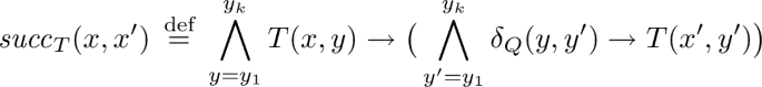
• Successors in $K_Q$ are simulated by successors in $K_P$. We first introduce the following formula $succ _T(x,x')$ to capture one-step of the simulation, that is, $x'$ follows x and for all y if T(x, y) then $x'$ simulates all successors of y (we use $\delta _Q(y, y')$ to represent that y and $y'$ states are in $\delta _{Q}$ of $K_Q$, similarly for $(x, x') \in \delta _{P}$ of $K_P$ we use $\delta _{P}(x, x'))$ :

  

  We can then define that $x_{i+1}$ follows $x_i$:

  

  (4)

  And, $x_n$ has a jump-back to a previously seen state:

  

  (5)

• Relational state predicates are fulfilled by simulation. Everything relating in the simulation fits the relational predicate, defined as a function $\textsf {\small Pred}$ of two sets of labels (we use $L_Q(y)$ to represent the set of labels on the y-encoded state in $K_Q$, similarly, $L_P(x)$ for the x-encoded state in $K_P$):

  $$\begin{aligned} \bigwedge \limits _{i=1}^n \bigwedge \limits _{j=1}^k {T}(x_i,y_j) \rightarrow \textsf {\small Pred} (L_P(x_i), L_Q(y_j)) \end{aligned}$$

  (6)

We use $\varphi _{\textsf {EA}}^{n,k}$ for the SAT formula that results of conjoining (1)-(6) for bounds n and k. If $\varphi _{\textsf {EA}}^{n,k}$ is satisfiable, then there exists $\textsf{SIM}_\textsf{EA}$ from $K_P$ to $K_Q$.

4.2 Encodings for AE-Simulation

Our goal now is to find a set of states $S_Q' \subseteq S_Q$ that is able to simulate all states in $K_P$. Therefore, as in the previous case, the state space $K_P$ corresponding to the $\forall$ quantifier will be explored exhaustively, and so $n=|K_P|$, while k is the number of states in $K_Q$, which increases in every iteration. As we have explained, this allows finding a small subset of states in $K_Q$ which suffices to simulate all states of $K_P$ (Note that here we guarantee soundness but not necessarily completeness, which will be further explained in Section 4.3).

• All states in the simulation are legal states. Again, every state guessed in the simulation is a legal state from $K_P$ or $K_Q$:

  

• $K_P$ is exhaustively explored. Every two different indices in the states of $K_P$ are different states⁴:

  

• All initial states in $K_P$ must match with some initial state in $K_Q$. Note that, contrary to the $\exists \forall$ case, here the initial state in $K_Q$ may be different for each initial state in $K_P$:

  

• For every pair in the simulation, each successor in $K_P$ must match with some successor in $K_Q$. For each $(x_i, y_j)$ in the simulation, every successor state of $x_i$ has a matching successor state of $y_j$:

  

• Relational state predicates are fulfilled. Similarly, all pairs of states in the simulation should respect the relational $\textsf {\small Pred}$:

  

We now use $\varphi _{\textsf {AE}}^{n,k}$ for the SAT formula that results of conjoining (1$^\prime$)-(5$^\prime$) for bounds n and k. If $\varphi _{\textsf {AE}}^{n,k}$ is satisfiable, then there exists $\textsf{SIM}_\textsf{AE}$ from $K_P$ to $K_Q$.

4.3 Encodings for AE-Simulation with Prophecies

The AE-simulation encoding introduced in Section 4.2 is sound but not complete (i.e., the property is satisfied, yet no simulation exists). For example, when the system for the $\forall$ quantifier is non-deterministic, the simulation is required to match immediately the successor of the $\exists$ path without inspecting the future of the $\forall$ path. In this section, we incorporate our encodings with prophecies to resolve these kind of cases, which takes us one step towards completeness. We now illustrate with the following example.

Example 1

Consider Kripke structures $K_1$ and $K_2$ from Section 1, and HyperLTL formula . It is easy to see that the two models satisfy $\varphi _2$, since mapping the sequence of states $(s_1s_2s_3)$ to $(q_1q_2q_4)$ and $(s_1s_2s_4)$ to $(q_1q_3q_5)$ guarantees that the matched paths satisfy . However, the technique in Section 4.2 cannot differentiate the occurrences of $s_2$ in the two different cases.    $\square$

To solve this, we incorporate the notion of prophecies to our setting. Prophecies have been proposed as a method to aid in the verification of hyperliveness [14] (see [7] for a systematic method to construct prophecies). For simplicity, we restrict here to prophecies expressed as safety automata. A safety prophecy over $\textsf{AP}$ is a Kripke structure $U=\langle S, S^0, \delta , \textsf{AP}, L \rangle$, such that $\textit{Traces}(U)=\textsf{AP}^\omega$. The product $K\times U$ of a Kripke structure K with a prophecy U preserves the language of K (since the language of U is universal). Recall that in the construction of the product, states $(s,u)\in (K\times U)$ that have incompatible labels are removed. The direct product can be easily processed by repeatedly removing dead states, resulting in a Kripke structure $K'$ whose language is $\textit{Traces}(K')=\textit{Traces}(K)$. Note that there may be multiple states in $K'$ that correspond to different states in K for different prophecies. The prophecy-enriched Kripke structure can be directly passed to the method in Section 4.2, so the solver can search for a $\textsf{SIM}_\textsf{AE}$ that takes the value of the prophecy into account.

Fig. 1.

Prophecy automaton for (left) and its composition with $K_1$ (right).

Example 2

Consider the prophecy automaton shown in Fig. 1 (left), where all states are initial. Note that for every state, either all its successors are labeled with a (or none are), and all successors of its successors are labeled with a (or none are). In other words, this structure encodes the prophecy . The product $K_1'$ of $K_1$ with the prophecy automaton U for is shown in Fig. 1 (right). Our method can now show that $\langle K_1',K_2\rangle \models \varphi _2$, since it can distinguish the two copies of $s_1$ (one satisfies and is mapped to $(q_1q_2q_4)$, while the other is mapped to $(q_1q_3q_5)$).    $\square$

5 Implementation and Experiments

We have implemented our algorithms using the SAT solver Z3 through its python API Z3Py  [15]. The SAT formulas introduced in Section 4 are encoded into the two scripts simEA.py and simAE.py, for finding simulation relations for the $\textsf{SIM}_\textsf{EA}$ and $\textsf{SIM}_\textsf{AE}$ cases, respectively. We evaluate our algorithms with a set of experiments, which includes all forms of quantifiers with different sizes of given models, as presented earlier in Table 1. Our simulation algorithms benefit the most in the cases of the form $\forall _\texttt {small}~\exists _\texttt {big}$. When the second model is substantially larger than the first model, $\textsf{SIM}_\textsf{AE}$ is able to prove that a $\forall \exists$ hyperproperty holds by exploring only a subset of the second model. In this section, besides $\forall _\texttt {small}~\exists _\texttt {big}$ cases, we also investigate multiple cases on each category in Table 1 to demonstrate the generality and applicability of our algorithms. All case studies are run on a MacBook Pro with Apple M1 Max chip and 64 GB of memory.

5.1 Case Studies and Empirical Evaluation

Conformance in Scenario-based Programming. In scenario-based programming, scenarios provide a big picture of the desired behaviors of a program, and are often used in the context of program synthesis or code generation. A synthesized program should obey what is specified in the given set of scenarios to be considered correct. That is, the program conforms with the scenarios. The conformance check between the scenarios and the synthesized program can be specified as a $\forall \exists$-hyperproperty:

where $\pi$ is over the scenario model and $\pi '$ is over the synthesized program. That is, for all possible runs in the scenarios, there must exists a run in the program, such that their behaviors always match.

We look into the case of synthesizing an Alternating Bit Protocol (ABP) from four given scenarios, inspired by [3]. ABP is a networking protocol that guarantees reliable message transition, when message loss or data duplication are possible. The protocol has two parties: sender and receiver, which can take three different actions: send, receive, and wait. Each action also specifies which message is currently transmitted: either a packet or acknowledgment (see [3] for more details). The correctly synthesized protocol should not only have complete functionality but also include all scenarios. That is, for every trace that appears in some scenario, there must exist a corresponding trace in the synthesized protocol. By finding $\textsf{SIM}_\textsf{AE}$ between the scenarios and the synthesized protocols, we can prove the conformance specified with $\varphi _\textsf {conf}$. Note that the scenarios are often much smaller than the actual synthesized protocol, and so this case falls in the $\forall _\texttt {small}~\exists _\texttt {big}$ category in Table 1. We consider two variations: a correct and an incorrect ABP (that cannot handle packet loss). Our algorithm successfully identifies a $\textsf{SIM}_\textsf{AE}$ that satisfies $\varphi _\textsf {conf}$ for the correct ABP, and returns UNSAT for the incorrect protocol, since the packet loss scenario cannot be simulated.

Verification of Model Translation. It is often the case that in model translation (e.g., compilation), solely reasoning about the source program does not provide guarantees about the desirable behaviors in the target executable code. Since program verification is expensive compared with repeatedly checking the target, alternative approaches such as certificate translation [4] are often preferred. Certificate translation takes inputs of a high-level program (source) with a given specification, and computes a set of verification conditions (certificates) for the low-level executable code (target) to prove that a model translation is safe. However, this technique still requires extra efforts to map the certificates to a target language, and the size of generated certificates might explode quickly (see [4] for retails). We show that our simulation algorithm can directly show the correctness of a model translation more efficiently by investigating the source and target with the same formula $\varphi _\textsf {conf}$ used for ABP. That is, the specifications from the source runs $\pi$ are always preserved in some target runs $\pi '$, which infers a correct model translation. Since translating a model into executable code implies adding extra instructions such as writing to registers, it also falls into the $\forall _\texttt {small}~\exists _\texttt {big}$ category in Table 1.

We investigate a program from [4] that performs matrix multiplication (MM). When executed, the C program is translated from high-level code (C) to low-level code RTL (Register Transfer Level), which contains extra steps to read from/write to memories. Specifications are triples of $\langle \textit{Pre}, annot , Post \rangle$, where $\textit{Pre}$, and $Post$ are assertions and $annot$ is a partial function from labels to assertions (see [4] for detailed explanations). The goal is to make sure that the translation does not violate the original verified specification. In our framework, instead of translating the certification, we find a simulation that satisfies $\varphi _\textsf {conf}$, proving that the translated code also satisfies the specification. We also investigate two variations in this case: a correct translation and an incorrect translation, and our algorithm returns SAT (i.e., finds a correct $\textsf{SIM}_\textsf{AE}$ simulation) in the former case, and returns UNSAT for the latter case.

Fig. 2.

The common branch factorization example [30].

Compiler Optimization. Secure compiler optimization aims at preserving input-output behaviors of an original implementation and a target program after applying optimization techniques, including security policies. The conformance between source and target programs guarantees that the optimizing procedure does not introduce vulnerabilities such as information leakage. Furthermore, optimization is often not uniform for the same source, because one might compile the source to multiple different targets with different optimization techniques. As a result, an efficient way to check the behavioral equivalence between the source and target provides a correctness guarantee for the compiler optimization.

Imposing optimization usually results in a smaller program. For instance, common branch factorization (CBF) finds common operations in an if-then-else structure, and moves them outside of the conditional so that such operation is only executed once. As a result, for these optimization techniques, checking the conformance of the source and target falls in the $\forall _\texttt {big}~\exists _\texttt {small}$ category. That is, given two programs, source (big) and target (small), we check the following formula:

In this case study we investigate the strategy CBF using the example in Figure 2 inspired by [30]. We consider two kinds of optimized programs for the strategy, one is the correct optimization, one containing bugs that violates the original behavior due to the optimization. For the correct version, our algorithm successfully discovered a simulation relation between the source and target, and the simulation relation returns a smaller subset of states in the second model (i.e., $|S_Q'| < |S_Q|$). For the incorrect version, we received UNSAT.

Fig. 3.

A robust path.

Robust Path Planning. In robotic planning, robustness planning (RP) refers to a path that is able to consistently complete a mission without being interfered by the uncertainty in the environment (e.g., adversaries). For instance, in the 2-D plane in Fig. 3, an agent is trying to go from the starting point (blue grid) to the goal position (green grid). The plane also contains three adversaries on the three corners other than the starting point (red-framed grids), and the adversaries move trying to catch the agent but can only move in one direction (e.g., clockwise). This is a $\exists _\texttt {small}~ \forall _\texttt {big}$ setting, since the adversaries may have several ways to cooperate and attempt to catch the agent. We formulate this planning problem as follows:

That is, there exists a robust path for the agent to safely reach the goal regardless of all the ways that the adversaries could move. We consider two scenarios, one in which there exists a way for the agent to form a robust path and one does not. Our algorithm successfully returns SAT for case which the agent can form a robust path, and returns UNSAT for which a robust path is impossible to find.

Plan Synthesis. The goal of plan synthesis (PS) is to synthesize a single comprehensive plan that can simultaneously satisfy all given small requirements has wide application in planning problems. We take the well-known toy example, wolf, goat, and cabbage⁵, as a representative case here. The problem is as follows. A farmer needs to cross a river by boat with a wolf, a goat, and a cabbage. However, the farmer can only bring one item with him onto the boat each time. In addition, the wolf would eat the goat, and the goat would eat the cabbage, if they are left unattended. The goal is to find a plan that allows the farmer to successfully cross the river with all three items safely. A plan requires the farmer to go back and forth with the boat with certain possible ways to carry different items, while all small requirements (i.e., the constraints among each item) always satisfied. In this example, the overall plan is a big model while the requirements form a much smaller automaton. Hence, it is a $\exists _\texttt {big}~ \forall _\texttt {small}$ problem that can be specified with the following formula:

Table 2. Summary of our case studies. The outcomes with simulation discovered show how our algorithms find a smaller subset for either $K_P$ or $K_Q$.

5.2 Analysis and Discussion

The summary of our empirical evaluation is presented in Table 2. For the $\forall \exists$ cases, our algorithm successfully finds a set $|S_Q'| < |S_Q|$ that satisfies the properties for the cases ABP and CBF. Note that case MM does not find a small subset, since we manually add extra paddings on the first model to align the length of both traces. We note that handling this instance without padding requires asynchornicity— a much more difficult problem, which we leave for future work. For the $\exists \forall$ cases, we are able to find a subset of $S_P$ which forms a single lasso path that can simulate all runs in $S_Q$ for all cases RP and GCW. We emphasize here that previous BMC techniques (i.e., $\textsf {\small HyperQB}$) cannot handle most of the cases in Table 2 due to the lack of loop conditions.

6 Conclusion and Future Work

We introduced efficient loop conditions for bounded model checking of fragments of HyperLTL. We proved that considering only lasso-shaped traces is equivalent to considering the entire trace set of the models, and proposed two simulation-based algorithms $\textsf{SIM}_\textsf{EA}$ and $\textsf{SIM}_\textsf{AE}$ to realize infinite reasoning with finite exploration for HyperLTL formulas. To handle non-determinism in the latter case, we combine the models with prophecy automata to provide the (local) simulations with enough information to select the right move for the inner $\exists$ path. Our algorithms are implemented using Z3py. We have evaluated the effectiveness and efficiency with successful verification results for a rich set of input cases, which previous bounded model checking approach would fail to prove.

As for future work, we are working on exploiting general prophecy automata (beyond safety) in order to achieve full generality for the $\forall \exists$ case. The second direction is to handle asynchrony between the models in our algorithm. Even though model checking asynchronous variants of HyperLTL is in general undecidable [5, 9, 25], we would like to explore semi-algorithms and fragments with decidability properties. Lastly, exploring how to handle infinite-state systems with our framework by applying abstraction techniques is also another promising future direction.

References

Martin Abadi and Leslie Lamport. The existence of refinement mappings. Theoretical Computer Science, 82:253–284, 1991.
Shreya Agrawal and Borzoo Bonakdarpour. Runtime verification of \(k\)-safety hyperproperties in HyperLTL. In Proc. of the 29th IEEE Computer Security Foundations Symp. (CSF’16), pages 239–252. IEEE, 2016.
Rajeev Alur, Milo Martin, Mukund Raghothaman, Christos Stergiou, Stavros Tripakis, and Abhishek Udupa. Synthesizing finite-state protocols from scenarios and requirements. In Proc. of the 10th Int’l Haifa Verification Conf. (HVC’14), volume 8855 of LNCS, pages 75–91. Springer, 2014.
Gilles Barthe, Benjamin Grégoire, Sylvain Heraud, César Kunz, and Anne Pacalet. Implementing a direct method for certificate translation. In Proc. of the 11th Int’l Conf. on Formal Engineering Methods (ICFEM’09), volume 5885 of LNCS, pages 541–560. Springer, 2009.
Jan Baumeister, Norine Coenen, Borzoo Bonakdarpour, Bernd Finkbeiner, and César Sánchez. A temporal logic for asynchronous hyperproperties. In Proc. of the 33rd Int’l Conf. on Computer Aided Verification (CAV’21), Part I, volume 12759 of LNCS, pages 694–717. Springer, 2021.
Saddek Bensalem, Ahmed Bouajjani, Claire Loiseaux, and Joseph Sifakis. Property preserving simulations. In Proc. of the Fourth Int’l Workshop on Computer Aided Verification (CAV’92), volume 663 of LNCS, pages 260–273. Springer, 1992.
Raven Beutner and Bernd Finkbeiner. Prophecy variables for hyperproperty verification. In Proc. of 35th IEEE Computer Security Foundations Symp. (CSF’22), pages 471–485. IEEE, 2022.
Borzoo Bonakdarpour, César Sánchez, and Gerardo Schneider. Monitoring hyperproperties by combining static analysis and runtime verification. In Proc. of the 8th Int’l Symp. on Leveraging Applications of Formal Methods, Verification and Validation (ISoLA’18), Part II, volume 11245 of LNCS, pages 8–27. Springer, 2018.
Laura Bozzelli, Adriano Peron, and César Sánchez. Asynchronous extensions of HyperLTL. In Proc. of the 36th Annual ACM/IEEE Symp. on Logic in Computer Science (LICS’21), pages 1–13. IEEE, 2021.
Noel Brett, Umair Siddique, and Borzoo Bonakdarpour. Rewriting-based runtime verification for alternation-free HyperLTL. In Proc. of the 23rd Int’l Conf. on Tools and Algorithms for the Construction and Analysis of Systems (TACAS’17), Part II, volume 10206 of LNCS, pages 77–93. Springer, 2017.
Edmund M. Clarke, Armin Biere, Richard Raimi, and Yunshan Zhu. Bounded model checking using satisfiability solving. Formal Methods in System Design (FMSD), 19(1):7–34, 2001.
Michael R. Clarkson, Bernd Finkbeiner, Masoud Koleini, Kristopher K. Micinski, Markus N. Rabe, and César Sánchez. Temporal logics for hyperproperties. In Proc. of the 3rd Int’l Conf. on Principles of Security and Trust (POST’14), volume 8414 of LNCS, pages 265–284. Springer, 2014.
Michael R. Clarkson and Fred B. Schneider. Hyperproperties. Journal of Computer Security, 18(6):1157–1210, 2010.
Norine Coenen, Bernd Finkbeiner, César Sánchez, and Leander Tentrup. Verifying hyperliveness. In Proc. of the 31st Int’l Conf. on Computer Aided Verification (CAV’19), volume 11561 of LNCS, pages 121–139. Springer, 2019.
Leonardo M. de Moura and Nikolaj Bjørner. Z3: An efficient SMT solver. In Proc. of 14th Int’l Conf. on Tools and Algorithms for the Construction and Analysis of Systems (TACAS’08), volume 4963 of LNCS, pages 337–340. Springer, 2008.
Bernd Finkbeiner, Cristopher Hahn, and Tobias Hans. MGHyper: Checking satisfiability of HyperLTL formulas beyond the \(\exists ^*\forall ^*\) fragment. In Proc. of the 16th Int’l Symp. on Automated Technology for Verification and Analysis (ATVA’18), volume 11138 of LNCS, pages 521–527. Springer, 2018.
Bernd Finkbeiner, Cristopher Hahn, and Marvin Stenger. EAHyper: Satisfiability, implication, and equivalence checking of hyperproperties. In Proc. of the 29th Int’l Conf. on Computer Aided Verification (CAV’17), Part II, volume 10427 of LNCS, pages 564–570. Springer, 2017.
Bernd Finkbeiner, Cristopher Hahn, Marvin Stenger, and Leander Tentrup. RVHyper: A runtime verification tool for temporal hyperproperties. In Proc. of the 24th Int’l Conf. on Tools and Algorithms for the Construction and Analysis of Systems (TACAS’18), Part II, volume 10806 of LNCS, pages 194–200. Springer, 2018.
Bernd Finkbeiner, Cristopher Hahn, Marvin Stenger, and Leander Tentrup. Monitoring hyperproperties. Formal Methods in System Design (FMSD), 54(3):336–363, 2019.
Bernd Finkbeiner, Cristopher Hahn, and Hazem Torfah. Model checking quantitative hyperproperties. In Proc. of the 30th Int’l Conf. on Computer Aided Verification (CAV’18), Part I, volume 10981 of LNCS, pages 144–163. Springer, 2018.
Bernd Finkbeiner, Christian Müller, Helmut Seidl, and Eugene Zalinescu. Verifying security policies in multi-agent workflows with loops. In Proc. of the 15th ACM Conf. on Computer and Communications Security (CCS’17), pages 633–645. ACM, 2017.
Bernd Finkbeiner, Markus N. Rabe, and César Sánchez. Algorithms for model checking HyperLTL and HyperCTL*. In Proc. of the 27th Int’l Conf. on Computer Aided Verification (CAV’15), Part I, volume 9206 of LNCS, pages 30–48. Springer, 2015.
Ohad Goudsmid, Orna Grumberg, and Sarai Sheinvald. Compositional model checking for multi-properties. In Proc. of the 22nd Int’l Conf. on Verification, Model Checking, and Abstract Interpretation (VMCAI’21), volume 12597 of LNCS, pages 55–80. Springer, 2021.
Orna Grumberg and David E. Long. Model checking and modular verification. ACM Transactions on Programming Languages and Systems (TOPLAS), 16(3):843–871, 1994.
Jens Oliver Gutsfeld, Markus Müller-Olm, and Christoph Ohrem. Automata and fixpoints for asynchronous hyperproperties. Proc. ACM Program. Lang., 5:1–29, 2021.
Cristopher Hahn, Marvin Stenger, and Leander Tentrup. Constraint-based monitoring of hyperproperties. In Proc. of the 25th Int’l Conf. on Tools and Algorithms for the Construction and Analysis of Systems (TACAS’19), volume 11428 of LNCS, pages 115–131. Springer, 2019.
Tzu-Han Hsu, César Sánchez, and Borzoo Bonakdarpour. Bounded model checking for hyperproperties. In Proc. of the 27th Int’l Conf on Tools and Algorithms for the Construction and Analysis of Systems (TACAS’21). Part I, volume 12651 of LNCS, pages 94–112. Springer, 2021.
Tzu-Han Hsu, César Sánchez, Sarai Sheinvald, and Borzoo Bonakdarpour. Efficient loop conditions for bounded model checking hyperproperties. CoRR, abs/2301.06209, 2023.
Orna Kupferman and Moshe Y. Vardi. Model checking of safety properties. In Proc. of the 11th Int’l Conf. on Computer Aided Verification (CAV’99), volume 1633 of LNCS, pages 172–183. Springer, 1999.
Kedar S. Namjoshi and Lucas M. Tabajara. Witnessing secure compilation. In Proc. of the 21st Int’l Conf. on Verification, Model Checking, and Abstract Interpretation (VMCAI’20), volume 11990 of LNCS, pages 1–22. Springer, 2020.
Amir Pnueli. The temporal logic of programs. In Proc. of the 18th Symp. on Foundations of Computer Science (FOCS’77), pages 46–57. IEEE, 1977.
Amir Pnueli. Applications of temporal logic to the specification and verification of reactive systems: A survey of current trends. In Proc. of Current Trends in Concurrency, Overviews and Tutorials, volume 224 of LNCS, pages 510–584. Springer, 1985.
Sandro Stucki, César Sánchez, Gerardo Schneider, and Borzoo Bonakdarpour. Graybox monitoring of hyperproperties. In Proc. of the 23rd Int’l Symp. on Formal Methods (FM’19), volume 11800 of LNCS, pages 406–424. Springer, 2019.
Moshe Y. Vardi and Pierre Wolper. Automata theoretic techniques for modal logic of programs. Journal of Computer and System Sciences, 32(2):183–221, 1986.
Author information
Authors and Affiliations
Corresponding author
Editor information
Editors and Affiliations
Rights and permissions
Open Access This chapter is licensed under the terms of the Creative Commons Attribution 4.0 International License (http://creativecommons.org/licenses/by/4.0/), which permits use, sharing, adaptation, distribution and reproduction in any medium or format, as long as you give appropriate credit to the original author(s) and the source, provide a link to the Creative Commons license and indicate if changes were made.
The images or other third party material in this chapter are included in the chapter's Creative Commons license, unless indicated otherwise in a credit line to the material. If material is not included in the chapter's Creative Commons license and your intended use is not permitted by statutory regulation or exceeds the permitted use, you will need to obtain permission directly from the copyright holder.
Copyright information
© 2023 The Author(s)
About this paper
Cite this paper
Hsu, TH., Sánchez, C., Sheinvald, S., Bonakdarpour, B. (2023). Efficient Loop Conditions for Bounded Model Checking Hyperproperties. In: Sankaranarayanan, S., Sharygina, N. (eds) Tools and Algorithms for the Construction and Analysis of Systems. TACAS 2023. Lecture Notes in Computer Science, vol 13993. Springer, Cham. https://doi.org/10.1007/978-3-031-30823-9_4
Download citation
DOI: https://doi.org/10.1007/978-3-031-30823-9_4
Published:
Publisher Name: Springer, Cham
Print ISBN: 978-3-031-30822-2
Online ISBN: 978-3-031-30823-9
eBook Packages: Computer ScienceComputer Science (R0)