Construction of Suitable Covers and Proof of the Main Theorem

Abstract

In this chapter, we set up some theory concerning the action of isometries on fundamental groups and first homology groups. More specifically, we show that the action of a finite group of isometries on the first homology group of a manifold corresponds to conjugation by a lift to the orbifold fundamental group of the quotient. This result is then used to give a necessary and sufficient condition for realising a certain wreath product by a Galois cover (by an explicit construction of the corresponding subgroup of the fundamental group)—a problem similar to the algebraic problem of inverse Galois theory. The required condition, called (∗), is a representation-theoretic property of the action on homology. Using the representation theoretical results from the previous chapter, this allows us to finish the proof of the main theorem of the text, describing covering equivalence of manifolds through spectra of twisted Laplacians.

In this chapter, we set up some theory concerning the action of isometries on fundamental groups and first homology groups. More specifically, we show that the action of a finite group of isometries on the first homology group of a manifold corresponds to conjugation by a lift to the orbifold fundamental group of the quotient. This result is then used to give a necessary and sufficient condition for realising a certain wreath product by a Galois cover (by an explicit construction of the corresponding subgroup of the fundamental group)—a problem similar to the algebraic problem of inverse Galois theory. The required condition, called (∗), is a representation-theoretic property of the action on homology. Using the representation theoretical results from the previous chapter, this allows us to finish the proof of the main theorem of the text, describing covering equivalence of manifolds through spectra of twisted Laplacians.

1 Fundamental Group and First Homology

We first fix some notations and constructions. Let M denote a connected closed oriented smooth Riemannian manifold. Fixing a point x ∈ M, the universal covering $\widetilde M$ is described as the set of homotopy classes [w] of paths w : [0, 1] → M with w(0) = x. This provides a projection map

$$\displaystyle \begin{aligned} \Pi: (\widetilde M,\widetilde x) \to (M,x),\ \Pi([w]) = w(1), \end{aligned}$$

where $\widetilde x \in \widetilde M$ represents the homotopy class of the constant path at x. If we equip $\widetilde M$ with the pull-back of the Riemannian metric on M then the group Γ acts isometrically by deck transformations on $\widetilde M$, and M is identified with the quotient $\Gamma \backslash \widetilde M$.

Let ∗ denotes path-concatenation read from left to right, that is, [a] ∗ [b] is the homotopy class of the path obtained by first traversing a and then b. Letting $\widetilde x$ denote the constant path at x, we have an identification

$$\displaystyle \begin{aligned} \Phi_{\widetilde x}: \Gamma \to \pi_1(M,x) \end{aligned}$$

via the map $\Phi _{\widetilde x}(\gamma ) = \gamma (\widetilde x)$, with $\gamma (\widetilde x)$ representing a homotopy class of a closed loop starting and ending at x. More generally, any homotopy class of a path [w] in $\widetilde M$ induces a map Φ_[w] :  Γ → π ₁(M, w(1)) via

$$\displaystyle \begin{aligned} \Phi_{[w]}(\gamma) = [w^{-1}] * \Phi_{\widetilde x}(\gamma) * [w]. \end{aligned} $$

(6.1)

We denote the first homology group of M (with integer coefficients) by $\operatorname {H}_1(M) = \operatorname {H}_1(M,\mathbf {Z})$. The universal coefficient theorem for homology [48, §3.A] implies that for any field K, we have an isomorphism

$$\displaystyle \begin{aligned} \operatorname{H}_1(M,K) = \operatorname{H}_1(M) \otimes_{\mathbf{Z}} K. \end{aligned}$$

Also, since M is a connected manifold, it is path-connected, so that we have a Hurewicz homomorphism inducing an identification

$$\displaystyle \begin{aligned} \operatorname{H}_1(M) = \pi_1(M,x)^{\operatorname{ab}} \cong \Gamma^{\operatorname{ab}}. \end{aligned}$$

The map is given by considering a (homotopy class of a) loop as a concatenation of oriented 1-cells and mapping it to the (homology class of the) signed sum of those cells.

Composing the maps, we have a homomorphism $\Psi _0: \Gamma \to \operatorname {H}_1(M,{\mathbf {F}}_\ell )$ given as the composition of Φ_[w] with the abelianisation map and the Hurewicz isomorphism, followed by reduction modulo ℓ:

(6.2)

Since by (6.1) the homotopy classes of loops Φ_[w] for different w are freely homotopic, the composed map Ψ₀ is independent of the choice of w, as notation indicates. The standard choice is $w=\widetilde x$, but we will naturally encounter others.

2 First Homology and Galois Covers

Suppose now that G is a finite group of isometries acting on M, and let q: M → M ₀ denote the orbifold quotient, with Γ₀ the covering group of $\Pi _0 \colon \widetilde M \rightarrow M_0$. Let Γ be the normal subgroup of Γ₀ corresponding to $\Pi \colon \widetilde M \rightarrow M$, so that there is a short exact sequence of groups

$$\displaystyle \begin{aligned} 1 \rightarrow \Gamma \rightarrow \Gamma_0 \xrightarrow{F} G \rightarrow 1 \end{aligned} $$

(6.3)

giving an isomorphism G≅ Γ₀∕ Γ. The setup is summarised in diagram (6.4).

(6.4)

Definition 6.2.1

For γ ₀ ∈ Γ₀, let $\operatorname {conj}_{\gamma _0}: \Gamma \to \Gamma$ be conjugation by γ ₀, that is

$$\displaystyle \begin{aligned} \operatorname{conj}_{\gamma_0}(\gamma) = \gamma_0 \gamma \gamma_0^{-1}. \end{aligned}$$

Remark 6.2.2

If g ∈ G≅ Γ₀∕ Γ satisfies g = γ ₀ Γ, this represents the usual map

$$\displaystyle \begin{aligned} G \rightarrow \mathrm{Out}(\Gamma) \colon g \mapsto \operatorname{conj}_{\gamma_0} \end{aligned}$$

induced by the exact sequence (6.3), where Out( Γ) = Aut( Γ)∕Inn( Γ) is the quotient of the group of automorphisms of Γ by the group $\mathrm {Inn}(\Gamma ) = \{ \operatorname {conj}_\gamma \colon \gamma \in \Gamma \}$ of inner automorphisms.

In this setup, the action of the isometry g on M corresponds to the action of $\operatorname {conj}_{\gamma _0^{-1}}$ on Γ, so that there is a commuting diagram

(6.5)

The action of G on M by isometries induces a linear action of G on $\operatorname {H}_1(M,{\mathbf {F}}_\ell )$, providing an F _ℓ[G]-module structure on this homology group. The following lemma describes the relation between this action and the above outer conjugation on Γ: they commute by the Hurewicz map. The argument is similar to the one used in the proof of Hopf’s formula [21, (5.3)].

Lemma 6.2.3

Let γ ₀ ∈ Γ ₀ and g ∈ G≅ Γ ₀∕ Γ such that g = γ ₀  Γ. Then the following diagram commutes:

(6.6)

where Ψ ₀ is as in (6.2) and the bottom line indicates the action of g ∈ G on the first homology group.

Proof

The vertical maps are given by picking a base point x ∈ M, considering γ ∈ Γ as a homotopy class of a closed loop in M based at x via $\Phi _{\widetilde x}$, rewriting γ as a concatenation of oriented 1-cells, and mapping these to the corresponding sum of 1-cells in homology. The crucial observation that makes the proof work is that we can decompose into 1-cells, not just 1-cycles, and the image is independent of the choice of base point. In this way, the closed loop corresponding to $\operatorname {conj}_{\gamma _0}(\gamma )$ decomposes as a (left-to-right) concatenation of the 1-cells

$$\displaystyle \begin{aligned} (\gamma_0: x \rightarrow gx) \ast ( g \cdot \gamma: gx \rightarrow gx) \ast (\gamma_0^{-1}: gx \rightarrow x), \end{aligned}$$

that is mapped by Ψ₀ to the sum of homology classes [γ ₀] + g ⋅ [γ] − [γ ₀] = g ⋅ [γ], proving the commutativity of the diagram. □

Remark 6.2.4

In fact, there is a larger commutative diagram:

(6.7)

The detailed proof goes as follows: we have argued before that both vertical maps (from top to bottom) on the left and right hand side of (6.7) agree and are equal to Ψ₀. Naturality of the Hurewicz isomorphism guarantees commutativity of the lower square in (6.7) and it therefore suffices to prove commutativity of the upper square in (6.7).

Elements g ∈ G are isometries g : M → M and the groups Γ₀ and Γ acting by isometries on $\widetilde M$ can be described via deck transformations as follows

$$\displaystyle \begin{aligned} \$ \Gamma := \{ I: \widetilde M \to \widetilde M\, \text{isometry} \mid F(I([w])) = F([w])\, \forall\, [w] \in \widetilde M \}, \\ \$ \Gamma_0 := \{ I: \widetilde M \to \widetilde M\, \text{isometry} \mid \exists\, g \in G: F(I([w]) = g F([w])\, \forall\, [w] \in \widetilde M \}. {} \end{aligned} $$

(6.8)

In this description, the map F :  Γ → G from (6.3) is given by mapping I ∈ Γ₀ to the (uniquely determined) corresponding element g ∈ G in (6.8).

Let π ₁(M, x, y) denote the set of homotopy classes of paths in M from x to y. We identify the elements in Γ₀ with homotopy classes of paths starting at x via the following bijective map:

$$\displaystyle \begin{aligned} \begin{array}{rcl} \pi_1(M,x,gx) \$ \to\$\displaystyle F^{-1}(g) \subset \Gamma_0, {} \\ {[a]} \$ \mapsto\$\displaystyle I_a \colon [w] \mapsto [a] * [gw] . \end{array} \end{aligned} $$

(6.9)

It can be easily checked that $I_a^{-1}([w]) = [g^{-1}a^{-1}] * [g^{-1}w].$ To prove commutativity of the upper square of diagram (6.7), we go around the square both ways.

• Computing $\Phi _{\gamma _0 \widetilde x}(\operatorname {conj}_{\gamma _0}(\gamma ))$. We first describe the conjugation action in terms of concatenation. Using (6.9), we identify γ ₀ with a map $I_a: \widetilde M \to \widetilde M$ for a path a satisfying a(0) = x and a(1) = gx. Similarly, we identify γ with a map $I_c: \widetilde M \to \widetilde M$ for a path c satisfying c(0) = c(1) = x. For any $\widetilde y =[w] \in \widetilde M$ with a path w in M starting at w(0) = x, we have

  $$\displaystyle \begin{aligned} \operatorname{conj}_{\gamma_0}(\gamma)(\widetilde y) = I_a(I_c(I_a^{-1}([w]))) = [a] * [gc] * [a^{-1}] * [w] \end{aligned}$$

  and, in particular,

  $$\displaystyle \begin{aligned} \operatorname{conj}_{\gamma_0}(\gamma)(\widetilde x) = [a] * [gc] * [a^{-1}]. \end{aligned}$$

  Now we evaluate $\Phi _{\gamma _0 \widetilde x}(\operatorname {conj}_{\gamma _0}(\gamma ))$. We first note that

  $$\displaystyle \begin{aligned} \gamma_0 \widetilde x = I_a(\widetilde x) = [a] * (g \widetilde x) = [a], \end{aligned}$$

  since $g \widetilde x$ is the homotopy class of the constant path at gx in M. This implies

  $$\displaystyle \begin{aligned} \Phi_{\gamma_0 \widetilde x}(\operatorname{conj}_{\gamma_0}(\gamma)) \$ = [a^{-1}] * \Phi_{\widetilde x}(\operatorname{conj}_{\gamma_0}(\gamma)) * [a] \\ \$= [a^{-1}] * \operatorname{conj}_{\gamma_0}(\gamma)(\widetilde x) * [a] \\ \$= [gc]. \end{aligned} $$

• Computing $g \cdot \Phi _{\widetilde x}(\gamma )$. We have $g \cdot \Phi _{\widetilde x}(\gamma ) = g \cdot \gamma (\widetilde x) = g \cdot I_c(\widetilde x) = g \cdot ([c] * \widetilde x) = [g c].$

Since the results of the two computations agree, the proof is finished.

3 Realisability of the Wreath Product

The following result gives an exact topological criterion for realisation of the wreath product, in terms of the F _ℓ[G]-module structure of $\operatorname {H}_1(M,{\mathbf {F}}_\ell )$.

Proposition 6.3.1

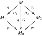
Suppose that we have a diagram of Riemannian coverings

(6.10)

with M ₀ a developable orbifold and M, M ₁ manifolds. Fix a prime ℓ, set C = Z∕ℓ Z and consider the wreath products $\widetilde G$ and $\widetilde H_1$ as in Definition 5.2.1 (with H = H ₁ ). Let {g ₁ H ₁ = H ₁, g ₂ H ₁, …, g _n H ₁} denote the cosets in G∕H ₁ . For any g ∈ G, define the permutation i↦g(i) on {1, …, n} and the element h _g,i ∈ H ₁ via gg _i = g _g(i) h _g,i.

Define the F _ℓ[G]-module $\mathscr N$ as $\mathscr N:=(\operatorname {Ind}_{H_1}^G \mathbf {1}) \otimes _{\mathbf {Z}} {\mathbf {F}}_\ell$ (cf. Remark 5.2.2 ). Then the diagram (6.10) can be extended to a diagram of the form (5.6) if and only if $\mathscr N$ is a F _ℓ[G]-quotient module of $\operatorname {H}_1(M,{\mathbf {F}}_\ell )$.

Proof

We fix the following for the duration of the proof.

• Set $\mathscr M:=\operatorname {H}_1(M,{\mathbf {F}}_\ell )$.

• Let $e_i = (0,\dots ,0,1,0,\dots ,0) \in C^n \cong {\mathbf {F}}_\ell ^n$ denote the standard “basis vectors”.

• As in Remark 5.2.2, we identify $\mathscr N \cong C^n \cong {\mathbf {F}}_\ell ^n$ as F _ℓ[G]-modules, where the action of G on C ⁿ given by the permutation representation of the cosets implemented by the map (5.1) used to define the wreath product, i.e., $\Phi \colon G \rightarrow \operatorname {Aut}(C^n) \colon g \mapsto (e_i \mapsto e_{g(i)})$.

• $\widetilde M$ is the universal covering of M, $M_0 = \Gamma _0 \backslash \widetilde M$, $M_1 = \Gamma _1 \backslash \widetilde M$ and $M = \Gamma \backslash \widetilde M$.

• F is the map from (6.3).

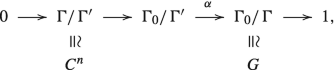
In one direction, assume the extended cover exists, corresponding to a quotient of Γ. Now M′→ M is a Galois cover with group the elementary abelian ℓ-group C ⁿ. Using the universal property of abelianisation, the corresponding map Γ → C ⁿ, whose kernel we denote by Γ′, factors through to a map of F _ℓ-vector spaces

$$\displaystyle \begin{aligned} \varphi \colon \mathscr M \twoheadrightarrow C^n \cong \mathscr N. \end{aligned}$$

We claim that this is a map of F _ℓ[G]-modules. For each g ∈ G consider the corresponding element $\widetilde g=(0,g) \in \widetilde G$. Let γ ₀ ∈ Γ₀ denote any lift of $\widetilde g$ (i.e., $\widetilde g = \gamma _0 \Gamma ' \in \widetilde G=\Gamma _0/\Gamma '$). By Lemma 6.2.3 applied to both M′ and M, $\widetilde g$ acts on Γ′ and g acts on Γ as $\operatorname {conj}_{\gamma _0}$. Hence $\widetilde g$ acts on Γ∕ Γ′ = C ⁿ as conjugation by $\gamma _0 \Gamma ' = \widetilde g$. Now in the semidirect product $\widetilde G$, the action of $\widetilde g$ on c ∈ C ⁿ is given by conjugation $c \mapsto \widetilde g c \widetilde g^{-1}$, which corresponds to the action of G on C ⁿ via Φ, i.e., gives the F _ℓ[G]-module structure $\mathscr N$ to C ⁿ. Therefore, φ(gm) = gφ(m), as desired.

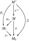
Conversely, suppose there exists a map $\varphi \colon \mathscr M \twoheadrightarrow \mathscr N$ of F _ℓ[G]-modules. Precomposing with Ψ₀ as in (6.2), we get a map Ψ:  Γ → C ⁿ, and we set

$$\displaystyle \begin{aligned} \Gamma' := \ker \Psi \vartriangleleft \Gamma\mbox{ and } M':=\Gamma' \backslash M.\end{aligned} $$

(6.11)

With this map we can also extend the commutative diagram (6.6) as follows:

(6.12)

where the commutativity of the bottom square is guaranteed precisely by our assumption that φ is a map of F _ℓ[G]-modules.

It remains to verify that the manifold M′ fits into a diagram (5.6). For this, we need to prove that Γ′ is normal in Γ₀ (hence also normal in Γ and Γ₁) such that there are induced group isomorphisms $\Gamma _0 / \Gamma ' \cong \widetilde G$, $\Gamma _1 / \Gamma ' \cong \widetilde H_1$ and Γ∕ Γ′≅C ⁿ, where $\widetilde G = C^n \rtimes G$ is the wreath product introduced in Definition 5.2.1 (with H = H ₁). For this, we show that the group Γ′ has the following properties (i)–(v).

• (i) Γ′ is normal in Γ₀; indeed, commutativity of diagram (6.12) implies that if γ ₀ ∈ Γ₀ with F(γ ₀) = g and Ψ(γ′) = 0 (i.e., γ′∈ Γ′), then $\Psi (\operatorname {conj}_{\gamma _0}(\gamma '))=\Phi (g)\Psi (\gamma ')=0$ (i.e., $\gamma _0 \gamma ' \gamma _0^{-1} \in \Gamma ')$.

Fix a set-theoretic section $G \rightarrow \Gamma _0 \colon g \mapsto \overline g$ of the map F, i.e., for any g ∈ G fix any $\overline g \in \Gamma _0$ such that $F(\overline g)=g$. Fix an element c ∈ Γ with Ψ(c) = e ₁ (which exists since Ψ is surjective), and for i = 1, …, n, let $c_i := \overline g_i c \overline g_i^{-1} \in \Gamma _0.$ Notice that

$$\displaystyle \begin{aligned} \Psi(c_i) = \Phi(g_i)e_1 = e_i. \end{aligned} $$

(6.13)

Then we have the following properties:

• (ii) c _i c _j Γ′ = c _j c _i Γ′ for all 1 ≤ i, j ≤ n. This follows since Γ∕ Γ′≅C ⁿ is commutative.

• (iii) The cosets of Γ′ in Γ₀ are represented by $\overline g c_1^{k_1} \cdots c_n^{k_n} \Gamma '$ with g ∈ G and 0 ≤ k ₁, …, k _n < ℓ. From (6.13) we see that $c_1^{k_1} \cdots c_n^{k_n} \Gamma '$ are the cosets of Γ∕ Γ′, and this combines with G≅ Γ₀∕ Γ.

• (iv) $\overline g c_i \Gamma ' = c_{g(i)}\overline g \Gamma '$ for all g ∈ G. Indeed,

  $$\displaystyle \begin{aligned} \Psi(\overline g c_i \overline g^{-1}) \stackrel{(6.12)}{=} \Phi(g)\Psi(c_i) \stackrel{(6.13)}{=} \Phi(g)(e_i) \stackrel{(5.1)}{=} e_{g(i)} \stackrel{(6.13)}{=} \Psi(c_{g(i)}). \end{aligned}$$

  It follows that $\overline g c_i \overline g^{-1} \Gamma ' = c_{g(i)} \Gamma '$ and, since Γ′ is normal in Γ₀, we can interchange left and right cosets and multiply on the right with $\overline g$ to find the result.

By (iii) and (iv), the cosets of Γ₀∕ Γ′ are given by $\overline g c_1^{k_1} \cdots c_n^{k_n} \Gamma ' = c_{g(1)}^{k_1} \cdots c_{g(n)}^{k_n} \overline g \Gamma '$ with g ∈ G and 0 ≤ k ₁, …, k _n < ℓ. Define $\widehat \Psi : \Gamma _0 \to \widetilde G = C^n \rtimes G$ by

$$\displaystyle \begin{aligned} \widehat \Psi(c_1^{k_1} \cdots c_n^{k_n} \overline g \Gamma') = (k_1,\dots,k_n,g). \end{aligned}$$

• (v) Using the commutativity property in (ii), we have for $k_i,k_j^{\prime } \in \{0,1,\dots ,\ell -1\}$, and g, g′∈ G,

  $$\displaystyle \begin{aligned} \left( c_1^{k_1} \cdots c_n^{k_n} \overline g \Gamma^{\prime} \right) \left( c_1^{k_1^{\prime}} \cdots c_n^{k_n^{\prime}} \overline g^{\prime} \Gamma^{\prime} \right) = \left( c_1^{k_1} \cdots c_n^{k_n} c_{g(1)}^{k_1^{\prime}} \cdots c_{g(n)}^{k_n^{\prime}} \right) (\overline g \cdot \overline g^{\prime}) \Gamma^{\prime}, \end{aligned}$$

  which follows immediately from (i) and (iv).

• (vi) Via a modification of the section G → Γ₀, $g \mapsto \overline g$, the map $\widehat \Psi$ becomes a surjective group homomorphism with kernel Γ′. This follows immediately from (v) if we can choose the section in such a way that $(\overline g \cdot \overline g') \Gamma ' = \overline {g\cdot g'} \Gamma '$. Consider the short exact sequence

  

  (6.14)

  with the canonical maps. Note that Γ∕ Γ′≅C ⁿ is a G-module via the action

  $$\displaystyle \begin{aligned} g \cdot \left( c_1^{k_1} \cdot c_n^{k_n} \Gamma' \right) = c_{g(1)}^{k_1} \cdot c_{g(n)}^{k_n} \Gamma'. \end{aligned}$$

  Since the order of G is coprime to that of C ⁿ, we have the vanishing of group cohomology:

  $$\displaystyle \begin{aligned} \operatorname{H}^1(G,\Gamma/\Gamma') = \operatorname{H}^2(G,\Gamma/\Gamma') = 0 \end{aligned}$$

  [21, IV 2.3, 3.12, 3.13] and hence (6.14) splits; let ȷ denote a group homomorphism ȷ : G → Γ₀∕ Γ′ such that α ∘ ȷ = id_G. Redefine the section G → Γ₀ in such a way that $\overline g \Gamma ' = \jmath (g)$. Then we have

  $$\displaystyle \begin{aligned} (\overline g \cdot \overline g') \Gamma' = \overline g \Gamma' \cdot \overline g' \Gamma' = \jmath(g) \cdot \jmath(g') = \jmath(gg') = \overline{g\cdot g'} \Gamma' \end{aligned}$$

  and $\widehat \Psi : \Gamma _0 \to \widetilde G$ is a surjective group homomorphism with kernel Γ′.

It follows that $\widehat \Psi$ induces an isomorphism $\Gamma _0/\Gamma ' \cong \widetilde G$. We have already seen the isomorphism Γ∕ Γ′≅C ⁿ in the proof of (ii). To show that $\Gamma _1/\Gamma ' \cong \widetilde H_1$ and finish the proof, note that $c_1^{k_1} \cdots c_n^{k_n} \overline h \Gamma '$ with k _i ∈{0, …, ℓ − 1} and h ∈ H ₁ are the cosets of Γ₁∕ Γ′ and that the quotient Γ₁∕ Γ′ is isomorphic to the subgroup $\widetilde H_1$ of $\widetilde G$ under the restriction of the isomorphism induced by $\widehat \Psi$. □

4 Main Result

We can now prove the main result.

Theorem 6.4.1

Suppose M ₁ and M ₂ are two connected closed oriented smooth Riemannian manifolds such that there is a diagram

of finite covers of a developable Riemannian orbifold M ₀ , as in (1.1) . Then

• (i) The diagram (1.1) may be extended to a diagram of finite coverings

  

  as in (1.2) , where M is a connected closed smooth Riemannian manifold M with three Galois covers

  $$\displaystyle \begin{aligned} q_1 \colon M \twoheadrightarrow M_1:=H_1 \backslash M,\\ q_2 \colon M \twoheadrightarrow M_2:=H_2 \backslash M\\ q \colon M \twoheadrightarrow M_0:=G\backslash M. \end{aligned} $$

Suppose furthermore that there exists a prime number ℓ ≥ 3 such that

$$\displaystyle \begin{aligned} (\ast) \ (\operatorname{Ind}_{H_1}^G \mathbf{1}) \otimes_{\mathbf{Z}} {\mathbf{F}}_\ell \ \mathit{is \ an} \ {\mathbf{F}}_\ell[G]\mathit{-quotient \ module \ of} \ \operatorname{H}_1(M,{\mathbf{F}}_\ell). \end{aligned}$$

Then

• (ii) There exists a diagram of Riemannian coverings

  

  as in (5.6) , where C = Z∕ℓ Z, $\widetilde G = C^n \rtimes G$ is the wreath product where G permutes the copies of C in the same way as it permutes the cosets of H ₁ in G, and $\widetilde H_i = C^n \rtimes H_i$ are subgroups of $\widetilde G$ corresponding to the groups H _i , i = 1, 2.

• (iii) Consider the linear character

  $$\displaystyle \begin{aligned} \Xi \colon \widetilde H_1 \rightarrow {\mathbf{C}}^* \colon (k_1,\dots,k_n,h_1) \rightarrow e^{2 \pi i k_1}/\ell \end{aligned}$$

  with (k ₁, …, k _n) ∈ C ⁿ and h ₁ ∈ H ₁ . Then the manifolds M ₁ and M ₂ are equivalent Riemannian covers of M ₀ if and only if there exists a linear character $\chi \colon \widetilde H_2 \rightarrow \operatorname {U}(1, \mathbf {C})$ such that the multiplicity of zero in the following two pairs of spectra of twisted Laplacians on M ₁ and M ₂ coincide:

  $$\displaystyle \begin{aligned} \sigma_{M_1}(\overline \Xi \otimes \operatorname{Res}_{\widetilde H_1}^{\widetilde G} \operatorname{Ind}_{\widetilde H_1}^{\widetilde G} \Xi) \mathit{\mbox{ and }} \sigma_{M_2}(\overline \chi \otimes \operatorname{Res}_{\widetilde H_2}^{\widetilde G} \operatorname{Ind}_{\widetilde H_1}^{\widetilde G} \Xi) \end{aligned}$$

  and

  $$\displaystyle \begin{aligned} \sigma_{M_1}(\overline \Xi \otimes \operatorname{Res}_{\widetilde H_1}^{\widetilde G} \operatorname{Ind}_{\widetilde H_2}^{\widetilde G} \chi) \mathit{\mbox{ and }} \sigma_{M_2}(\overline \chi \otimes \operatorname{Res}_{\widetilde H_2}^{\widetilde G} \operatorname{Ind}_{\widetilde H_2}^{\widetilde G} \chi). \end{aligned}$$

  There are $\ell |H_2^{\operatorname {ab}}|$ linear characters χ on $\widetilde H_2$ , and the dimension of the representations involved is the index [G : H ₂].

Proof

Part (i) holds by Proposition 2.4.1. Part (ii) is shown in Proposition 6.3.1. Then (iii) holds by Corollary 5.3.1 and Proposition 5.3.2, using that the character Ξ given in (iii), is the one constructed in the proof of Proposition 5.2.3 (cf. formula (5.2)), and is $\widetilde G$-solitary on $\widetilde H_1$. □

Remark 6.4.2

Using Proposition 3.10.1, the condition on the multiplicity of zero in the spectrum of the indicated twisted Laplacians in Theorem 6.4.1 may be replaced by an equality of their spectral zeta functions, if we assume in addition that M ₁ and M ₂ are isospectral, i.e., $\zeta _{M_1, \Delta _{M_1}} = \zeta _{M_2, \Delta _{M_2}}$.

Condition (∗) in the main theorem can be varied, as we will see in the next two chapters. This will also produce a geometric realisation of M′ and a set of examples where the condition holds.

Project

Describe a theory of (homological) conditions for the realisability of general extensions of finite groups 1 → A → G → H → 1 with abelian kernel A, extending a given H-covering; note that a theory of abelian coverings of a given manifold—the case where H is trivial—is encoded almost tautologically in the first homology group, since it is the abelinization of the fundamental group.

References

Kenneth S. Brown, Cohomology of groups, Graduate Texts in Mathematics, vol. 87, Springer-Verlag, New York-Berlin, 1982.
Allen Hatcher, Algebraic topology, Cambridge University Press, Cambridge, 2002, available from http://pi.math.cornell.edu/~hatcher/AT/ATpage.html.
Author information
Authors and Affiliations
Rights and permissions
Open Access This chapter is licensed under the terms of the Creative Commons Attribution 4.0 International License (http://creativecommons.org/licenses/by/4.0/), which permits use, sharing, adaptation, distribution and reproduction in any medium or format, as long as you give appropriate credit to the original author(s) and the source, provide a link to the Creative Commons license and indicate if changes were made.
The images or other third party material in this chapter are included in the chapter's Creative Commons license, unless indicated otherwise in a credit line to the material. If material is not included in the chapter's Creative Commons license and your intended use is not permitted by statutory regulation or exceeds the permitted use, you will need to obtain permission directly from the copyright holder.
Copyright information
© 2023 The Author(s)
About this chapter
Cite this chapter
Cornelissen, G., Peyerimhoff, N. (2023). Construction of Suitable Covers and Proof of the Main Theorem. In: Twisted Isospectrality, Homological Wideness, and Isometry . SpringerBriefs in Mathematics. Springer, Cham. https://doi.org/10.1007/978-3-031-27704-7_6
Download citation
DOI: https://doi.org/10.1007/978-3-031-27704-7_6
Published:
Publisher Name: Springer, Cham
Print ISBN: 978-3-031-27703-0
Online ISBN: 978-3-031-27704-7
eBook Packages: Mathematics and StatisticsMathematics and Statistics (R0)