Improving Pre-trained Language Models

Abstract

This chapter describes a number of different approaches to improve the performance of Pre-trained Language Models (PLMs), i.e. variants of BERT, autoregressive language models similar to GPT, and sequence-to-sequence models like Transformers. First we may modify the pre-training tasks to learn as much as possible about the syntax and semantics of language. Then we can extend the length of the input sequence to be able to process longer inputs. Multilingual models are simultaneously trained with text in different languages. Most important is the inclusion of further knowledge into the PLM to produce better predictions. It turns out that by increasing the number of parameters, the size of the training data and the computing effort the performance of the models can always be increased. There are a number of different fine-tuning strategies which allow the model to be adapted to special tasks. In addition, models may be instructed by few-shot prompts to solve specific tasks. This is especially rewarding for larger PLMs, which therefore are called Foundation Models.

This chapter describes a number of different approaches to improve the performance of Pre-trained Language Models (PLMs), i.e. variants of BERT, autoregressive language models similar to GPT, and sequence-to-sequence models like Transformers. When these models have a large number of parameters, they can be instructed by input prompts to solve new tasks and are called Foundation Models.

• Modification of the pre-training tasks. During pre-training with a large corpus the PLM should learn as much as possible about the syntax and semantics of language. By adapting and enhancing the pre-training objectives the performance of PLMs can be improved markedly, as shown in Sect. 3.1.

• Increase of the input size. The length of the input sequence restricts the context, which can be taken into account by a PLM. This is especially important for applications like story generation. Simply increasing input length does not work, as then the number of parameters grows quadratically. In Sect. 3.2, alternatives for establishing sparse attention patterns for remote tokens are explored.

• Multilingual training simultaneously trains the same model in different languages. By appropriate pre-training targets the models can generate a joint meaning representation in all languages. Especially for languages with little training data better results can be achieved Sect. 3.3.

• Adding extra knowledge. PLMs can be enhanced by including additional information not covered by the training data. This is important as due to the restricted number of parameters PLMs cannot memorize all details included in the training data. Moreover, strict rules are usually represented only as weak associations and need to be reinforced. By incorporating facts and rules from an outside knowledge base (KB) or an additional text collection PLMs can obtain necessary information and keep the content up-to-date, as shown in Sect. 3.4.

• Changing the model size. Theoretical results show that model performance improves when the PLMs become larger (Foundation Models). Hence, there is a general trend to increase model size, e.g. by forming mixture-of-experts. On the other hand, it may be necessary to reduce the computation effort and the memory footprint of a PLM. There are a number of techniques to achieve this without sacrificing much performance, as described in Sect. 3.5.

• Fine-tuning for specific applications. This can be performed according to different strategies, e.g. with several fine-tuning steps or multiple fine-tuning tasks. Larger PLMs usually can be instructed by prompts to perform specific tasks and are called Foundation Models. In addition, few-shot prompts may be optimized to achieve a more adequate model reaction. This is described in Sect. 3.6.

Note that nearly all proposals may be combined for most model types, resulting in the vast number of model variants that is currently discussed.

3.1 Modifying Pre-training Objectives

The basic BERT model [49] has two pre-training tasks: the prediction of masked tokens with the masked language model (MLM) and next sentence prediction (NSP) (Sect. 2.1). These tasks were chosen heuristically and there are many plausible loss functions and architectures. Researchers have investigated many alternative training objectives, model structures, and attention mechanisms. In this section, the most promising of these variations of the BERT and Transformer architecture are discussed and their relative merits are compared.

An important question is the level of aggregation of the input sequence. Here subword tokens are standard. One option is to use raw letters as input. However, this may lead to a high computational burden, as the computational cost of self-attention grows quadratically with the size of the input. Another option is the use of domain-adapted knowledge to model the input sequence by learned tokenizations or patch embeddings (e.g. for image representation, Sect. 7.2). These methods reduce the input complexity, but may potentially ignore useful information in the input [19].

3.1.1 Autoencoders Similar to BERT

To improve BERT’s performance a number of alternatives to capture knowledge from the unlabeled data were proposed:

• RoBERTa dynamically changes masks during training.

• ALBERT replaces the matrices for self-attention by a matrix product and shares parameters across all layers.

• Predicting single masked tokens can be generalized. SpanBERT masks spans of tokens and predicts them. ELECTRA detects randomly replaced tokens at arbitrary positions. XLNet permutes the order of tokens in a sentence and predicts tokens left to right similar to a language model.

• DeBERTa disentangles the embeddings for content and position.

The details are given in the following paragraphs. Popular loss functions are defined in Table 3.1. A list of prominent autoencoders is provided in Table 3.2. They can be compared by their performance on natural language understanding tasks (Sect. 2.1.5) like GLUE [218].

Table 3.1 Loss functions for PLMs. A sequence is denoted by x = (x₁, …, x_T) and z = (z₁, …, z_R) is a related sequence, e.g. a translation

Table 3.2 Autoencoders similar to BERT. The pre-training and fine-tuning loss functions are defined in Table 3.1. The benchmark figures are only a hint, as they depend on the number of parameters and the computing effort

RoBERTa [127] is an enhanced BERT model boosted by tweaking parts of the pre-training process. The authors improved the BERT_BASE architecture by the following changes: (1) Instead of using the same mask for all epochs, they replicate training sequences with different masks. (2) They remove the Next-Sentence-Prediction objective and found that performance is best, when all sentences in a batch are from the same document. (3) Larger batches with larger step sizes increase perplexity for both the masked language model task and downstream task performance. (4) A 10-fold increase of training data to 160 GB, which is used in large batches. The resulting model achieves an impressive Sota result of 88.5 on GLUE (language understanding [217]), and the reading comprehension tasks RACE and SQuAD [173].

SpanBERT [98] introduces a span-level pre-training approach. Rather than masking single tokens during pre-training, spans of one or more complete words are masked covering about 15% of the tokens. A new span-boundary objective (SBO) is introduced, where tokens inside of the masked span are predicted, using only representations of the tokens just outside the boundaries of the span combined with positional information. The details are shown in Fig. 3.1. SBO is used together with the usual MLM objective. Finally, the authors omit the next sentence prediction task as in [127] and only use single text fragments/sentences for training. The authors find that masking random spans is more effective than masking linguistic units. SpanBERT has the same configuration as BERT_LARGE and is pre-trained on the BooksCorpus and the English Wikipedia. SpanBERT achieves a new Sota of 79.6% F1 on the OntoNotes coreference task [164], which requires identifying pronouns and the corresponding nouns or two phrases referring to the same thing (Sect. 5.4.1).

Fig. 3.1

SpanBERT [98] concatenates the embeddings outside the border of a span with a position embedding. With this input a 2-layer model predicts the probabilities of masked tokens

StructBERT [223] enhances the original BERT MLM objective by the task to predict the order of shuffled token triples. In addition, the order of three sentences has to be detected. Using models with the same number of parameters, StructBERT can increase the Sota on GLUE in comparison to BERT and RoBERTa to 83.9 and 89.0, respectively.

Electra [39] proposes a new pre-training task called replaced token detection (RTD). In the paper a generator network, trained with a masked language model loss, is combined with a discriminator network. Some tokens in the input sequence are replaced with plausible alternatives which are generated by a small language model (about 1∕4 of the size of the discriminator). The discriminator network has to predict for every token, whether it is a replacement or not. This corruption procedure solves a mismatch in BERT, where MASK tokens appear in pre-training but not in fine-tuning. The model learns from all input tokens instead of just the small masked subset, making it more computationally efficient than e.g. BERT and RoBERTa, while performing better on several tasks, e.g. 89.4% on the GLUE language understanding task.

ALBERT (a lite BERT) [113] uses two parameter-reduction techniques to tackle the huge memory consumption of BERT and its slow training speed. The first tweak is untying the dimensionality of the WordPiece embeddings from the hidden layer size of BERT. Instead of using a single embedding matrix M, the authors factorize M = A ∗ B, such that the joint number of parameters in A and B is much lower than the number of parameters in M. The second tweak is sharing all parameters across all layers of BERT, which is shown to stabilize training and keep the number of parameters fixed even if more layers are added. In addition to the two tweaks, a new sentence order prediction (SOP) is introduced. Specifically, the model has to predict if the order of two sentences is correct or reversed. The authors report that this task improves accuracy compared to BERT’s NSP task, which could be solved by comparing the topics of the two sentences. It is still unclear, however, if this is the best way to incorporate text structure in training. ALBERT achieved new Sota results on GLUE and SQuAD.

XLNet solves an autoregressive pre-training task instead of predicting masked words [240]. This addresses the problem that BERT’s [MASK] token only appears during pre-training and not in fine-tuning. The words in a sequence, e.g. “The₁mouse₂likes₃cheese₄”, are reordered together with their position information (indices) by a random permutation, e.g. “cheese₄The₁likes₃mouse₂”. The task is to successively predict the tokens in the permuted sequence similarly to a GPT language model. The model has to predict, e.g. p(mouse—2, cheese₄,The₁,likes₃). Note that the model must additionally know the position, here 2, of the word to be predicted. The transformer, however, mixes the position information with the content information by forming a sum. Hence, the position information is inseparable from the token embedding.

Therefore, the authors decided to compute an additional self-attention embedding called query stream, which as query only receives the target position and then can compute the attention with the key and value vectors (Sect. 2.1.1). The resulting embedding encodes the position of the token to be predicted and correlations to other tokens, but has no information on the content of that token. This information can be added as input to the model. The normal self-attention and the query stream have the same parameter matrices Q (query),K (key), V  (value). To save training effort, XLNet only predicts a few tokens at the end of the permuted sequence. In addition, XLNet integrates the segment recurrence mechanism and relative encoding scheme of Transformer-XL (Sect. 3.2.2) into pre-training, which empirically improves the performance especially for tasks involving a longer text sequence.

When a token is predicted information about tokens before and after it may be used. Therefore, the model is a bidirectional encoder. With BERT, if the two tokens “New” and “York” are masked, both words are predicted independently, ignoring valuable information. In contrast, XLNet properly handles the dependence of masked tokens. XLNet was able to outperform BERT and RoBERTa on many tasks, e.g. the GLUE language understanding tasks, reading comprehension tasks like SQuAD (Sect. 2.1.5), text classification tasks such as IMDB (movie review classification) [130].

Product Keys [112] replace the dot-product attention by a nearest neighbor search. A query q_r is split into two sub-queries ${\boldsymbol {q}}_{r}^{[1]}$ and ${\boldsymbol {q}}_{r}^{[2]}$. For each sub-query the k closest sub-keys $\boldsymbol {k}_i^{[1]}$ and $\boldsymbol {k}_j^{[2]}$ are selected. From the k² combinations of sub-keys the highest dot products can be efficiently computed and the k highest combinations are selected. The results are normalized with the softmax function and used for the computation of a weighted sum of value vectors. During optimization only the k optimal keys are affected reducing the training effort. The approach allows very large transformers to be defined with only a minimal computational overhead. With 12 layers the authors achieve the same performance as a 24 layer BERT model using only half of the computation time. In a comprehensive comparison of transformer architectures [142] the approach yields an increase for SuperGLUE NLU task (Sect. 4.1.2) from 71.7% for the standard T5 model to 75.2%.

DeBERTa [76] uses a disentangled attention mechanism, where each word is represented by two different types of vectors encoding content and position. The attention weights between tokens are computed using different matrices for content and relative position. In addition, DeBERTa includes absolute word positions in the last layer to capture different syntactic roles in the sentence. During fine-tuning the model employs an “adversarial” training approach, where embeddings are normalized to probability vectors. Then the model is trained to be robust against small perturbations of embeddings. According to the authors, this improves the performance of fine-tuned models. The large version of the model with 1.5B parameters has superior performance in several application areas, e.g. in natural language understanding (Sect. 4.1.2), where DeBERTa surpasses the human performance on the SuperGLUE benchmark [219] for the first time, increasing the macro-average score to 89.9%.

Bengio et al. [12] argue that representations, e.g. embeddings, should be disentangled and should represent different content aspects, e.g. syntax, style, semantics, in different parts of the embedding vector. Locatello et al. [129] have proven that this is not possible in an unsupervised way. Hence, some explicit supervision or prior information has to be used to generate interpretable subvectors of embeddings.

DeBERTaV3 [75] substitutes the MLM loss of DeBERTa with the replaced token detection (RTD) of Electra (Sect. 3.1.1). In addition, a new gradient-disentangled embedding sharing method is employed that improves both training efficiency and the quality of the pre-trained model. Its largest version has a 128k-token vocabulary, 24 layers, and 304M parameters. For the GLUE benchmark with fine-tuning, the model increases the score by 1.4% to a new Sota of 91.4%. The multi-language version of the model mDeBERTa_BASE outperforms XLM-R_BASE by 3.6% in terms of the cross lingual transfer accuracy on the XNLI task (Sect. 3.3.1).

3.1.2 Autoregressive Language Models Similar to GPT

By increasing the number of parameters and the training set size the capabilities of GPT models can be markedly improved. An overview is given in Table 3.3.

Table 3.3 Autoregressive language models (LM) similar to GPT. ‘Details’ provides the number of parameters and specific features. The ‘benchmark’ figures are only a hint, as they depend on the selected number of parameters and the computing effort. Best benchmark value printed in bold

GPT-3 [25] is a language model with extreme dimensions. Its largest version has 96 layers, 96 attention heads, 175 billion parameters and covers sequences of length 2048. It was trained on a text collection of books, Wikipedia and web pages of about 500 billion tokens. The details of the architecture are not known yet. GPT-3 is structurally similar to GPT-2, and therefore its higher level of accuracy is attributed to its increased capacity and higher number of parameters. The model achieved an unprecedented performance in language modeling, question answering, etc. Some results are compiled in Table 3.4 and many more in the paper [25].

Table 3.4 Comparing different versions of PaLM, GPT-3, Chinchilla, Gopher, OPT, GLaM, and BLOOM on a number of popular benchmarks covering text completion, pronoun coreference, common sense reasoning and question answering (QA) [22, 25, 35, 51]. FLOPS measures the computational effort in floating point operations per second. Best benchmark values printed in bold

GPT-3 is able to generate fluent texts and covers a huge amount of world knowledge, as the example in Fig. 3.2 shows. Examples of generated texts can be found in many locations [23, 149]. The amount and quality of knowledge captured by PLMs is discussed in Chap. 4. In contrast to other language models, GPT-3 can be instructed by a few sentences to perform quite arbitrary tasks (few-shot learning). This is a very simple way to use GPT-3 to solve quite specific tasks such as translating into another language, summarizing a document, correcting grammar, writing an essay on a given topic, etc. Details are discussed in Sect. 3.6.3.

Fig. 3.2

Text generated by GPT-3 in response to an input. Quoted with kind permission of the authors [25, p. 28]

At the end of 2021 OpenAI provided an API to fine-tune GPT-3 with user-specific data [123]. In this way, the model can be adapted to a specific domain language and, in addition, be prepared to perform specific classification tasks. In general, this yields higher quality results than prompt design. In addition, no few-shot examples are necessary anymore. Details of fine-tuning GPT-3 are discussed in Sect. 3.6.2. Table 3.4 compares GPT-3 with other more recent language models on a number of popular benchmarks. There is a clear advantage of the new PaLM model.

GPT-J-6B is an open-source GPT model with 28 layers, 16 heads, a context size of 2048, and 6B parameters [221]. It has a similar performance as the GPT-3 version with 6.7B parameters. There is an interactive web demo where users can enter their prompts and a continuation text is generated [220]. GPT-Neo [16] is another free version of GPT with 2.7B parameters. It was trained on the Pile, a 825 GB data set containing data from 22 diverse sources, including academic sources (e.g. ArXiv), Internet webpages (e.g. StackExchange), dialogs from subtitles, GitHub, etc. It outperforms the GPT-3 version with the same parameter size on some natural language understanding tasks [89]. Recently, GPT-NeoX-20B [215] was released. It has 44 layers, an internal vector dimension of 6144, 64 heads and uses batches of size 3.1M for training. In the LAMBADA benchmark (Sect. 4.1.3) with the task of predicting the missing last word of the last sentence of each passage, it achieves an accuracy of 72.0%. This value is close to GPT-3 with 75.2%.

Megatron-LM [193] scale language models such as GPT-2 and BERT efficiently by introducing intra-layer model parallelism. The authors place self-attention heads as well as feed-forward layers on different GPUs, reducing the memory burden of a single GPU. They present a GPT-variant with 8.3B parameters and a 3.9B parameter model similar to BERT. Highlights of the approach include 76% scaling efficiency when using 512 GPUs. Their GPT model reduces the WikiText-103 [134] Sota perplexity from 15.8 to 10.8 and their BERT model increases RACE (reading comprehension) [110] accuracy to 90.9%.

Jurassic-1 [122] is an autoregressive language model similar to GPT-3 with 178B parameters. The authors chose a token vocabulary of 256k instead of 50k for GPT-3, which also included frequent multi-word expressions such as named entities and common phrases. The training text could be represented with 28% fewer tokens than GPT-3. Hence, the model can process queries up to 1.4× faster when using the same architecture. The model used a maximal sequence length of 2048 tokens. In spite of the larger vocabulary only 2% of all parameters were required for the input embeddings. The model was trained on 300B tokens drawn from public text corpora using a final batch size of 3.2M tokens.

PanGu-α [248] is a model of Huawei similar to GPT-3 with up to 200B parameters. It was trained on 1.1TB Chinese text, and was applied to a large number of tasks in zero-shot, one-shot, and few-shot settings without any fine-tuning. The model has a performance comparable to GPT-3.

OPT-175B (Open Pre-trained Transformer) [253] is a suite of 8 GPT models with 125M to 175B parameters developed by Meta. It was trained on publicly available datasets with 180B tokens. The largest models has 96 layers, each with 96 heads. Although OPT-175B has the same parameter count as GPT-3, its training required only 1/7th of computing effort of GPT-3. The model was evaluated on 16 NLP tasks and showed approximately the same performance as GPT-3 (Table 3.4). All trained models up to 30B parameters are freely available. The large 175B parameter model is only available to academic researchers upon request to discourage the production of fake news. The model can be trained and deployed on only 16 NVIDIA V100 GPUs. Some benchmark results are provided in Table 3.4.

BLOOM [139] is an autoregressive large language model with 176B parameters. It has 70 layers with 112 attention-heads per layer and 2048 token sequence length. It was developed by the BigScience initiative of over 1000 AI researchers to provide a free large language model for everyone who wants to try. Its training data covers 46 natural languages (English 30%, Chinese 16%, French 12%, Spanish 11%, …) and 11% code (java, php, …) with 350B tokens. The 176B BLOOM model has been trained using the Megatron-DeepSpeed library [26] offering different types of parallelism. The model can be evaluated on 8 large GPUs. Hence, BLOOM is one of the largest trained model available for research purposes. Some benchmark results are provided in Table 3.4.

Gopher [168] employed the GPT-2 architecture with two modifications. For regularization the authors used RMSNorm (Sect. 2.4.2) instead of LayerNorm and they employed the relative positional encoding scheme [44] instead of absolute positional encoding. Gopher has 80 layers with 128 attention heads and 280B parameters. All models were trained on 300B tokens with a context window of 2048 tokens and a batch size of up to 6M tokens. For the large models a 16 bit float numbers was used to reduce memory and increase training throughput.

Six model versions with different numbers of parameters were trained to assess the effect of model size. The authors present a comprehensive evaluation on 152 tasks described in Table 4.3. Gopher shows an improvement on 100 of 124 tasks. One of these is the LAMBADA benchmark [154] where Gopher generates a zero-shot score of 74.5, which is only slightly below the value 76.6 of MT-NLG model with 530B parameters [106]. For instance Gopher achieves Sota for all 12 benchmarks on humanities covering areas like econometrics and psychology surpassing the best supervised results for 11 benchmarks. Some results are provided in Table 3.4 while Sect. 4.1.4 describes more details.

Chinchilla [83] is a mid-size encoder model with 70B parameters, which has the same compute budget as the larger Gopher model, but four times as much data. Chinchilla consistently has a better performance than Gopher (Table 3.4) and significantly outperforms GPT-3 (175B), Jurassic-1 (178B), and Megatron-Turing NLG (530B) on a large set of downstream evaluation tasks. For every doubling of model size the number of training tokens should also be doubled. This is a much larger scaling rate than that predicted by Kaplan et al. [102] in Sect. 3.5.1.

Turing-NLG [179] introduces an autoregressive language model with 78 transformer layers, a hidden vector-size of 4256, 28 attention heads and 17B parameters. As a model with more than 1.3B parameters cannot fit into a single GPU with 32 GB memory it must be parallelized, or broken into pieces, across multiple GPUs. Turing-NLG leverages a Sota Deep Learning hardware with high communication bandwidth, the Megatron-LM framework, and the DeepSpeed library, which further optimizes the training speed and reduces the resources needed. The model achieved Sota performance on language modeling tasks and also proved to be effective for zero-shot question answering and abstractive summarization.

Its successor MT-NLG [4] is a 105-layer encoder model with 530B parameters and was trained across 280 GPUs with a huge batch size of 1920. Similar to GPT-3 it improves performance on zero-, one- and few-shot tasks. For the LAMBADA benchmark [154], for example, the model has to predict the last word of paragraph (Sect. 4.1.3). On this benchmark MT-NLG improves the few-shot accuracy of GPT-3 (86.4%) to the Sota 87.2%.

PaLM [35] is an autoregressive language model developed by Google with 540B parameters. It has 118 layers, 48 heads and an input sequence length of 2048. There are also smaller versions with 8B and 62B parameters. It uses a standard autoregressive decoder with SwiGLU activation function and shared query-value projections for the heads of a layer, which improves autoregressive decoding speed. The model is trained on a high-quality dataset with 780B tokens, where sloppy and toxic language have been filtered. Each training example is used only once. The training set contains social media conversation (50%), multilingual web pages (27%), books (13%), source code files (5%), multilingual Wikipedia articles (4%), and news articles (1%). Training required 3072 TPU chips for 1368 h, resulting in a total emission that is 50% higher than the emissions for a direct round-trip flight in an aircraft between San Francisco and New York [35, p. 18].

PaLM was evaluated on hundreds of natural language inference, mathematical, reasoning and knowledge intensive tasks and achieved Sota accuracy in the large majority of benchmarks, e.g. in 28 of 29 most widely evaluated English language understanding benchmarks (cf. Table 3.4). This demonstrates that the scaling effects continue to hold for large Foundation Models. Figure 3.3 shows the results on BIG-bench data compared to prior models. PaLM 540B 5-shot outperforms the prior Sota on 44 out of the 58 common tasks, and on average is significantly better than the other models (Gopher, Chinchilla, GPT-3). Moreover, PaLM 540B 5-shot achieves a higher score than the average score of the humans asked to solve the same tasks. When fine-tuned on SuperGLUE, the model outperforms the best decoder-only model and is competitive with encoder-decoder models, which in general perform better for fine-tuning. A significant number of tasks showed discontinuous improvements from model scale, meaning that the performance improvement from the smaller version to the largest model was higher than expected.

Fig. 3.3

Evaluation of PaLM, GPT-3, Gopher, and Chinchilla (left). Previous models were only evaluated on a subset of tasks, so this graph shows the aggregated results on the 58 tasks where all three models have been evaluated [35]. The medium accuracy of PaLM is better than the average performance of humans. The right side shows the results for four specific BIG-tasks. A detailed comparison between the performance of three PaLM models of different size as well as human levels is presented in [35, p. 15f]

PaLM has been fine-tuned on program code documents. The resulting model is called PaLM-Coder [35, p.23]. The quality of the code is measured by the pass@k metric, in which for each problem in the test set, k samples of source code are generated by PaLM-Coder, and a problem is counted as solved if any sample solves the problem. PaLM-Coder is able to solve a number of benchmark tasks with about a pass@1-value of about 50. There is an elaborate evaluation of the properties of the PaLM-Coder model.

For about a quarter of tasks the authors observe a discontinuous jump in accuracy, if the model is increased from 58B to 540B parameters, far exceeding the ‘power law’ postulated by Kaplan et al. [102] (Sect. 3.5.1). Examples are ‘english proverbs’ and ‘logical sequence’ shown in Fig. 3.3. This suggests that new abilities of PLMs can evolve when the model reaches a sufficient size, and that these abilities also develop beyond the model sizes studied so far.

The training data contains 22% multilingual documents. For translation between different languages, the few-shot PaLM model comes close to or even exceeds the fine-tuned Sota. For English-French translation, Palm 540B few-shot achieves 44.0 Bleu compared to a Sota of 45.6. For German-English, PaLM 540B few-shot reaches 47.5 Bleu vs. a 45.6 BleuSota. For other tasks like summarization and question answering, Palm 540B few-shot comes close to the fine-tuned models, and can outperform them in a few cases.

Reasoning with a number of intermediate steps was always difficult for language models. Recently chain-of-thought prompting (Sect. 3.6.4) was proposed which adds intermediate reasoning steps [226] into the few-shot prompts (Fig. 3.4). Following this recipe, the PaLM model similarly produces its own intermediate steps for a multistep problem before giving the final answer. This leads to a boost in performance for a number of benchmark tasks. Using this technique PaLM is even able to explain jokes, as Fig. 3.5 demonstrates.

Fig. 3.4

Few-shot example of a chain-of-thought prompt for a common sense question-answering task [35, p. 38]. The same two example chains of thought were combined with different prompts requiring an answer

Fig. 3.5

By using thought-chain-prompts PaLM can explain jokes [35]

3.1.3 Transformer Encoder-Decoders

The Transformer encoder-decoder [212] was pre-trained with a translation task (Sect. 2.3). To improve performance a number of alternatives were proposed:

• Different targets to restore corrupted pre-training data are proposed by MASS, BART and PEGASUS. Examples are predicting masked spans, ordering permuted sentences, or inserting omitted tokens.

• T5 formulates many language understanding and language generation tasks as text translations and handles them with the same model.

• Longformer, Reformer and Transformerl-XL extend the size of the input text without increasing the number of parameters. They are discussed in Sect. 3.2.

The details are given in the following paragraphs. A representative list of transformer encoder-decoders is provided in Table 3.5.

Table 3.5 Transformer encoder-decoders. The pre-training and fine-tuning loss functions are defined in Table 3.1. Benchmarks: En-De WMT2014 English-to-German BLEU, GLUE Sect. 4.1.1 accuracy, SuperGLUE Sect. 4.1.2 accuracy, TriviaQA [99] Sect. 6.2.1 accuracy, Penn Treebank [136] perplexity. The benchmark figures are only a hint, as they depend on the number of parameters and the computing effort

MASS [196] is based on the transformer architecture. In contrast to the original transformer, a sequence of consecutive tokens in the encoder is masked and the decoder’s task is to predict the masked tokens recursively (Fig. 3.6). Therefore, MASS can jointly train the encoder and decoder to develop the capability of extracting embeddings and language modeling. MASS is fine-tuned on language generation tasks such as neural machine translation, summarization and conversational response generation. It shows significant performance improvements compared to prior transformer architectures.

Fig. 3.6

Different pre-training tasks to restore corrupted text by the transformer. Span masking is the task for MASS [196]. BART uses all tasks from token masking to document rotation [119]

BART [119] uses a standard Transformer-based encoder-decoder architecture. The pre-training task is to recover text corrupted by a number of different approaches (Fig. 3.6): predict masked tokens as with BERT; predict deleted tokens and their positions, predict the missing tokens replaced by a single mask, reconstruct a permuted sentence as with XLNet, and find the beginning of a rotated document. BART was fine-tuned on a number of tasks like GLUE, SQuAD, summarization, and machine translation. BART achieved the best performance with the prediction of missing tokens replaced by a single mask. A large version of BART was trained with a hidden size of 1024 and 12 encoder and decoder layers with a similar dataset as used by RoBERTa. The resulting performance was similar to that of RoBERTa. For abstractive summarization, e.g. on the CNN/Daily Mail benchmark [78], BART achieves Sota.

PEGASUS [251] proposed pre-training large Transformer-based Seq2seq models on massive text corpora with a new objective: gap-sentences generation, where sentences instead of tokens are masked or removed. The model has to generate these modified parts as a one sentence output. On 12 document summarization tasks the model achieves Sota performance.

T5 [170] is based on the standard transformer architecture. Pre-training is performed on a huge training set by restoring corrupted texts, which is formulated as a sequence-to-sequence tasks. The comparison of different pre-training tasks listed in Fig. 3.6 found that, similar to BART, text infilling achieves the best results. If the original text is “Thank you for inviting me to your party last week .” the model receives the input “Thank you [X] me to your party [Y] week .” with masked phrases and has to generate the output “[X] for inviting [Y] last [Z]” to reconstruct the masked phrases.

Salient span masking [72] was especially effective. To focus on relevant phrases a BERT-tagger was trained to recognize named entities (person names, locations, etc. Sect. 2.1.3), and dates were identified by regular expressions. If the model had to recreate these spans the model performance was significantly increased. By predicting the omitted tokens, the model is able to collect an enormous amount of information on syntactic and semantic knowledge. Extensive comparisons show that the sequence-to-sequence architecture yields better results than other architectures, e.g. autoregressive language models.

T5 is pre-trained on a multitask mixture of unsupervised and supervised tasks using a training dataset of 750 GB of cleaned English web text. Its largest version has 24 layers, 128 attention heads, and 11B parameters. For each task the data is converted into a text-to-text format (Fig. 3.7). The model achieves Sota results on many benchmarks, for example summarization, question answering, text classification, and more. The results for GLUE is 90.3% [11].

Fig. 3.7

Every task in T5 is expressed as a translation task, where the type of the task is a prefix to the input text (on the left) and the model produces the corresponding output (right) . Adapted from [170, p.3] with kind permission of the authors

Primer [195] proposes two modifications of the original self-attention architecture. First the ReLU activation function is squared. In addition, a convolution layer is added after each of the multi-head projections for query Q, key K, and value V . For the original T5 architecture this reduces the training cost by a factor 4.

UniLM2 [8] simultaneously pre-trains a bidirectional language models and a sequence-to-sequence model for language generation. The model parameters are shared between the two tasks, and the encoding results of the context tokens are reused. The model uses two mask types, one for bidirectional masking similar to BERT and pseudo masks for language modeling. With special self-attention masks and position embeddings, the model can perform both language modeling tasks in one forward pass without redundant computation of context. The model beats BART_BASE for reading comprehension on SQuAD 1.1 and T5_BASE for abstractive summarization on CNN/Daily Mail.

GLM (General Language Model) [54, 55] is a successor of UniLM2 aiming to combine the different learning paradigms of BERT, GPT and the transformer. For pre-training GLM has the task to generate multiple text spans in an autoregressive way basically using the GPT architecture. From the input text x = (x₁, …, x_T) a number m spans $x_{i_1},\ldots , x_{i_1+l_i}$ are sampled. Each span is replaced with a single [MASK] token yielding the corrupted input x_corrupt. The model then successively generates the tokens of the spans having access to the corrupted input and the already generated tokens of the spans (Fig. 3.8). Within the input text all tokens are connected by self attention while in the output section a masked self-attention is used. Each span is finished by an [END] token. To identify the positions of generated tokens two positions are encoded by embeddings: the input position and the position within a span. Note that the mask prediction can be done in arbitrary sequence and the model has to predict the length of the spans during reconstruction.

Fig. 3.8

During pre-training GLM has the task to reconstruct masked single words or multi-word phrases. The position of generated words in the text and in the masks are indicated by position embeddings, which are added to the token embeddings. The generated answers are terminated by an [END] token [54]

For fine-tuning, text classification tasks are converted to word predictions. To assess the sentence “The waiters were friendly.” in a sentiment classification task the input is extended to “The waiters were friendly. It’s really [MASK].” where [MASK] has to be replaced by “good” or “bad”. For a text generation task a [MASK] token is appended to the input text. Then the model generates the continuation as the output text in an autoregressive way. In contrast to BERT the model observes the dependency between masked tokens yielding more consistent predictions. In comparison to XLNet no additional attention for position encoding is needed reducing the computational requirements. Compared to T5, GLM predicts the spans in arbitrary order and requires fewer extra tokens.

To evaluate the model performance, Du et al. [54] train GLM_BASE and GLM_LARGE with the same training data and parameter counts (110M and 340M) as BERT_BASE and BERT_LARGE. For both model configurations, GLM outperforms BERT on SuperGLUE (Sect. 4.1.2), e.g. GLM_LARGE has an average score of 77.0 compared to 72.0 for BERT_LARGE. On a larger pre-training dataset for a model with the same size as RoBERTa they yield an average SuperGLUE score of 82.9 compared to 81.5 for RoBERTa. They show that by multitask learning, a single model with the same parameters can simultaneously achieve higher accuracy in NLU, generating text given an input, and solve other tasks such as summarization [53].

Larger models like GLaM [51] and WuDao-2.0 [257] have a mixture-of-experts architecture and are described in Sect. 3.5.2.

3.1.4 Systematic Comparison of Transformer Variants

As an example of a fair comparison of architectural features, we report the following experimental analysis of PLMs, where Narang et al. [142] evaluated the effect of a number of transformer modifications. The following transformer features were investigated:

• Activation functions: In addition to the ReLU-activation in the feedforward layers 11 different activations functions were assessed.

• Normalization: Together with the original layer normalization, five different regularization techniques were explored.

• Number of layers: The number d_L of layers was varied between 6 and 24. To keep the comparison fair, the number of parameters was held constant by varying the number d_H of heads and the widths d_ff of internal embeddings.

• Token embeddings: The original transformer embeddings were compared to five variants of factored embeddings. In addition, the sharing of transformer blocks was investigated.

• Softmax: The standard softmax to compute token probabilities was contrasted to three softmax variants.

• Architecture: The authors compared the base transformer with 17 other architectures. In most cases, the number of parameters was kept about the same.

The authors evaluated the variants in two settings: Transfer learning based on the T5 transformer (Sect. 3.1.3) and supervised machine translation on the WMT2014 En-De [17]. With some caution, the results can also be applied to other types of PLMs like BERT and GPT.

Each architecture variant of T5 was pre-trained on the C4 dataset [171] of 806 GB using the “span corruption” masked language modeling objective. Subsequently, T5 was fine-tuned on three tasks: the SuperGLUE language understanding task [219], the XSum abstractive summarization dataset [143], and the WebQuestions benchmark [13], where no additional knowledge was provided as background information. The computing effort and the number of parameters for each model was fixed to the same level. An exception was an architecture with significantly fewer parameters, which was trained for longer.

Several activation functions achieve a better performance compared to the ReLU activation, especially SwiGLU and GEGLU, which are gated linear units (GLU) forming a product with another activation [189]. The improvement can be observed for pre-training, fine-tuning, and supervised training without affecting the computation time. For SuperGLUE, for instance, an increase from 71.7% to about 76.0% can be observed. Replacing layer normalization with RMS normalization [249] causes performance gains for all tasks. The SuperGLUE score, for example, was improved from 71.7% to 75.5%. In addition, the training speed was higher.

As expected, increasing the depth of a models usually led to a better performance even if the number of parameters is kept constant. On SuperGLUE the model with 18 layers achieved a score of 76.5% compared to 71.7% for the base model. Similar improvements can be observed for WebQuestions and translation, while there were no improvements for the summarization task. This is in line with theoretical results (Sect. 3.5.1). A drawback is that deeper models require more computation time.

Architectures, which share parameters in different layers, usually lead to a decreased performance. The effect of using the same embeddings for encoders and decoders is mixed. Factorization of embeddings into a matrix product usually cause inferior results. If a Mixture of Softmaxes [239] is used to predict the output probabilities, the performance usually is better, e.g. an increase to 76.8% for SuperGLUE. However, this approach requires up to 40% more computation effort.

Of the architectural variants evaluated, two combinations of the Synthesizers with dot-product attention (Sect. 3.2.2) perform better than the standard Transformer. The Synthesizers do not compute a “correlation” of embeddings but determine the attention weights from a single embedding or randomly. Switch Transformer, Mixture-of-experts, and Product key memories all have significantly more parameters than the baseline transformer but are able to improve performance. The Switch transformer ([56] Sect. 3.5.2) has many more parameters than the base T5 model. To reach the same performance as Switch, T5 needs seven times more training FLOPS (floating point operations per second). The Mixture-of-experts model [116] distributes computations to 2 expert models in both the encoder and the decoder. Product key memory ([112] Sect. 3.1.1) replaces the dot-product attention by a nearest neighbor search.

For all other 12 architectures, there were no improvements over the standard transformer [142]. This is different to the findings of the papers proposing the models. A reason seems to be that changes of the transformer architecture are difficult to transfer to other code bases and applications. Therefore, the authors propose to try out new modifications on different low-level implementations. In addition, a new approach should be evaluated on a variety of downstream applications including transfer learning, supervised learning, and language modeling. Hyperparameter optimization should be kept fixed to assure the robustness of the approach. Finally, the mean and standard deviation of results should be reported to avoid the selection of a single best result.

3.1.5 Summary

The modification of pre-training tasks has a profound influence on the performance of PLMs. Many different types of pre-training losses have been evaluated, such as masked phrase prediction, replaced token detection, or sentence order recognition. According to the benchmarks, the prediction of permuted tokens by XLNET is especially rewarding because XLNET takes into account the dependency between masked tokens. In addition, DeBERTa’s disentangled token and position embeddings are able to boost the performance in downstream classifiers. With respect to applications, autoencoders like BERT are particular important for information extraction in Chap. 5.

For autoregressive PLMs like GPT, a number of variants with larger model size and larger training data have been presented. However, in most cases, the pre-training tasks were not changed. The training of the larger models required improvements in the parallel computing infrastructure and resulted in an unprecedented performance in text generation. By creating custom start texts (prompting), the models can solve a large number of specific tasks with very high accuracy without further fine-tuning (Sect. 3.6.3). The amount and quality of knowledge captured by PLMs is surprisingly high and is discussed in Chap. 4. In terms of applications, autoregressive PLMs are used in particular for text (Chap. 6) and image generation (Sect. 7.2). Because of their versatility and the tremendous increase in performance, recent large-scale PLMs are called Foundation Models.

Encoder-decoder transformers were introduced for translating a text from one language to another. A number of new pre-training tasks were evaluated for these models. Some of them are similar to the tasks for autoencoders, such as predicting masked spans or inserting omitted tokens. Others were adapted to the input-output architecture, e.g. the reconstruction of sentence permutations and document rotations. Here BART and T5 achieved the best performances in the GLUE and SuperGLUE natural language understanding tasks. By creating additional synthetic training examples, the performance of T5 and other models can be increased (Sect. 3.6.6).

A systematic comparison of transformer architectures demonstrated that several architectural changes increased performance. The SwiGLU and GEGLU activation function instead of ReLU increased accuracy for SuperGLUE by more than 4%. Similar gains were observed when using RMS normalization instead of layer normalization. Increasing the model depth resulted in better performance even when the number of parameters was held constant. Synthesizers, mixtures-of-experts, and Product keys replacing scalar products by k-means clustering also performed better than the standard transformer.

T5 and GLM demonstrate that transformers, controlled by instructive prompts, can be used to solve arbitrary problems of text classification, text generation, and text translation. They thus combine the capabilities of BERT, GPT, and translation models. Transformers are used extensively in complex text generation tasks, e.g. machine translation (Sect. 6.3), dialog (Sect. 6.6), and image generation (Sect. 7.2).

3.2 Capturing Longer Dependencies

A well-known concern with self-attention is the quadratic time and memory complexity, which can hinder the scalability of the model in many settings (Sect. 2.1.6). If the sequence length T is increased to 2T then four times as many associations (attentions) between tokens have to be computed. This limits the direct applicability of models when a task requires larger contexts, such as answering questions or summarizing a document. Moreover, a larger memory is required to store the attentions for training. Therefore, a number of concepts have been proposed to cover long sequences without excessive computational and memory demands.

• Sparse attention matrices are employed by BigBird, the Sparse Transformer, Longformer, and GPT-3 to reduce the number of parameters.

• Clustering tokens by locality-sensitive hashing reduces the number of attentions computed by the Reformer.

• Low-rank-approximation of attention matrices or by a kernel-based formulation of self-attention decreases the number of parameters of the Performer and the Linear Transformer.

• Transformer-XL and the Linear Transformer reuse computations from previous text segments in an autoregressive manner to lower computational overhead.

Surveys of techniques for enlarging the input sequence are provided by Tay et al. [207] and Fournier et al. [59].

3.2.1 Sparse Attention Matrices

BigBird [247] reduces the number of attention computations by omitting entries according to some pre-determined pattern from the matrix of attention relations. BigBird extends transformer-based models, e.g. BERT, and uses a set of gglobal tokens attending on all tokens of the sequence. In addition, each token v_t attends to a set of n_l local neighboring tokens and to a set of n_rrandom tokens. The resulting association matrices are shown in Fig. 3.9. If the numbers g, n_l, and n_r do not increase with sequence length T the number of attentions grows linearly with T.

Fig. 3.9

Attention mechanism used in BigBird [247] to compute the association between input tokens. Matrix indicating attention between pairs of tokens: attentions between sequence neighbors (left), global attentions to a few tokens (second left), random attentions (third from left), the combined BigBird attentions (right). White blocks indicate omitted attention pairs

The model is constructed in such a way that the length of the path between arbitrary token pairs along intermediate tokens is kept small, as in a small-world graph. The authors prove that their model allows to express all continuous sequence-to-sequence functions with only O(T) inner products (Table 3.6). In addition, they show that under standard assumptions BigBird is Turing complete, i.e. can perform arbitrary computations (see also [246]). The BigBird attention module can be used in BERT, autoregressive language models, and Transformer architectures. In a number of applications BigBird using a sequence length of 4096 is able to improve the Sota, e.g. for question answering requiring multi-hop reasoning from the given evidences. Note that BigBird without random attention performed better than BigBird with random attention in a set of experiments.

Table 3.6 Important models with sparse self-attention for long dependencies. T is the sequence length, g number of global tokens, k is window size. (cf. [207])

Prior models using these concepts were the Sparse Transformer [33] and the Longformer [10], which similarly to WaveNet [148] employ strided or “dilated” neighborhoods. Here not all adjacent neighbors are attended by a token, but only every d-th neighbor with d > 1. If k layers are used, this construction covers d^k neighbors and thus allows associations over large distances. The Extended Transformer Construction (ETC) model [3] generalizes the idea of global tokens, which can communicate associations between far-away tokens of the whole sequence.

GPT-3 [25] (Sect. 3.1.2) is a recent language model with 96 layers, 96 attention heads, 175 billion parameters covering sequences of length 2048. To cope with the excessive sequence length the authors used “alternating dense and locally banded sparse attention patterns in the layers of the transformer, similar to the Sparse Transformer” [33]. The details of the architecture are not yet known. The model achieved an unprecedented performance in language modeling, question answering, etc., which is discussed in Sect. 3.6.3.

3.2.2 Hashing and Low-Rank Approximations

The Reformer [108] introduces locality-sensitive hashing to cluster tokens with similar key/query vectors. This approach hashes similar input items into the same “buckets” with high probability. For each cluster the same query/key parameters are used. In this way, tokens are aggregated in a data-driven fashion. In a similar way, the Routing Transformer [180] clusters tokens by k-means clustering.

Transformer-XL [44] reuses computation results from prior segments of a sequence. With this recurrence mechanism applied to every two consecutive segments of a corpus, it essentially creates a segment-level recurrence in the hidden states. With multiple layers, the effective context being utilized can go way beyond just two segments. A similar approach is used by the Compressive Transformer [169]. Segatron is a variant that encodes a paragraph index in a document, a sentence index in a paragraph, and token index in a sentence as embeddings to be added to the token embedding. This modification leads to a better perplexity in language modeling.

The Performer [34] reduces the computational load by employing low rank approximations of the self-attention matrix. It uses a random kernel with positive orthogonal random features to compute the self-attention. By orthogonality, the authors avoid computing the full square matrix of products, since the dot product of orthogonal features is 0. Hence, computation requirements grow linearly with sequence length. The authors are able to prove that their model allows nearly-unbiased estimation of the full attention matrix as well as uniform convergence and lower variance of the approximation.

The Linear Transformer [105] also uses a kernel-based formulation of self-attention reducing complexity to linear. For predicting the future elements from past inputs, the authors are able to construct an iterative algorithm similar to RNNs that is dramatically faster than standard transformers. The model has been shown to improve inference speeds up to three orders of magnitude without much loss in predictive performance.

The Transformer-LS (Long-Short Transformer) [258] has a local sliding window attention between neighboring tokens and a long-range attention with dynamic projections to represent relationships between distant tokens. The dynamic low-rank projections depends on the content of the input sequence. The authors claim that the approach is more robust against insertion, deletion, paraphrasing, etc. The scheme achieves Sota perplexities in language modeling for different benchmarks, e.g. 0.99 for enwik8 and Sota results as vision transformer on ImageNet.

The Combiner [174] represents groups of embeddings by key vectors. The probability that a given token v_t attends to a token v_s is described by a product, where v_t first attends to the key vector that represents a group of locations containing v_s multiplied by the probability of choosing v_s within that group. In this way, the Combiner can be applied to sequences of length up to 12,000. The approach is able to achieve Sota perplexity on large benchmarks. In addition, it improves the average performance on the Long Range Arena benchmark [209] specifically focused on evaluating model quality for long documents.

The Synthesizer [206] replaces the pairwise dot products of attention with “synthesizing functions” that learn attention matrices, which may or may not depend on the input tokens (cf. Sect. 3.1.4). In the Dense Synthesizer, each token embedding x_i, i = 1, …, T, in a layer is projected to a vector of the length T using a two-layered nonlinear feed-forward network with a ReLU activation. The values of this vector are used as weights to determine the mixture of values to form the output embedding. Hence, no “correlations” between embeddings are computed to determine their similarity, as it is done for the standard self-attention. There is an extreme variant, where the mixing proportions are set randomly. Nevertheless, on multiple tasks such as machine translation, language modeling, dialogue generation, masked language modeling and document classification, this “synthetic” attention demonstrates competitive performance compared to vanilla self-attention. The combination of Random Synthesizers with normal dot-product attention is able to beat T5 on several benchmarks.

The Perceiver [93] defines an asymmetric attention mechanism iteratively converting the long input sequence x₁, …, x_T (e.g. the 50k pixels of an image) into a shorter sequence of latent units u₁, …, u_n (e.g. n = 512) that form a bottleneck through which the inputs must pass (Fig. 3.10). With cross-attention (Sect. 2.3.1) the Q-transformed latent sequence embeddings Qu_i and the K-transformed long input sequence embeddings Kx_j form a scalar product $(Q\boldsymbol {u}_i)^\intercal (K{\boldsymbol {x}}_j)$. It is used as a weight for the V -transformed long sequence embedding Vx_j to generate the new short embeddings. The Perceiver is basically a BERT model with a sequence length of n instead of T, which avoids that the computing effort scales quadratically with the input length. The iterative approach enables the model to devote its limited capacity to the most relevant inputs. In experiments the Perceiver was able to beat the leading ResNet-50 CNN with respect to image classification [93]. Perceiver IO [92] projects the resulting n output embeddings of a Perceiver to a larger sequence of output embeddings by another cross-attention operation, which, for instance, gets the position embeddings of output elements as query vectors. The Perceiver AR [73] extends the Perceiver to generate an output sequentially similar to the encoder-decoder transformer.

Fig. 3.10

If the input sequence is too long, a short latent sequence is defined by the Perceiver. By cross-attention between the long sequence and the latent sequence the information is compressed. A standard transformer block computes the self-attentions between the latent sequence elements, which in the end generates a classification [93]

S4 [68] is a Structured State Space Sequence model based on the Kalman filter for the observation of a state model with errors [101]. A continuous state space model is defined by

$$\displaystyle \begin{aligned} {\boldsymbol{x}}'(t) = \boldsymbol{A}{\boldsymbol{x}}(t) + \boldsymbol{B} \boldsymbol{u}(t) \qquad {\boldsymbol{y}}(t) = \boldsymbol{C} {\boldsymbol{x}}_t + \boldsymbol{D}\boldsymbol{u}(t), \end{aligned} $$

(3.1)

which maps an input signal u(t) to output y(t) through a latent state x(t). The authors reparametrize the matrices A and decompose them as the sum of a low-rank and skew-symmetric term. Moreover, they compute its generating function of the associated infinite sequence truncated to some length L in frequency space. The low-rank term can be corrected by the Woodbury identity for matrix inversion. The skew-symmetric term can be diagonalized and can be reduced to a Cauchy kernel [153].

The A matrix is initialized with an special upper-triangular “HIPPO” matrix that allows the state x(t) to memorize the history of the input u(t). The authors prove that in complex space $\mathbb {C}$ the corresponding state-space model can be expressed by matrices ( Λ −PQ^∗, B, C) for some diagonal matrix Λ and vectors $\boldsymbol {P},\boldsymbol {Q},\boldsymbol {B},\boldsymbol {C}\in \mathbb {C}$. These are the 5N trainable parameters of S4, where N is the state dimension. Overall, S4 defines a sequence-to-sequence map of shape (batch size, sequence length, hidden dimension), in the same way as related sequence models such as Transformers, RNNs, and CNNs. For sequence length L this requires a computing effort of ^∼O(N + L) and O(N + L) memory space, which is close to the lowest value for sequence models. Gu et al. [69] provide a detailed exposition and implementation of the S4 model.

In empirical evaluations it turned out that S4 for an input length of 1024 is 1.6 times faster than the standard transformer and requires only 43% of its memory. For an input length of 4096, S4 is 5 times faster and requires just 9% of the memory of the standard transformer. For the benchmarks of the Long Range Arena benchmark S4 increased Sota average accuracy from 59.4% to 80.5% (Table 3.7). Moreover, S4 was able to solve the extremely challenging Path-X task that involves reasoning over sequences of length 16k where all previous models have failed. Finally, S4 was able to perform raw speech signal classification on sequences of length 16k and achieves a new Sota of 98.3% accuracy. S4 involves a genuine breakthrough in long range sequence processing. In addition, S4 is better in long-range time-series forecasting, e.g. reducing Mean Square Error by 37% when forecasting 30 days of weather data. DSS [70] is a variant of S4 that is simpler to formulate and achieves a slightly lower performance.

Table 3.7 Accuracy results for the Long-Range Arena Benchmark. The best score is printed in bold, results improving the standard transformer are underlined (cf. [209])

3.2.3 Comparisons of Transformers with Long Input Sequences

The Long Range Arena [209] aims to evaluate the performance on tasks with long input sequences from 1k to 16k tokens. It contains six different benchmark datasets covering text, images, mathematical expressions, and visual spatial reasoning. The tasks include ListOps (computations in a list-notation), text classification (classify IMDB reviews using character sequences), document retrieval (based on document embeddings), image classification (based on a sequence of pixels), and pathfinder (detection of circles) in two versions. The authors evaluate nine transformer architectures with the ability to process long inputs.

The results are shown in Table 3.7. For the hierarchically structured data of ListOps, it turns out that kernel-based approaches, for instance the Performer and the Linear Transformer, are not appropriate. For text classification, kernel-based methods perform particularly well. For image classification most models do well, except for the Reformer. The pathfinder task is solved by all models with an acceptable performance, with the Performer doing best. However, all models except S4 fail on the extended Pathfinder task and are not able to find a solution. In terms of all benchmarks, S4 is the best model by a wide margin.

With respect to speed, the Performer was best, being 5.7 times faster than the standard transformer on sequences of length 4k. Memory consumption ranged from 9.5 GB for the standard transformer to about 1.1 GB for the Linear Transformer. All other models except the Synthesizer require less than 3 GB with S4 doing well in both aspects.

3.2.4 Summary

There are a variety of proposals for PLMs to efficiently process long input sequences. Often a sparse attention matrix is employed, where only a part of the possible attentions is used to establish the connection between far-away positions. Usually, full attention is computed for near positions. Some tokens have a global attention to communicate information between positions not connected directly. A prominent example is BigBird, which adds random attentions. Its computational effort only grows linearly with input size and it still can perform arbitrary sequence computations. There are other architectures like the Performer and the Linear Transformer, which also exhibit linear growth.

Some architectures either approximate the attention matrices by low-rank factorizations or aggregate tokens, which express similar content (Reformer, Combiner). Another approach is to use a recurrence mechanism such that computations are reduced for far-away tokens (Transformer-XL, Linear Transformer, Transformer-LS, Perceiver). An alternative is the factorization of the self-attention matrix (Performer) or its replacement with simpler computations (Synthesizer). Recently, the S4 model has been proposed that applies a state-space model to long-range prediction. It uses an architecture based on complex number computations, which is completely different from the usual transformer setup. It outperforms all prior models by a large margin and is efficient in terms of computation time and memory.

The performance of these approaches was evaluated with six different benchmarks of the Long Range Arena. It turned out that S4 beats the other models with respect to all benchmarks. All approaches were able to reduce memory consumption compared to the standard transformer. The larger input length allow new applications, e.g. in raw speech processing, image processing or genomics [247].

3.3 Multilingual Pre-trained Language Models

There are more than 7100 languages in the world [9], and each language can express almost all facts and concepts. Therefore, PLMs should also be able to generate consistent representations for concepts in different languages. Languages differ to some extent in the basic word order of verbs, subjects, and objects in simple declarative sentences. English, German, French, and Mandarin, for example, are SVO languages (subject-verb-object) [100]. Here, the verb is usually placed between the subject and the object. Hindi and Japanese, on the other hand, are SOV languages, meaning that the verb is placed at the end of the main clause. Irish and Arabic, on the other hand, are VSO languages. Two languages that have the same basic word order often have other similarities. For example, VO languages generally have prepositions, while OV languages generally have postpositions. Also, there may be a lexical gap in one language, where no word or phrase can express the exact meaning of a word in the other language. An example is the word “Schadenfreude” in German, which roughly translates to “have joy because some other person has bad luck”. More such differences are discussed by Jurafsky and Martin [100].

To gain cross-lingual language understanding, a PLM has to be trained with more than one language and has to capture their structural differences. During training, PLMs can establish an alignment between concepts in different languages.

• Training large PLMs models, e.g. T5 or BERT, on multilingual data with a joint token vocabulary leads to models that transfer information between languages by exploiting their common structure.

• BERT-like models can be trained to associate the words of a sentence in one language with the words of its translation to another language by masked language modeling. However, it has been shown that multilingual processing is possible, even when little or no parallel training data is available.

• Transformer encoder-decoder models are explicitly trained to translate a text from one language to another language.

Training a language model with several languages in parallel can improve the performance—especially for languages with little training data. This could already be demonstrated for static word embeddings [194].

3.3.1 Autoencoder Models

mBERT (multilingual BERT) [48] is a standard BERT model. It has been pre-trained with the MLM loss on non-parallel Wikipedia texts from 104 languages and has a shared token vocabulary of 110k WordPiece tokens for all languages. This implies that Chinese is effectively character-tokenized. Each training sample is a document in one language, and there are no cross-lingual dictionaries or training criteria. To demonstrate its properties the model was fine-tuned to a multilingual version XNLI [40] of the Natural Language Inference (NLI) benchmark, i.e. the task to predict, whether the first sentence entails the second. It turns out that mBERT may be fine-tuned with a single language on NLI and still yields good test results on related languages [40, 232].

The results for 6 languages [111] are shown in Table 3.8. Compared to fine-tuning XNLI with all languages, there is only a small drop in accuracy for related languages, e.g. Spanish and German, if the fine-tuning is done with XNLI in English and the evaluation in the other language. For the other languages the reduction of performance is larger, but the results are still good. There is even a transfer of information between languages with different scripts, e.g. for Arabic and Urdu. The authors also consider the embeddings of a word and its translation. It turns out that the cosine similarity between a word and its translation is 0.55, although there is no alignment between languages.

Table 3.8 Cross-lingual natural language inference (XNLI) [40] test accuracy for 6 languages. Fine-tuning with XNLI for all languages is compared to fine-tuning with XNLI only for English. Results for mBERT [48] and XLM [111]

Karthikeyan et al. [104] investigate the factors for the success of mBERT. They find that mBERT has cross-lingual capabilities even if there is absolutely no overlap in the token vocabulary. Moreover, a higher number of identical tokens in both vocabularies contributes little to the performance improvements. Comparing different language pairs the authors show that a large network depth and a high total number of parameters of a bilingual BERT are crucial for both monolingual and cross-lingual performance, whereas the number of attention heads is not a significant factor. On the other hand, the structural similarity of the source and target language, i.e. word order and frequency of words, has a large influence on cross-lingual performance.

XLM [111] improves the transfer of knowledge between different languages by using translated sentences from different language pairs during pre-training. The authors concatenate a sentence with its translations to another language for training and introduce a new translation language modeling (TLM) objective for improving cross-lingual pre-training. To predict masked words in the input sentence, the algorithm can attend to the words in the translated sentence. In this way, the model learns to correlate words from different languages. An example is shown in Fig. 3.11. As shown in Table 3.8, XLM has a much higher cross-lingual accuracy for XNLI compared to mBERT. The transfer from a model fine-tuned in English to other languages incurs only a small loss. The experiments show that TLM is able to increase the XNLI accuracy for 3.6% on average. The model was also evaluated for unsupervised machine translation from German and other languages to English, yielding a very good performance (cf. Sect. 6.3).

Fig. 3.11

The translation language modeling (TLM) task is applied to pairs of translated sentences. To predict a masked English word, the model can attend to both the English sentence and its French translation, and is thus encouraged to align English and French representations [111]

Unicoder [88] is an improved XLM model with three additional training tasks. Cross-lingual word alignment learns to associate the corresponding words in translated sentences. Cross-lingual paraphrase detection takes two sentences from different languages as input and classifies whether they have the same meaning. The document-level cross-lingual masked language model applies the MLM task to documents where part of the sentences are replaced by their translations. On XNLI the authors report an average accuracy improvement of 1.8%.

XLM-R is an optimized version of XLM [41]. It is based on RoBERTa and trained on a huge multilingual CommonCrawl dataset of 2.5TB covering 100 languages with a common vocabulary of 250k tokens. It increased the Sota on the XNLI-score to 79.2%. For cross-lingual question answering, models are fine-tuned on the English SQuAD dataset and evaluated on 7 other languages. XLM-R improves the F1 score on this SQuAD version by 9.1%–70.7%. It outperforms mBERT on cross-lingual classification by up to 23% accuracy on low-resource languages. The performance of XLM-R is nearly as good as that of strong monolingual models.

These results support the observation that the performance of PLMs can be improved by training on large volumes of text [102]. More languages lead to better cross-lingual performance on low-resource languages under the condition that the model capacity is large enough. Combined with the approach of Aghajanyan et al. [2], which avoids too large changes in representation during fine-tuning (Sect. 3.6), the XLM-R_LARGE model increases the Sota in XNLI to 81.4%. If an additional criterion of separating semantically-equivalent sentences in different languages from other sentences is added to XLM-R, the accuracy on semantic tasks is increased [228]. Even larger models like XLM-R_XXL [66] with 10.7B parameters were pre-trained on CC-100, which consists of 167B tokens of non-parallel text also covering low-resource languages, and increased the XNLI performance by 2.4%.

RemBERT [37] redistributes the parameters of multilingual models. First the authors showed that using different input and output embeddings in state-of-the-art pre-trained language models improved model performance. Then they demonstrated that assigning more parameters to the output embeddings increased model accuracy, which was maintained during fine-tuning. As a consequence Transformer representations were more general and more transferable to other tasks and languages. The Xtreme collection [86] is a multitask benchmark for evaluating the cross-lingual generalization capabilities of multilingual representations across 40 languages and 9 tasks. RemBERT outperformed XLM-R on Xtreme, despite being trained only on a smaller subset of training data and ten additional languages.

PLMs like BERT generate contextual token embeddings. However, the user often needs contextual embeddings for passage or sentences to compare their content. LaBSE [57] is a language-agnostic generator of passage embeddings, where source and target sentences are encoded separately using a shared BERT-based encoder. The representations of [CLS] in the final layer were taken as the sentence embeddings for each input. LaBSE combined a masked language model (MLM) and a translation language model (TLM) loss with a margin criterion. This criterion computes the cosine distance $\cos {}(x,y)$ between the passage embeddings x and the embedding y of its correct translation. Then it is required that cos(x, y) − m is larger than $\cos {}({\boldsymbol {x}},{\boldsymbol {y}}_i)$, where m is a positive margin and the y_i are embeddings of arbitrary other passages. LaBSE was trained using 17B monolingual sentences and 6B bilingual translated sentences. The resulting sentence embeddings markedly improve the retrieval accuracy Sota of sentences in cross-lingual information retrieval (cf. Sect. 6.1). The code and pre-trained models are available.

3.3.2 Seq2seq Transformer Models

mT5 is a multilingual version of the T5 Seq2seq transformer (Sect. 3.1.3) with up to 13B parameters [236]. It was pre-trained using a training dataset of web pages covering 101 languages with about 48B tokens and a common vocabulary of 250k tokens. For pre-training, the model had to predict masked phrases in monolingual documents in the same way as T5. Similar to T5 the model may be instructed to perform different tasks by a prefix, e.g. “summarize”. These tasks were trained by fine-tuning on the corresponding datasets.

For the XNLI benchmark [40] the model has to decide, if the first sentence entails the second sentence. When the model is fine-tuned on XNLI with English data and performance is measured for 15 languages, accuracy is 84.8% compared to 65.4% for mBERT, 69.1% for XLM, and 79.2% for XLM-R. Although the texts in the different languages are not parallel, the model is able to exploit structural similarities between languages to solve the task. The code of this model is available at [235]. Similar models are used for multilingual translation (Sect. 6.3). mT6 [31] enhances the training of mT5 with pairs of translated sentences and defines new training tasks. Experimental results show that mT6 has improved cross-lingual capabilities compared to mT5. A further improvement is Switch [56] with a mixture-of-experts (MoE) architecture of mT5 requiring only one fifth of the training time of mT5 while yielding a performance gain across all 101 languages (Sect. 3.5.2).

mBART [126] is a multilingual encoder-decoder based on the BART model (Sect. 3.1.3). The input texts are corrupted by masking phrases and permuting sentences, and a single Transformer model is pre-trained to recover the corrupted text. This is performed for the training documents covering 25 languages. Subsequently, the pre-trained model is fine-tuned with a translation task between a single language pair. In addition, back-translation may be used, where another model is trained to translate the target sentence back to the source language and an additional loss encourages to reconstruct the source sentence. mBART adds a language symbol both to the end of the encoder input and the beginning of the decoder input. This enables models to know the languages to be encoded and generated. It turns out that pre-training improves translation, especially for languages with little parallel training data. In addition, back-translation markedly ameliorates the translation results. Many experiments are performed to analyze the effect of different algorithmic features. Pre-training is especially important if complete documents are translated instead of single sentences.

mBART may also be used for unsupervised machine translation, where no parallel text of any kind is used. Here the authors initialize the model with pre-trained weights and then learn to predict the monolingual sentences from the source sentences generated by back-translation. The results for languages with similar structure are very good, e.g. for En-De mBART achieves a Bleu-value of 29.8, which is close to the supervised value of 30.9. Note that mBART has a similar performance as MASS (Sect. 3.1.3). For dissimilar pairs of languages, e.g. English-Nepali, mBART has reasonable results where other approaches fail.

MARGE [118] is a multilingual Seq2seq model that is trained to reconstruct a document x in one language by retrieving documents z₁, …, z_k in other languages. It was trained with texts in 26 languages from Wikipedia and CC-News. A document was encoded by the output embedding of the first token of a Transformer [212]. A retrieval model scores the relevance f(x, z_j) of the target document x to each evidence document z_j by embedding each document and computing their cosine similarities. A transformer receives the embedded texts of z₁, …, z_k and auxiliary relevance scores f(x, z_j) from retrieval as input and is trained to generate the target document x as output. The similarity score is used to weight the cross-attention from the decoder to the encoder, so that the decoder will pay more attention to more relevant evidence documents. The models jointly learn to do retrieval and reconstruction, given only a random initialization. In a zero-shot setting the model can do document translation with Bleu scores of up to 35.8 in the WMT2019 De-En benchmark, as well as abstractive summarization, question answering and paraphrasing. Fine-tuning gives additional strong performance on a range of tasks in many languages, showing that MARGE is a generally applicable pre-training method.

XLNG [32] pre-trains the same Seq2seq model simultaneously using an MLM and a translation TLM loss (Table 3.1). The pre-training objective generates embeddings for different languages in a common space, enabling zero-shot cross-lingual transfer. In the fine-tuning stage monolingual data is used to train the pre-trained model on natural language generation tasks. In this way, the model trained in a single language can directly solve the corresponding task in other languages. The model outperforms methods based on machine translation for zero-shot cross-lingual question generation and abstractive summarization. In addition, this approach improves performance for languages with little training data by leveraging data from resource-rich languages.

3.3.3 Autoregressive Language Models

Generative models like GPT-3 are trained on huge collections of documents which usually contain texts from different languages. By this training data, the model also acquires the knowledge about these languages and generates joint contextual representations of meanings. As described in Sect. 3.6.3, it is able to translate between languages if given an appropriate prompt and some examples (few-shot learning). On WMT2016 En→De, for instance, GPT-3 achieves a few-shot Bleu of 29.7 compared to a supervised Sota of 41.2, whereas in the De→En direction GPT-3 outperforms the current Sota of 40.2 Bleu with 40.6 Bleu [25].

Winata et al. [231] evaluate in detail the multilingual capabilities of GPT-2, GPT_NEO and T5 with 1.6B, 6B, and 3B parameters respectively. The models are able to use the context from English to predict the answer in non-English languages. The authors find that the largest model GPT_NEO always performs best on a set of multilingual benchmarks. The performance depends on the language pair. The models, for instance, achieve higher performance for En→Es than for the other two target languages (De and Fr). For the MultiNLU benchmark [187] the error 12.1% of the Sota model fully trained on the target language is not much lower than the error of 17.3% for few-shot prompts of GPT_NEO.

3.3.4 Summary

Machine translation is one of the most widely used applications of NLP. Languages have both structural and lexical differences that make translation difficult. The joint processing of multiple languages must take these differences into account.

When BERT is trained with documents from multiple languages, it is able to transfer knowledge between languages, e.g. solve language inference tasks, even if it has no access to parallel texts. Knowledge transfer is improved in XLM by using the translation language modeling loss, such that translated sentences are employed to reconstruct masked tokens. There are a number of improved versions of XLM that are able to increase the accuracy of cross-language inference.

Encoder-decoder models such as T5 can be generalized to multiple languages and induce powerful multilingual embeddings. mT5 can be controlled by a prefix and solves various task like translation, summarization, and language inference. mT6 and Switch are more effective variants of mT5. mBART is pre-trained by recovering corrupted text in different languages. It can even be used for unsupervised machine translation. XNLG generates joint embeddings in a multilingual space and MARGE leverages retrieval of background documents to reconstruct a target document. Both models are able to perform multiple tasks such as abstractive summarization, question answering, and paraphrasing. Note, however that specialized models are used for translating single language pairs (Sect. 6.3.1).

Autoregressive language models such as GPT-3 are trained on huge corpora, which also contain multilingual documents. Therefore, these models can also be instructed by few-shot learning to perform multilingual tasks such as translations or question answering. However, performance is usually not as good as for dedicated, fine-tuned models.

3.4 Additional Knowledge for Pre-trained Language Models

During unsupervised pre-training, PLMs like BERT and GPT2 are forced to predict missing words from the context. They are optimized to predict either the next word in a sequence or some masked words (e.g. “Einstein was [MASK] in the city of Ulm.”). Trained on this task, they obviously gather knowledge about real-world facts and relations from the training data. PLMs do surprisingly well in reproducing facts and relations based on unsupervised training. In Sect. 4.2 we discuss, what knowledge is covered by standard PLMs. It turns out, however that due to the still limited number of parameters only a fraction of knowledge contained in the training data can be remembered by a PLM. In addition, events that occurred after the training are missed.

This section presents methods for extending factual knowledge in PLMs, either during training or on the fly during actual model usage Fig. 3.12. A Knowledge Base (KB) describes knowledge about the world, e.g. by entities and their relations. We outline a number of different approaches with which information in KBs or other knowledge sources such as text collections can be incorporated into PLMs (Table 3.9):

Knowledge Base Embeddings::

There are techniques to represent the entities and relations in a KB by embeddings. A number of approaches try to combine these embeddings with the token embeddings created by a PLM. In this way, the information in the KB can be injected into the PLM and used for downstream tasks.

Fig. 3.12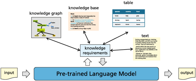

A PLM gets an input text and collects additional knowledge from different sources. This knowledge may be added beforehand or can be retrieved on demand. Subsequently, an output is generated using the additional knowledge

Table 3.9 Models integrating additional knowledge (cf. [166, p. 10]). Benchmarks: GLUE natural language understanding Sect. 4.1.1, TACRED relation extraction Sect. 5.4.2 [199], TriviaQA question answering Sect. 6.2.1 [99], English all word WSD [14], Nat. Quest question answering [109] Sect. 6.1.2

Textual Encoding of Tables::

Often additional knowledge is available in tables. The entries in these tables can be encoded in a special text format. A PLM can be trained with this text to acquire the knowledge in the rows and columns, in a similar way as the relation between the words of two languages can be learned.

Textual Encoding of KB Relations::

An alternative way to use KB information starts with identifying entities or concepts in a text. The relations available for these entities and concepts can be extracted from the KB and can be included in the training process either as text or in another appropriate form.

Adding Retrieved Facts::

When a PLM needs to answer a question or create a text, it can formulate a query on the topic and retrieve corresponding text content from a KB or the Internet. This textual information may be picked up by a transformer and enhance the output. In this way, the model can use comprehensive and up-to-date information on the fly.

Enhancing Logical Consistency::

PLMs sometimes do not generate logically consistent content. By additional fine-tuning tasks a model can be trained to respect logical consistency.

Surveys of methods to incorporate domain knowledge into Deep Neural Networks are given by Dash et al. [45] and Yu et al. [243].

3.4.1 Exploiting Knowledge Base Embeddings

Typically, Knowledge Bases are graph structures where the nodes correspond to entities and the edges represent relations connecting the entities. Many large-scale KBs, such as WordNet [137], YAGO [200], Freebase [18], DBpedia [15], and DiffBot [77] have been released in recent years with millions of entities. Figure 3.13 shows a small subset of the WordNet hierarchy. In most cases a KB can be described by triples (h, r, t), where h and t are entities in a set E, and r is a relation holding between these entities. To assess the semantic contents of a KB, it was proposed to encode its entities as well as its relations as embeddings in a low-dimensional space, allowing to determine the similarity of entities and relations [43]. Subsequently, these embeddings can be used to disambiguate entities (entity linking, Sect. 5.3.3), or predict new relations (Sect. 5.4).

Fig. 3.13

Small part of the WordNet knowledge base describing the relations between English words. It contains synsets of word with approximately the same meaning, which are related by the hypernym (is-a) meronym (has-part) and member-of relations [137]

For the embeddings ) of words generated by Word2Vec [135] it turned out that relations between entities often are represented in the space of word embeddings as vector differences between entity embeddings (Sect. 1.5). An example is the relation between a country and its capital, for which we have approximately ) .

The TransE model [20] is built on this pattern. TransE adapts the embeddings in such a way that whenever (h, r, t) holds and emb(h) and emb(t) are the embeddings of h and t, then equation emb(h) + emb(r) ≈ emb(t) should be approximately valid for some vector emb(r), which is considered as the embedding of the relation r. Consequently, for all triples (h, r, t) in the set S of correct triples the TransE-loss$f_r(h,t)=\left \lVert {emb}(h)+{emb}(r)-{emb}(t)\right \rVert ^2_2$ should become 0. The TransE-model uses the hinge loss to approximate this goal, which modifies the embeddings in such a way that f_r(h, t) for correct relation triples gets lower than $f_r(\tilde {h},\tilde {t})$ for randomly selected incorrect triples $(\tilde {h},r,\tilde {t})$. The models and embeddings are trained with relations from WordNet and Freebase.

There are a number of more elaborate models to encode relations from KBs, as described in the surveys [43, 94]. TransH overcomes TransE’s inability to model complex relations, and TransD aims to reduce the parameters by proposing two different mapping matrices for head and tail. But these alternatives are rarely used for contextual embeddings. Another method for KB representation is tensor factorization [144, 145]. This approach, however, is not based on word embeddings and therefore mainly used for KB completion and not to enhance PLMs.

In the rest of the section we describe approaches, which merge KB-embeddings usually computed by TransE and token embeddings generated by language models. A difficulty is to establish a relation between the token embeddings and the entities, which usually contain several tokens.

KEPLER [224] consists of a BERT-like language model generating token embeddings by the MLM objective. In addition, it computes embeddings for entities from descriptive text in the KB using a special token “<S>” at the beginning of the input text. This token is trained to produce an embedding of the named entity argument of the relation, e.g. for the input “<S> Johannes Kepler” in Fig. 3.14. In this way, the arguments h and t of the relation are embedded. The embedding of the relation r is either a parameter to be trained, or it may be determined by the text verbalizing the relation. These embeddings are fed into the TransE loss and used as an extra training criterion in addition to MLM (Fig. 3.14). In a number of language understanding tasks the approach is able to achieve good results. On the relation extraction benchmark TACRED [254] the approach reaches 71.5% F1-value.

Fig. 3.14

KEPLER [224] trains a conventional BERT-like model by the MLM-loss. For a knowledge base with text entries it generates entity embeddings using the special <S> token and encodes relations by the TransE-loss. Both loss functions are added during training

KnowBERT [157] explicitly models entity spans in the input text and uses an entity linker to retrieve precomputed entity embeddings from a KB to form knowledge enhanced entity-span representations. The KB-embeddings are precomputed with a loss function similar to TransE. Projection mappings are used to transform LM-embeddings to KB-embeddings and vice versa. Information from the best matching KB-embeddings is averaged and retransformed to enhance the LM-embeddings. These computations form an additional layer of BERT. Wikipedia and WordNet were used as KBs. To test KnowBERT’s ability to retrieve facts from the KB, a relation was formulated and one argument of the relation was masked. KnowBERT reaches a mean reciprocal rank (MRR) of 0.31, indicating that on average the correct entity appeared on rank 3, whereas for BERT it shows up on rank 9. Hence, the model generates better answers than BERT, but is only approximately able to reproduce the relations of the KB. However, it often leads to improvements in downstream tasks.

ERNIE-THU [255] relates named entities in a KB to the named entities in a document in a similar way, and transforms embeddings between these two spaces. E-BERT [162] is similar in spirit to KnowBert, but it requires no expensive further pre-training of the BERT encoder. Facts as Experts [213] also links factual information and entities using embeddings, and in this way can inject new information into the model.

In summary the methods presented in this section directly infuse domain-specific knowledge expressed by relation embeddings into token embeddings of PLMs. There are, however, a number of disadvantages. The KB entity embeddings are separately pre-trained with some knowledge embedding models (e.g., TransE [20]) and fixed during training of the PLMs. Thus KB-embedding and token embeddings are not learned simultaneously. Moreover, the KB entity embeddings often cannot fully capture the rich contextual and relational information of an entity in the KB. Furthermore, they are static and do not depend on the context. In addition, they rely to a great extent on the performance of the linking algorithm and on the reliability of graph embeddings. This means that in general other approaches perform better, e.g. for relation extraction (Sect. 5.4).

3.4.2 Pre-trained Language Models for Graph Learning

Relations between objects and concepts can be joined in a graph and provide a uniform representation for the relatedness of many items. Using the structure of a graph many properties of nodes can be predicted. In recent years there was a great effort to design models which can capture the composition of a graph and predict its parts, e.g. node2vec [67] or graph convolutional networks [107]. However, the node representations obtained by such deep models tend to be over-smoothed and also become very vague. PLMs potentially are able to improve the representation by self-attention over long distances. Xia et al. [233] provide a survey on PLMs for graphs. Nodes and edges are characterized by different feature and position embeddings, and are processed with different types of PLMs. Prominent applications are recommender systems exploiting user-product graphs and drug discovery evaluating molecule structures.

Graph-BERT [250] is trained on sample nodes taken from a large graph together with their context. These samples are drawn using the closeness according to the PageRank algorithm [24] and contain no direct link information. Nodes are characterized by feature embeddings, embeddings based on the PageRank information, and hop-based distance embeddings. These embeddings are summarized and form the input of a BERT model. The model is pre-trained to reconstruct the information of masked nodes and to predict the relation between two nodes by evaluating their cosine similarity. The model is fine-tuned for node classification and graph clustering. Graph-BERT achieves the second-best accuracies for node classification on three graph benchmarks [128, p. 16].

GPT-GNN [87] proposes an autoregressive PLM to perform an iterative reconstruction on given graphs. The method assumes a random order on the edges and nodes. Given the edges and nodes up to a specific position, it predicts the properties of the next nodes/edges. GPT-GNN generates one masked node and its edges at a time and optimizes the parameterized models via maximizing the likelihood of the node and edges generated in the current iteration. Then, it iteratively generates nodes and edges until all masked nodes are generated. The model is trained on a graph of 178M scientific papers with their features, the venue and the authors, and on a graph with 83M Amazon reviews, users and products. On both benchmarks the model has the best accuracies.

MPG [120] consists of a BERT model encoding node and edge features. As a pre-training task, the model has to learn whether two graphs divided into two halves actually belong together or whether the halves are a random pair. The model is applied to the modeling of molecules and achieves Sota results on a range of 14 benchmarks, especially drug discovery.

GraphFormers [238] jointly models a graph structure together with sequences of words. Each node of the graph contains a text. A center node and its neighbors are tokenized into sequences of tokens. The model has special transformer layers for computing the embeddings of text tokens and for the derivation of node embeddings by aggregating the corresponding text embeddings. The model is pre-trained with the task to predict, if two nodes are linked or not. GraphFormers is tested on three benchmark tasks, e.g. a graph with scientific papers characterized by their titles and their citation graph. The model consistently outperforms all prior approaches in the prediction of links.

3.4.3 Textual Encoding of Tables

Tabular data probably makes up the majority of all business and administrative data today. Examples are retail transactions, official statistics, processing data from industrial applications, etc. A survey on the interpretation of tables on the web is provided by de Alwis et al. [46]. Previous work often relies on manually selected features, cannot handle the flexible schemas in web tables, and does not generalize well across tasks.

TURL [47] characterizes a relational table by the table caption C (a short text, may be enhanced by section title), column headers h_i (a sequence of tokens) describing the table scheme H = {h₁, …, h_m} and cell values, where each cell may represent an entity, e.g. a person. Cells in the same row share some relation, and cells in the same column share another relation. This requires a structure-aware attention mechanism implemented by a visibility matrix, which restricts the attention to specific columns and rows.

TURL is pre-trained according to the masked language model loss on a large unstructured dataset consisting of the table captions and headers. Subsequently, the relation between entities in the same row or column can be learned. Entities in a table are masked, and the model has the task to predict them based on the table context and the visibility matrix. By this target TURL can learn factual relations from the table and encode them into entity embeddings (Fig. 3.15).

Fig. 3.15

Learning table relations with TURL [47]. On the left side the table caption and the column headers are trained. On the right side the row markers together with input entities (cells in a specific row) are processed

The model is trained on 570k tables extracted from Wikipedia. All columns containing at least one linked cell are marked as entity columns. After fine-tuning, the model is able to predict the masked contents of table cells in the test set with precision of 54.8%, beating competing approaches. An ablation study shows that the visibility attention matrix is essential for achieving a high performance.

TaBERT [241] aims to include both, natural language text and structured table data. TaBERT is trained on 26.6M tables and surrounding text from English Wikipedia and the WDC WebTable Corpus [115]. Each table cell is described as (column header, column value type, value). Subsequently, the table rows are encoded as text, as shown in Fig. 3.16. For pre-training 20% of the columns of a table are randomly selected and the model has to predict the masked column names and types. In addition, the cell values are reconstructed according to a special scheme. The model is fine-tuned on the WikiTableQuestions benchmark [155], which contains questions requiring compositional, multi-hop reasoning over a series of entries in the given table. To reduce effort only table rows containing query tokens are encoded. TaBERT is able to increase the Sota accuracy on this benchmark to 51.8%. The authors show that their table cell encoding is more effective than alternatives. RPT [205] proposes a similar scheme for table encoding. BRIDGE [124] is a system for semantic parsing, which converts information from text and tables to an SQL query extracting information from a database.

Fig. 3.16

TaBERT [241] encodes the rows of a table as text in a special format. The “context” contains corresponding text. Each table cell is represented as (column header, column value type, value). Here the first table row is encoded by the line starting with [CLS]

Tapas [81] is a variant of BERT optimized for table processing. The table is flattened row-by-row, tokenized and enhanced with position embeddings. Following embeddings are added: a row id embedding, a column id embedding, and a rank embedding indicating the rank in the sorted sequence, e.g. for numbers. The model is pre-trained on 6.2M table-text pairs from the English Wikipedia with the task to restore words in both table and text that have been replaced with a mask. The model can do this with relatively high accuracy (71.4% accuracy on a test set).

During fine-tuning the model learns to answer questions from a table, e.g. “Which wrestler had the most number of reigns?” for a table with wrestling results. [CLS] and a query are prepended to the flattened table and both parts are distinguished by an additional segment embedding. The model has two output types: (1) a score for each table cell with the probability that this cell will be part of the answer and (2) a probability of the result type (none, count, sum, average) for [CLS] to produce the final answer. Together the result indicates which operation should be performed over which table cells to generate the final answer. On several benchmarks Tapas reaches Sota results, e.g. improving from 55.1% to 67.2% for SQA benchmark [90]. The source code and pre-trained models are available at Hugging Face.

The results show that the models described above are able to extract information from tables and answer question about the table content. This makes it possible to use a large source of information, since tables are ubiquitous in text documents and web pages. In principle, the approach can also be used by large Foundation Models to include table information in the text they generate.

TableGPT [63] generate a text from a table using the GPT-2 language model. It enhances GPT-2 for table-to-text generation with two auxiliary tasks, table structure reconstruction and content matching, for improving text fidelity.

3.4.4 Textual Encoding of Knowledge Base Relations

A number of proposals try to verbalize KB-relations as text. In this way, KB-relations may be directly incorporated in the training text of the language models.

WKLM [234] randomly replaces a fraction of the entity mentions in the original document with names of other entities of the same type. The model is trained to distinguish the correct entity mention from the randomly chosen ones. In addition, the model has to predict masked token. The types of entities are obtained from Wikidata [214]. In this way, the model can better capture entity information from natural language and yields better results for entity-related NLP tasks. WKLM is able to predict relation arguments much better than BERT. In question answering (SQuAD and open domain, Sect. 6.2) the model is also able to reach Sota results. Similar approaches [191, 203, 234] propose entity and phrase masking and replacement schemes.

CoLAKE [202] extracts the knowledge context of an entity from large-scale knowledge bases. The model links entity mentions to the underlying entities in a KB by an entity linker. The mention nodes are then replaced by their linked entities. The CoLAKE model is initialized with the RoBERTa_BASE model. It is trained on Wikipedia with 3 million entity embeddings and 822 relation embeddings aligned to the Wikidata5M KB [224] on 26M training samples. The example input “[CLS] Harry Potter points his wand at Lord Voldemort [SEP]” is shown in Fig. 3.17. The type of inputs (word, entity, relation) is encoded as type embeddings and added to the token and position embeddings. To introduce a relation from the KB, e.g. “(Harry Potter, mother, Lily Potter)”, the relation node “mother” and the entity node “Lily Potter” are introduced with the position embeddings 2 and 3, as the first relation argument “Harry Potter” is located at position 1. Self attention is computed between text inputs. There is a masking mechanism restricting the self-attention for relation elements, e.g. to the pairs “(Harry Potter, mother)” as well as “(mother, Lily Potter)” in our example.

Fig. 3.17

CoLAKE [202] identifies entities and encodes them with specific embeddings. Type embeddings distinguish words, entities and relations. The input embeddings are the sum of token/entity, position, and type embeddings. For all entities in the input text relations are extracted from the Knowledge Base and appended after “[SEP]”, e.g. mother(Harry Potter, Lily Potter). A masking mechanism ensures that relation elements can attend only to their corresponding elements in the input text. During pre-training the model has to predict masked tokens and entities

During pre-training about 15% of the input elements (words, entities, relations) are masked and have to be predicted by the model. As entity nodes simultaneously appear in the input text and the knowledge base this helps to align the representations of language and relations. Masking relation nodes helps CoLAKE to learn contextualized representation for relations. On the language understanding tasks of GLUE the CoLAKE model achieves a similar average of 86.3 as RoBERTa. An alternative task consist of the completion of relation triplets (h, r, t) using a sentence describing the relation. It turns out that CoLAKE is much better than its competitors, e.g. the correct relation is inferred from two entities in 72.1% of the cases.

LUKE [237] treats words and entities in a given text as independent tokens, and outputs contextualized representations of both. The model is based on BERT and trained to predict randomly masked words and entities in a large entity-annotated corpus derived from Wikipedia. It contains an entity-aware self-attention mechanism that is an extension of BERT’s self-attention. It takes into account embeddings indicating if a token represents text or an entity. LUKE yields Sota results in relation classification, entity typing and NER. K-adapter [222] is a related approach using RoBERTa (Sect. 3.1.1) as fixed background model and building several independent “Adapters” to include knowledge from different KBs.

EWISER [14] similarly targets word sense disambiguation (WSD). Starting with BERT embeddings, it computes scores for WordNet synsets (sets of words with similar meaning). Exploiting the interdependence of the synset graph the approach computes final scores that a word belongs to a synset. It achieves a new Sota on a number of WSD benchmarks (Sect. 5.2).

PET (Pattern-Exploiting Training) [184] as an alternative constructs an additional training set using only a few labeled examples. Consider a 5-star scale rating for a restaurant in the Yelp dataset [185]. The authors add text to the reviews to express the ratings, e.g. “All in all it was great”. Using this approach the authors convert the Yelp dataset to a task for predicting masked words, e.g. “All in all it was [MASK]”. However, they provide the verbalized labels only for a small number of examples. Subsequently, they predict the best class for the non-labeled examples and train the model with the predicted classes as well as the language modeling loss to avoid catastrophic forgetting. This can be done in several iterations. Although only a few labels have been used, the model performs better on Yelp than standard supervised approaches. The SuperGLUE benchmark data covers eight challenging NLP tasks. With just 32 labeled examples the PET approach trained according to the above schema yields a better average (75.4%) than GPT-3 (71.8%) with the same number of few-shot examples. This shows that good results can be achieved with a small model (223M) and only few labeled examples. Note that the fine-trained Sota for SuperGLUE is 90.4% using T5 and Meena.

TeKGen [1] is a data-to-text sequence-to-sequence model to verbalize a complete KB. It is applied to the English Wikidata knowledge base [214] with ≈ 6M entities and about 1500 relations. The model starts with a large training corpus of heuristically aligned Wikipedia text and Wikidata triples. Relations sharing a common entity subject are converted to the input subject relation₁object₁, …, relation_nobject_n for the T5 transformer (Sect. 3.1.3). As an example “To kill a Mockingbird, author: Harper Lee, publication date: 11 July 1960” is translated to “To Kill a Mockingbird is a novel by Harper Lee published in 1960.” The T5 model is fine-tuned and subjected to an addition check to generate good verbalizations. The resulting dataset of verbalized triples was used in a question answering task. It was able to increase the accuracy in theNatural QuestionsNatural Questions (NQ) benchmark [109] (Sect. 6.1.2) from 38.8% to 41.5%. KGPT [30] in a similar way converts structural knowledge into the serialized text and lets model learn knowledge-text alignments.

In summary these methods transform KB relations into text, e.g. as complete sentences expressing relations or as concatenated triples (e.g., [head text, relation text, tail text]) into LMs for training or fine-tuning. This text is transformed into contextual embeddings and the model is trained to detect the underlying relation. The drawback is that focusing on knowledge base completion tends to over-adapt the models to this specific task, which comes at the cost of generalization.

3.4.5 Enhancing Pre-trained Language Models by Retrieved Texts

An open domain question answering system has the task of answering questions not restricted to a specific domain [27]. Consider the following example from the TriviaQA benchmark [99]. “Question: The Dodecanese Campaign of WWII that was an attempt by the Allied forces to capture islands in the Aegean Sea was the inspiration for which acclaimed 1961 commando film?”“Answer: The Guns of Navarone”. It is not plausible that the model can reproduce such a specific response from the knowledge stored in its parameters, even if it was present in the data before training. Therefore, it would be desirable for the system to be able to gather additional evidence by a retriever collecting relevant documents from a large text repository. Subsequently, it has to align the retrieved information with the question and generate an answer by another PLM, a reader. New web search techniques can be used for this approach. They are based on comparing embeddings for words or passages consisting of several sentences. There are numerous applications such as question answering, summarization, and dialog systems. In Sect. 6.1 this is discussed in more detail. Recent surveys are provided by Zhu et al. [259] and Yu et al. [244].

DPR (Dense Passage Retriever) [103] employs a PLM to encode KB-passages d_i, e.g. from Wikipedia, as embeddings emb(d_i). This can be achieved by fine-tuning a BERT model to encode passages by the embedding of the token [CLS]. These embeddings can be stored in an index for fast access. Then the DPR retriever processes the query sequence x by another BERT model and generates the query embedding emb(x). A number of k = 100 passages d_j with maximal inner product ${emb}(x)^\intercal {emb}(d_j)$ is retrieved by a nearest-neighbor search. Both BERT encoders can be trained together to generate appropriate embeddings using weak supervision in the form of question-answer pairs (cf. Sect. 6.1.5). If, for instance, the query is “Who is the bad guy in lord of the rings”, the algorithm can retrieve “Sala Baker is best known for portraying the villain Sauron in the Lord of the Rings trilogy”, because “bad guy” and “villain” have similar embeddings. Therefore, DPR can find passages with similar meaning, expressed with different words. Karpukhin et al. [103], for instance, show that already with 1000 training examples the dense retriever is better than the classical keyword search. For 40k training examples the top-20 retrieved passages contain the correct answer in about 79% of the time, while this value is only 59% for the classical retrieval. An in-depth discussion is given in Sect. 6.1.5.

The DPR reader is another BERT model. Similar to BERT’s text pair classification, it is fine-tuned to predict a probability for each retrieved passage that this passage contains the correct answer. In addition, it selects a span of tokens by span prediction, which probably provides the answer. In the example it selects “Sala Baker” as the answer. Together both components form a retriever-reader architecture, which recently became popular. The approach can be easily applied to KBs with billions of passages [103, 201]. On the Natural Questions [109] it yields a test set accuracy of 41.5%.

DensePhrases is a different system creating embeddings for phrases of up to 20 words in the KB, which are computed without knowing the query [114]. The processing of the retrieved phrases directly yields the answer without much computational effort. Using careful workflow optimization the authors achieve near-Sota results with a much lower processing time than dense passage retrieval systems, e.g. a test set accuracy of 40.9% on Natural Questions.

FiD (Fusion in Decoder) [91] employs DPR as retriever. In the reader step it uses the special tokens “question:”, “title:”, and “context:”. These tokens mark the question, the retrieved passage title and the passage text and are concatenated forming the input. Subsequently, these k retrieved triples are fed one-by-one into a transformer encoder like T5 [170] (770M parameters), which independently processes each triples by the encoder. Only in the decoder the passages are handled jointly and the text of the answer is generated. This approach drastically reduces the computational effort. The transformer is fine-tuned on a QA-task. The architecture of the model is shown in Fig. 3.18. Raffel et al. [170] provided evidence that generative models like T5 are even competitive for QA-tasks such as SQuAD [173], where answers are spans in a given document.

Fig. 3.18

A retrieval enhanced language model [91] encodes the query and the KB passages as embeddings and uses a pre-trained retriever to find passages corresponding to the query. The reader is a Seq2seq model (T5) combining the query and the passages to generate the answer. This model setup is fine-tuned with different benchmark datasets

The system achieves a test set exact match accuracy of 51.4% on the Natural Questions benchmark compared to 41.5% for DPR. The TriviaQA benchmark [99] contains a set of trivia questions with answers that were originally scraped from the Web. On this benchmark the model yields Sota results with 80.1% exact match accuracy [211]. This is better than the accuracy of other much larger models, like GPT3 with 175B parameters (71.2% EM), or T5 without retrieval and 11B parameters (60.5% EM). It turns out that increasing the number of retrieved passages strongly enhances the answer quality.

There are a number of new approaches to augment PLMs with text from an external KB. In Sect. 6.1 we describe different PLMs for retrieval that can be used by web search engines. In Sect. 6.2 we investigate systems for question answering that often employ a PLM-based retrieval mechanism and an additional PLM to generate the answer text. It combines the query, the knowledge acquired during training, as well as the information in the retrieved documents.

In summary, combining language models with retrieval is currently the most efficient way to incorporate additional information into PLMs. The new information is focused on the current query and thus very informative. The retrieval model can access semantically related passages within fractions of a second using new approximate open-source nearest neighbor index structures. By relying on embeddings, synonyms and paraphrases can be found and the meaning of words can be disambiguated. In addition, the underlying knowledge bases can be updated on the fly to keep the information current.

3.4.6 Summary

The knowledge covered by the textual training data can be leveraged in various ways to improve the performance of PLMs. Entities and relations from a knowledge base can be represented by embeddings, e.g. by TransE. However, the utilization of these embeddings for PLMs is not very efficient and error-prone. A more promising alternative is the direct use of table content or knowledge base relations by specialized PLMs, which capture relationships between entities and table cells by specific self-attention patterns. Similar to Graph-CNNs PLMs have been directly used to acquire the relationship between the nodes of a graph by encoding the features of links by embeddings in a BERT-like model. Along this line a promising way to transfer relational knowledge from a graph to a language model is proposed by GraphFormers.

A very simple and efficient approach of incorporating tables and knowledge bases in PLMs is the creation of text that expresses the information content. This can be used by the PLM either as conditioning text or during training. However, the most promising way to include knowledge is retrieval, since most information is stored in the form of unstructured text on the Web or databases. Here, the retriever-reader architecture emerged as an effective way to collect relevant passages. Subsequently, the PLM generates new text by combining the internal knowledge, the start text, and the retrieved passages.

Much effort was devoted to the extension of the length of input sequences (Sect. 3.2). This was mainly achieved by sparse attention patterns reducing the increase in computational effort from quadratic to linear with S4 as a leading approach. Nevertheless, larger input sequences still have limited range of context both within the same sample and outside of it.

In contrast, retrieval can cover an indefinite context within the same sample by gathering appropriate passages, even if there is no simultaneous attention over the whole context. In addition, retrieval can access relevant information in huge document collections. Either the highly developed traditional keyword search engines may be used. Alternatively dense retrieval may be employed which compares embeddings of the query and passages using approximate nearest neighbor search over an index. It turns out that relatively small retrieval-based models outperform large Foundation Models like GPT-3. FiD, for example, achieves an exact match accuracy of 51.4% on the Natural Questions benchmark compared to 29.9% for GPT-3. Retrieval is extensively used by recent models such as WebGPT and Retro.

3.5 Changing Model Size

The size of a model, especially its number of parameters, has a marked influence on the performance of the model, its memory requirements and the computational resources required for training. In the first section we discuss that models with more parameters potentially have a better performance. This, however, requires a larger computational effort during training and model utilization. An alternative are mixture-of-experts models, which define a number of parallel model structures which selectively compute a solution. This is described in the second section.

As initial versions of successful models often are extremely large, a variety of model compression and acceleration techniques have been developed. They reduce memory requirements and training time without noticeable degradation of accuracy, and allow the models to be deployed on low resource computing devices, such as cell phones. There are three main techniques for model size reduction [65]—parameter compression and reduction, low-rank factorization, and knowledge distillation—which are outlined in the subsequent sections.

3.5.1 Larger Models Usually Have a better Performance

As a rule for machine learning, the number of parameters of a model should be limited to avoid overfitting, i.e. adapting to random fluctuations in the data. It turned out that this does not hold for PLMs if the amount of training data and the number of model parameters are increased simultaneously. Larger PLMs have been shown to have better performance on NLP tasks, which is underscored by theoretical work on PLMs [19, p. 117]. The benefits of increasing the number of parameters come from two factors: additional computations at training and inference time, and increased memorization of the training data. Kaplan et al. [102] empirically investigated in detail the dependency between the number of model parameters R (excluding embeddings), the size N of the training data, and the amount of computing effort C used for training. They evaluated a large number of models and draw the following conclusions:

• The performance of the models depends largely on the size quantities R, N, C. Other architectural features such as width or depth have only a weak influence.

• The performance follows a smooth power-law dependency with each of R, N, C, if the other quantities are not too small. As an example the loss is approximately L ≈ (N∕(5.4 ∗ 10¹³))^−0.095.

• If R and N are increased at the same rate, the model accuracy grows reliably. If one of these factors is held constant the improvement gets lower. To get the best performance, the model size R should grow with the factor 8, if the data N is increased 5 times.

• Training loss has a predictable dependency on computing effort and can be extrapolated.

• The performance of fine-tuning of a pre-trained model on a different training task depends strongly on the loss for the pre-training validation set. Therefore, transfer to a different distribution induces a constant penalty, but roughly improves with the performance on the pre-training set.

• Large models are better able to extract information from data than small models. They reach the same level of accuracy with fewer optimization steps and using fewer data points. If there is only a fixed amount of computation time, but no restrictions on size or data, one should use very large models and stop before convergence (Fig. 3.19). The optimal batch size depends on the gradient noise, which is easy to measure during training [132] and is larger than assumed before.

  Fig. 3.19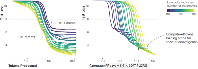

  

  A series of language model training runs with varying model sizes [102]. The left graph shows that larger models require fewer samples to reach a fixed test loss. The right graph demonstrates that the model size should grow with compute budget. Image reprinted with kind permission of the authors [102, p. 4]

These findings show that the success of larger PLMs is a systematic feature. A larger number of model parameters is much more sample efficient than thought before, when overfitting was a major problem for smaller training tasks. This also explains the success of large models like T5, BigBird, or GPT-3. Hernandez et al. [80] investigate empirical scaling laws for the transfer from pre-training to fine-tuning. Figure 3.20 plots the training efforts of some Deep Learning models during the last two decades.

Fig. 3.20

Number of parameters for Deep Learning Models since 2017 [188]. Note that the parameter scale is logarithmic. The number of parameters roughly increased from 100M up to 1000B

3.5.2 Mixture-of-Experts Models

As discussed above a model with more parameters usually can achieve a better performance. A simple way to increase the number of parameters without a higher training effort is a mixture-of-experts architecture. It was already proposed in the nineties by Nowlan et al. [147] and has a strong resemblance to decision tree models [152]. It consists of a single gating module and a number of expert modules with identical architecture but different parameters. Each expert specializes in only a subset of the data, and the gating module assigns each input to the appropriate experts. Specifically, the gating network computes a probability distribution over the experts indicating how well each expert is able to process the incoming input. A reduction in computational effort can be achieved, if only a few expert modules are actually used. The model is trained by stochastic gradient descent, which can compute the parameter gradient despite the discontinuities if some expert is exchanged. Increasing the number of experts keeps the computational cost constant because the model always selects the same small number of experts for each input, regardless of the total number of experts. The architecture enables massive models and is particularly efficient for distributed systems where the experts are spread across different computational devices.

Clark et al. [38] analyze the theoretical properties of such routing networks, where each input is processed only by subnetworks with a fraction of the network’s parameters.The authors analyze three different architectures and get the following results.

• Routing improves the performance of PLMs in all investigated sizes and variants.

• Improvement follows a power-law in the number of experts E that diminishes with model size N, and can be further generalized across routing architectures.

The analysis is based on the evaluation of several magnitudes of size, including models with hundreds of experts and hundreds of billions of parameters.

GLaM [51] is an autoregressive mixture-of-experts (MoE) model with up to 1200B parameters. It replaces the fully connected layer of every second encoder block (Sect. 2.1.1) with 64 copies having different parameters. For each embedding, a gating module selects two of these 64 fully connected layer for processing. The architecture is shown in Fig. 3.21. The model was trained on a huge collection of 1.6T tokens documents and quality-checked web pages. It has approximately 7 times more parameters than GPT-3 but requires only 1/3 of its training effort. In this way, the model has many more parameters increasing its representational capacity. As for a given input token, only two expert models are used, the computational effort for training and application is lower. The zero-shot and one-shot performance is better than for GPT-3 on 29 NLP tasks. Some results are compared to those of other models in Tables 3.3 and 3.4. GLaM is remarkable as it requires only 1/3 of the training effort of GPT-3 but it achieves a similar or better performance than GPT-3 on NLP tasks.

Fig. 3.21

Architecture of GLaM [51]. For each input token, e.g., “likes”, the gating module dynamically selects two most relevant experts out of 64 available experts. This is indicated by the blue grid. The weighted average of the outputs from these two experts’ feedforward models is then passed to the next encoder block. For the other inputs different experts are selected. A mixture-of-experts layer is used in every second encoder block

WuDao-2.0 [175, 178, 257] is a recent giant autoregressive language model with 1750B parameters, ten times larger than GPT-3. It has mixture-of-experts layers, where a gating network selects a submodule for processing based on the input. WuDao-2.0 uses the FastMoE library [74] and employs the GLM 2.0 architecture (Sect. 3.1.3) combining the different learning paradigms of BERT, GPT and the encoder-decoder transformer [175].

The training data consist of 1.2TB Chinese text, 2.5TB Chinese graphic data and 1.2TB English text data from the Pile corpus [61]. The Cogview model is used for the joint processing of images Sect. 7.2. In addition, WuDao-2.0 can learn on the fly, draw pictures and compose poetry. These capabilities are a significant difference to GPT-3.

The published performance claims are impressive. On the LAMA benchmark for measuring world knowledge [158] it scores higher than AutoPrompt [192]. For the SuperGLUE few-shot natural language understanding task [219] it achieves Sota and surpasses GPT-3. For the Lambada benchmark (Sect. 4.1.3), where the last word of a paragraph has to be predicted, it yields better results than Microsoft Turing NLG. In addition, it increases Sota for a number of text-graphics tasks (Sect. 7.2.8).

Switch [56] is a variant of the transformer encoder-decoder T5 (Sect. 3.1.3). It has a mixture-of-experts architecture, which replaces the fully connected layer of each encoder block with k = 128 copies having different parameters. There is a simple linear gating network, which selects one of the 128 single fully connected layers (the experts) per token. Hence, the number of parameters is drastically increased with approximately constant computational effort. For this architecture a gradient can be computed and the model may be optimized using a number of specific strategies and a special TensorFlow version. It turns out that Switch achieves the same loss level compared to the standard T5 version with 1/7 of the computing time. On a number of fine-tuning tasks the large Switch model with 1600B parameters and 2048 experts yields better results than T5-large (Sect. 3.1.3) with 13B parameters requiring a quarter of the computational training effort.

As an alternative to the gating network in the mixtures-of-experts architecture, it is possible to use hash values to activate different parts of the network. Token Switch [177] computes a hash value for each input token and routes the generated embeddings of each token to different feedforward networks based on the hash values. The authors show that their approach compares favorable to Switch and works well on comprehensive language modeling tasks.

ST-MoE-32B [261] is a mixture-of-experts model with 269B parameters and a comparable training cost of a 32B dense model. The authors modify the routing algorithm which dispatches token embeddings to one or two experts, and resolve instability issues. The model is similar to a T5-Large encoder-decoder [170]. The ST-MoE-32B has 32 experts with an expert layer frequency of 1/4, such that every fourth feedforward layer of T5 is replaced by an MoE layer. The authors use the GEGLU activation function, which contains multiplicative elements [142]

$$\displaystyle \begin{aligned} FFN_{GEGLU}({\boldsymbol{x}},W,V,{\boldsymbol{b}},\boldsymbol{c}) = GELU({\boldsymbol{x}} W+{\boldsymbol{b}})\odot ({\boldsymbol{x}} V+\boldsymbol{c}). \end{aligned} $$

(3.2)

The authors compare a large number of variants and hyperparameters to improve training.

The model achieves Sota in many transfer learning benchmarks, e.g. for SuperGLUE with an average accuracy of 93.2% beating the PaLM LM with 540B parameters. Other Sota results were reached for summarization (XSum [143] with 27.1 Rouge-2, CNN/Daily Mail [78] with 21.7 Rouge-2), closed book question answering (WebQA [13] 47.4% exact match, Natural Questions [109] 41.9% exact match), and adversarially constructed tasks for common sense reasoning (Winogrande [182] 96.6%, ANLI R3 [146] 74.4%).

3.5.3 Parameter Compression and Reduction

Model quantization is a parameter reduction technique, where parameters are stored in low precision and therefore the computations in PLMs are also less precise. Conventional models normally use parameters of 32 bits or 16 bits, while parameters after quantization can have 8 bits or even 1 or 2 bits. Q-BERT [190], for example, quantizes Transformer models to ultra-low precision. This reduces the model size 13-fold while only loosing 2.3% performance. The authors avoid the naive approach of simply reducing weight precision, but use additional training steps to adjust the quantized weights and allow higher precision for more “sensitive” parameters. Other authors propose to delete parameters with small values [64]. ALBERT [113] uses the same weights across all layers and achieves a significant parameter reduction. Nevertheless, ALBERT has the same or better performance compared to BERT.

Another approach aims to reduce the number of parameters, e.g. by removing attention heads. It was shown that most attention heads focus only on nearly identical positional relations and can be replaced with fixed attention patterns [172]. It turned out that high performance is possible with only 1–2 attention heads per encoder unit instead of the 16 attention heads of the original model. A detailed overview on parameter compression techniques is provided by Ganesh et al. [60] .

Another method to reduce model parameters is model pruning, which cuts off irrelevant parts in PLMs to achieve a smaller memory footprint and faster execution without compromising performance. It could be shown, for example that some attention heads of the transformer may be removed with little impact on the accuracy [256]. Other researchers prune the weights of attention layers and linear layers to reduce the number of parameters without reducing the accuracy [29, 64]. Note that model pruning does not always lead to speedups, as sparse computations may be hard to parallelize on GPUs.

3.5.4 Low-Rank Factorization

This technique employs matrix and tensor decomposition to reduce the number of parameters of full rank parameter matrices and already has been discussed in Sect. 3.2.2 for the extension of the input sequence length. Examples are the Performer [34] and the Linear Transformer [105] (Sect. 3.2.2). As an alternative, ALBERT (Sect. 3.1.1) approximates the embedding matrix as a product of two smaller matrices.

3.5.5 Knowledge Distillation

In machine learning the knowledge distillation approach [82] transfers knowledge from a large teacher model to a smaller student model. The large model can often be trained successfully to approximate a functional relation without using its full representational capacity. To reduce the high computational and memory requirements during application, a smaller model is trained to imitate the large model without sacrificing accuracy.

The advantage of this approach is that the student model may be trained to approximate internal activations of the teacher model. Often the target probabilities generated by the teacher model are used to train the student network . Typically the outputs of the teacher model for an input x is z(x), which can be translated to a probability by a scaled softmax

$$\displaystyle \begin{aligned} {\boldsymbol{y}}(x|\tau) = \frac{[\exp(z_1({\boldsymbol{x}})/\tau),\ldots,\exp(z_k({\boldsymbol{x}}))/\tau]} {\exp(z_1({\boldsymbol{x}})/\tau)+\cdots+\exp(z_k({\boldsymbol{x}})/\tau)} , \end{aligned} $$

(3.3)

where y(x|τ) is a probability vector and τ is a parameter called temperature, which for a standard softmax is normally set to 1.0. The student model is trained to imitate the probabilities $\hat {{\boldsymbol {y}}}(x|\tau )$ generated by the teacher model by minimizing cross entropy

$$\displaystyle \begin{aligned} E({\boldsymbol{y}}|\tau) = - \sum_{j=1}^k \hat{y}_j(x|\tau)\log y_j(x|\tau), \end{aligned} $$

(3.4)

where y(x|τ) is the output probability vector of the student model. If observed values are available the probabilities of the teacher model y_j(x|τ) may be replaced by 1.0 for the observed class and 0.0 otherwise. During training the temperature may be varied. A high temperature avoids extreme probability values and reduces the gradients. This may lead to a faster convergence in the beginning of the optimization.

DistilBERT [183] uses MLM cross-entropy loss to predict token probabilities and in addition the cosine similarity between the embedding matrices of the teacher and student networks to train a smaller BERT model. It utilizes knowledge distillation during pre-training to reduce the size of BERT by 40% while retaining 99% of its original capabilities and making the inference 60% faster. MobileBERT [204] is based on a specific large BERT model and transfers information about multi-head-attention as well as the resulting embeddings. Experiments show that MobileBERT is 4.3× smaller and 5.5× faster than BERT while achieving competitive results on well-known benchmarks.

TinyBERT [97] proposes distillation of a BERT model during pre-training and fine-tuning. The model is adapted to: (1) the output of the embedding of selected layers; (2) the hidden states and attention matrices derived from selected Transformer layers; (3) the logit outputs of the prediction layer. As distillation is also performed during fine-tuning the model can be better adapted to the fine-tuned BERT. On a number of benchmarks TinyBERT is on par with BERT_BASE and outperforms DistilBERT.

Note that the knowledge distillation methods discussed above require the data used for pre-training the teacher model, which is often not released because of data copyright. It has not yet been evaluated whether distillation is also feasible with new data. The training time for knowledge distillation is high, because the teacher model needs to perform a forward prediction over the entire pre-training data to generate activation values or intermediate representations.

Rogers et al. [176] list a large number of size reduction studies for BERT and report parameter size and computing time reduction as well as the resulting performance. For a number of approaches there is a marked reduction in memory and computing effort with nearly identical performance.

3.5.6 Summary

The number of model parameters, the size of the training data and the amount of computation effort for training are the determining factors for the performance of a model. Kaplan et al. [102] show by experiments that increasing parameter count and training set size reliably lead to a better performance and provide a detailed formula for the dependency. If a fixed compute budget is available, one should use a very large model and much data.

Mixtures-of-experts follow this approach by increasing the number of parameters without requiring more computational effort. By routing inputs to specific subnetworks they are able to increase performance compared to monolithic networks. Examples are GLaM, WuDao-2.0, and Switch. However, these networks have hundreds of billions of parameters and require a specific parallel computational infrastructure.

Often the trained networks are too large and have to be reduced to fit to smaller computing devices. A viable approach is low-precision computation, which reduces memory requirements for parameter storing. Low-Rank factorization of matrices also has a lower memory footprint as a side effect. Finally, knowledge distillation may be employed to create a student model which imitates the inner working of a large trained teacher network. DistilBERT, for example, was able to reduce the memory size by 40%, kept 99% of the original performance and was 60% faster. There are a number of other size reduction approaches with similar results.

3.6 Fine-Tuning for Specific Applications

Self-supervised pre-training of language models on large text collections and subsequent fine-tuning them to solve specific tasks has become the standard paradigm in natural language processing and understanding. It has been shown that pre-trained language models such as BERT are excellent for generalization and can easily be fine-tuned to multiple tasks. However, sometimes simple fine-tuning to a domain-specific task is not sufficient, and other transfer learning approaches have to be used to better adapt models to domain-shift in the data [166]. There are a number of surveys covering transfer learning in depth [230, 252, 260]

Fine-tuning updates all the model layers, including the embedding layer, but there are larger changes in the higher layers [133]. First, we discuss whether fine-tuning can destroy the knowledge gained during pre-training. Standard fine-tuning adapts a large pre-trained PLM with many parameters to a relatively small fine-tuning training data set with little computational effort. We investigate whether overfitting occurs during this phase. Subsequent sections introduce different approaches for fine-tuning:

• Intermediate Fine-Tuning performs an in-between fine-tuning step with a larger training set before a final target fine-tuning takes place.

• Multitask fine-tuning enhances the model capabilities by simultaneously fine-tuning on a number of tasks.

• Fine-tuning a frozen model adapts a small additional layer to the fine-tuning task instead of changing all weights of the large pre-trained model.

• Creating Prompts for Few-Shot Instructions aims to generate inputs for a large autoregressive PLM like GPT-3 to solve a task in a zero or few-shot approach.

3.6.1 Properties of Fine-Tuning

Fine-tuning of PLMs is commonly employed to adapt a pre-trained model to a specific task by supervised training. This adaption of the model from a source task to a related target task is also called transfer learning. Transfer learning is especially rewarding if we have abundant training data for self-supervised learning—as it is typical for non-annotated text—and only little annotated data for the target task. A survey of transfer learning is provided by Zhuang et al. [260]. Fine-tuning has a number of advantages:

• The model acquires detailed knowledge about the language, its syntax and semantics by exploiting the content provided in the pre-training data.

• Pre-trained models can easily be adapted to new tasks, e.g. by an additional layer with a simple classifier. The language representations of the pre-trained model support fine-tuning and are only slightly changed during this process.

• Fine-tuning even with a small data set yields a much better performance than direct training of a classifier on the limited data.

Autoencoder models like BERT are typically fine-tuned for classification tasks, where the logistic classifiers for masked language modeling and next sentence prediction have to be removed. Using the [CLS] token or other tokens as input, new logistic classifier models as well as all model parameters are trained end-to-end with the new task for a few epochs (Sect. 2.1.3). Compared to pre-training, fine-tuning is relatively inexpensive. Usually, only a small fraction of the pre-training effort is required to achieve good results.

Tripuraneni et al. [210] have theoretically proven that transfer learning requires far less data than learn tasks in isolation. They prove that transfer learning improves if the task diversity is enhanced. Bansal et al. [7] investigate the theoretical properties of fine-tuning a classifier using pre-trained embeddings. The authors prove that these classifiers have a smaller generalization gap between their train and test accuracy, than standard classifiers.

3.6.1.1 Catastrophic Forgetting

The question is whether fine-tuning can destroy the original capabilities of the model. This means, after fine-tuning a pre-trained model for a few epochs, it could lose predictive performance available after pre-training. A possible reason can be catastrophic forgetting, where all parameters are adapted to a new learning task while forgetting learned content.

Merchant et al. [133] fine-tune BERT_BASE with three different tasks: (1) MNLI sentence pair classification task [229] measuring if the first sentence entails the second; (2) SQuAD question answering [173], where the answer to a question has to be marked in a text; (3) Dependency Parsing [50] to capture the syntactic structure of sentences. Then they investigate the performance of a number of probing classifiers before and after fine-tuning. The results demonstrate that the fine-tuned models only show a small decrease in the accuracy to detect linguistic concepts. The reduction cause by the MNLI task in most cases is less than 1%, while higher differences (less than 3%) are observed for SQuAD and dependency parsing. Therefore, catastrophic forgetting cannot be observed. The authors state that fine-tuning primarily changes the top layers of BERT, with dependency parsing also affecting deeper layers. More detailed results are provided by Wallat et al. [216].

Fine-tuning only benefits from the pre-training, if there are similarities between the two tasks. Hence, pre-training should have a loss function which enforces the learning of semantics at word, phrase and document level. In addition, its training documents should originate from a domain close to the fine-tuning task. Otherwise the vocabulary may not include many domain-specific words. As a result, domain-specific words are split into a number of tokens which hinders model learning and degrades its performance in downstream tasks. In the next sections we will discuss alternative training regimes which improve BERT’s capabilities.

3.6.1.2 Fine-Tuning and Overfitting

During pre-training BERT’s parameters are adapted to the pre-training data, acquiring universal language representations. As pre-training provides a good initialization, it avoids overfitting on the small fine-tuning datasets, if the fine-tuning error is not minimized too much.

Since PLMs have a very large number of parameters, there is the risk of overfitting on the fine-tuning data. As a result, generalization from unseen data can be poor and counterstrategies may be required. D’Amour [42] present a comprehensive discussion of this underspecification phenomenon. Jiang et al. [95] introduces a form of regularization, which makes the model invariant to small perturbations of the input, inducing smoothness in the local neighborhood. They develop a class of Bregman proximal point optimization methods, which penalize large updates of the model at each iteration. Aghajanyan et al. [2] introduce the notion of representational collapse, stating that fine-tuned models lose their ability to generalize. They propose fine-tuning optimization based on trust-region theory, which alleviates representational collapse at a fraction of the cost of other recently proposed fine-tuning methods and, for instance, improves the best known results on fine-tuning RoBERTa on GLUE.

Fine-tuning the same model with multiple random seeds can lead to large variance in task performance. Most papers argue that this effect is caused by catastrophic forgetting and the small size of the fine-tuning datasets. However, Mosbach et al. [140] show that often fine-tuning has an optimization problem due to vanishing gradients. In addition, it can often occur that a model does not generalize well, although it has the same fine-tuning loss as a successful model. This is an indication for the underspecification mention above. The authors recommend to use small learning rates with bias correction to avoid vanishing gradients early in training. In addition, they propose to use more iterations for fine-tuning. More recipes to improve fine-tuning are provided by Rogers et al. [176].

3.6.2 Fine-Tuning Variants

3.6.2.1 Fine-Tuning in Two Stages

The intermediate training set should be closer to the final task. Although this approach can increase performance in some cases, an experimental evaluation demonstrates a decrease in performance in 44% of the cases [163]. An intermediate training with a task requiring high-level inference and reasoning abilities tend to work best, as was shown in a large experiment [165]. However, the authors also observe catastrophic forgetting of the pre-trained abilities. Gururangan et al. [71] have shown that a second phase of pre-training, using domain-specific data, leads to significant performance gains, both in high- and low-resource settings. In addition, pre-training on tasks-specific unlabeled data improves performance on various tasks and domains.

3.6.2.2 Fine-Tuning for Multiple Tasks

For each task, a task-specific layer is added to the underlying pre-trained model. Then the model is simultaneously trained with all tasks. However, it sometimes happens that performance does not increase compared to standard fine-tuning [141], perhaps because of contradicting requirements of tasks. As an alternative, a subset of fine-tuning tasks from the available datasets may be selected based on similarity measures [131].

HyperGrid [208] is a multitask learning approach evaluated on the T5 model. It learns grid-wise projections that help to specialize regions in weight matrices for different tasks. As an example, a single model is simultaneously adapted to all GLUE and SuperGLUE tasks at once. In spite of the multitude of tasks, the model has a slightly better performance on SuperGLUE than the single models.

3.6.2.3 Meta-Learning to Accelerate Fine-Tuning

During fine-tuning a pre-trained PLM is adapted to a new NLP task. It is usually trained for two or three epochs on a labeled fine-tuning dataset. Although this is much faster than pre-training the model on a large training corpus it still requires a lot of effort. To reduce this effort researchers tried to prepare the pre-trained model to fine-tuning by meta-learning. A survey of meta-learning is provided by Yin [242].

Usually, there is a set $\mathcal {T}$ of related fine-tuning tasks T_i. During meta-training a task T_i is sampled from a distribution $p(\mathcal {T})$. Then the model is trained with K training samples from $T_i^{\text{train}}$ and then tested on the validation set of $T_i^{\text{val}}$. The validation error of T_i is utilized as the training error of the meta-learning framework for the current iteration. The MAML algorithm [58] follows this pattern:

• Copy w^[i] of the initial model parameters w.

• Train the model on the training set $T_i^{\text{train}}$ with a K gradient updates: $\hat {{\boldsymbol {w}}}^{[i]} \gets {\boldsymbol {w}}^{[i]} - \gamma \partial L_i({\boldsymbol {w}}^{[i]},T_i^{\text{train}})/\partial {\boldsymbol {w}}$

• Apply the model with the updated parameters $\hat {{\boldsymbol {w}}}^{[i]}$ on the validation set $T_i^{\text{val}}$.

• Update the initial model parameters w using the loss on the validation set ${\boldsymbol {w}} \gets {\boldsymbol {w}} - \beta \partial L_i(\hat {{\boldsymbol {w}}}^{[i]},T_i^{\text{val}})/\partial {\boldsymbol {w}}$

This scheme was applied to BERT [6]. The authors generate a large, rich, meta-learning task distribution from unlabeled text by gathering tokens-to-be masked from a few vocabulary terms. On 17 NLP tasks, they show that this type of meta-training leads to better few-shot generalization than language-model pre-training followed by fine-tuning. Chen et al. [28] provide data-dependent generalization bounds for these approaches.

3.6.2.4 Fine-Tuning a Frozen Model by Adapters

A downside of fine-tuning for task-adoption is that new model parameters are needed for every task. Task adapters [84] aim to mitigate this problem. The authors introduce adapter layers, which are inserted in a encoder block after the multi-head attention and the feedforward layer (2.7). Now, to fine-tune transformer models to new tasks, instead of relearning all parameters, all weights of the network are frozen except for the adapter layers and the normalization layers. On tasks like GLUE this yields a significant reduction of parameters that need to be trained while preserving model quality.

Rather than having multiple adapters for different tasks, Stickland et al. [197] propose training a multitasking version of BERT that can be used for several tasks simultaneously. They add low-dimensional projected attention layers as bypass to BERT encoder blocks, which connect the input to layer-norm layers and the subsequent layer-norm layers. They sample data from the different tasks during training proportionally to the sizes of the respective training sets and use an annealing mechanism to converge towards equally distributed training samples by the end of the training. Their results surpass the results of a BERT_BASE model.

MAD-X [160] is a framework to adapt multilingual models to arbitrary languages and tasks. The authors introduce language- and task-specific adapters, which consist of a linear down-projection to a small vector, a ReLU activation and a linear up-projection. The language specific adapters are trained with an MLM objective, while the rest of the model is frozen. The task-specific adapters are trained with the task-specific data, fixing the rest of the parameters. Finally, invertible adapters are added after the input embedding layer and before the output embedding layer to mitigate differences between the multilingual vocabulary and the target language vocabulary. MAD-X achieves Sota for NER and common sense reasoning for a set of different languages.

LoRA [85] freezes the weights of the pre-trained model and adds trainable bypasses to the model, which consist of trainable matrix transformations to a short vector and to the full rank. This drastically reduces the number of trainable parameters (1/30 for GPT-3 and 1/100 for GPT-2) while achieving better results than with traditional fine-tuning on many NLP tasks. AdapterHub [161] is a repository for adapters that as of writing contains around 380 adapters. AdapterHub is built on the Hugging Face transformer library for compatibility with existing transformer models.

3.6.2.5 Fine-Tuning GPT-3

GPT-3 is an extremely powerful Foundation Model, but it is not publicly available (Sect. 3.1.2). By using the API for fine-tuning GPT-3 with user-specific data [123], the model can be adapted to specific domain languages and particular tasks. This typically yields a higher quality than few-shot examples and prompt design described below. To fine-tune the 175B parameter model on a 1M token file for four epochs OpenAI charges about $120. The fine-tuning can be used in a number of ways [123]:

• Completion: Generate a completion for a prompt.

• Search: Given a search query and a set of documents or labels, the model ranks each document with a score based on its semantic similarity to the query.

• Classification: Input is a query and a set of labeled examples, e.g., [“I am feeling awesome”, “Positive”]. Then GPT-3 will predict the most probable label for the query. This can be used similar to BERT for any type of classification task.

• Answer: Input is a question, a set of documents with background information, and some examples. Based on the information in the documents and the examples, an answer is generated. This is similar to the reading comprehension task of question answering (Sect. 6.2).

• Fine-tune: Adapts GPT-3 to a specific domain text.

• Embeddings: Get a vector of contextual embeddings for an input text for further processing or exploration.

It can be assumed that GPT-3 and other Foundation Models like PaLM fine-tuned in this way will increase Sota in many areas due to their comprehensive knowledge about language.

3.6.3 Creating Few-Shot Prompts

For zero-shot learning the model just gets a task description or prompt, e.g. “Translate English to French: cheese => ”, and directly generates the answer “fromage”. For one-shot or few-shot learning the model receives a task description as well as one or more examples, e.g. “Translate English to French: sea otter => loutre de mer; cheese => ”, which helps the model to find the answer “fromage”. This happens without training, the parameters of the model are not changed, and the model creates the answer based on the knowledge acquired during pre-training.

In this way, GPT-3 can be instructed by natural language prompts to generate short stories, songs, answers to questions, press releases, technical manuals, and more [181]. It can adapt its output texts to specific styles, personalities or ideologies. Here are some of the recommended prompts used for few-shot learning [150]:

• Summarization: the model receives a long story and the prompt “tl;dr:”.

• Grammar correction “Original: She no went to the market. Standard American English:”

• Translation: “English: I do not speak French. French: Je ne parle pas français. English: Where is the restroom?” French:

• Generate an outline for an essay: “Create an outline for an essay about Walt Disney and his contributions to animation:

  I: Introduction”

Figure 3.22 shows the accuracy of “few-shot learning” for different GPT-3 model sizes and different numbers of given examples.

Fig. 3.22

The accuracy of few-shot learning of GPT-3 is increased by extending the model size as well as the number of presented examples [25]. The task is to remove random symbols from a word. A natural language description of the task can support the model especially in the one-shot regime. Image reprinted with kind permission of the authors [25, p. 4]

In a comprehensive survey Liu et al. [125] compile approaches to prompt design to create prompts for language models that reliably generate the desired response. For example, when we want to recognize the sentiment of the text “I missed the bus today.”, we may insert the prompt “I felt so ”, and use the language model to replace the blank. There are two types of prompts: cloze prompts [159], which fill in the blanks of a textual string by an autoencoder model similar to BERT, and prefix prompts [117], which continue a text by an autoregressive language model.

For prompt mining [96], for instance, a large number of sentences with phrases x and y are collected. Subsequently, prompts are generated using the words between x and y, or on the dependency path generated by parser. Another approach is based on paraphrasing existing prompts, for instance by translation to another language and back-translation. The probability of desired answers may be increased by gradient-based search [192] as demonstrated with the AutoPrompt model. Alternative approaches are described in [62, 245]. It should be noted, however, that the output of a model instructed with few-shot prompts can be easily altered if an adversary adds some new prompts [79].

Instead of improving prompt tokens, which generate a desired output by the language model, one can optimize the input embeddings of some “virtual” tokens, such that the desired answer is created. The embeddings of this “continuous” prompt can be optimized by gradient descent while keeping the parameters of the language model fixed [121]. Lester et al. [117] apply this approach with a continuous prompt sequence of 100 tokens to the T5 transformer. On the SuperGLUE benchmark they achieve the same performance of 90.5% as for fine-tuning T5. This demonstrates that prompt tuning becomes competitive with fine-tuning and is much better than few-shot instructions. Note that the effort for prompt tuning is much lower than for fine-tuning, as the number of parameters is much smaller. It would be interesting to see this technique applied to recent autoregressive models like GPT-3 or PaLM.

3.6.4 Thought Chains for Few-Shot Learning of Reasoning

To improve the reasoning capabilities of language models, prompts can contain a chain of thought, a sequence of short sentences that imitate the reasoning process a person might have when answering a question [226]. Two examples are shown in Fig. 2.21. The idea is that a chain of thought allows language models to split a multistep problem into intermediate steps that are solved one at a time, rather than solving an entire multistep problem in a single pass.

The approach has a number of advantages. First, the chain-of-thought approach enables a model to decompose complex reasoning tasks into simpler intermediate steps, which can be solved by the model. To solve an entire class of problems, only a few chains of thought need to be provided. Second, when a model performs the intermediate steps, it is easier to check where the model has introduced an error. This may give a clue how to improve the chain of thought. Chain of thought reasoning can be applied to symbolic manipulation, common sense reasoning and math tasks, and is potentially applicable to any task that humans can solve via language.

Prompts also do not need to be restricted to input-output pairs or explanations and can cover many arguments, including things to avoid, rules of thumb, reasoning chains, positive or negative examples. Mishra et al. [138] consider instructions for crowdworkers, which contain very detailed prescriptions how to solve a task. They compile a dataset of tasks, instructions and generated input-output pairs. Subsequently, they investigate how well models are able to generalize to similar tasks. The results show that PLMs benefit from instructions when evaluated in terms of generalization to unseen tasks (19% improvement). However, there is much room for improvement.

Du et al. [52] investigate few-shot learning theoretically. They investigate the case that a model is pre-trained on a number of tasks with a large training set and subsequently fine-tuned on a related task. They theoretically derive bounds on the required sample size for the fine-tuning task, which can be reduced when there is a good common representation.

3.6.5 Fine-Tuning Models to Execute Instructions

Instead of querying autoregressive PLMs by few-shot instructions it is possible to fine-tune these models to execute instructions without additional examples.

InstructGPT [151] is a new version of GPT-3. It is optimized to follow instructions instead of predicting the probable next words. Instead of needing a series of examples, GPT-3 now directly executes an instruction, e.g. “Write a short story about the moon and the stars:”, and the model generates a plausible story. In a first trial a dataset of 13k pairs of instructions and completions was collected to adapt GPT-3. GPT-3 was fine-tuned using this data. However, the model did not adequately match the intended human preferences. Therefore, the model was modified using a different training approach.

To adjust GPT-3 a reinforcement learning approach with human feedback was used. The proximal policy optimization (PPO) [186] follows the policy gradient pattern. It approximates the conditional distribution π(a_t|s_t;w) of actions $a_t\in \mathcal {A}$ at step t conditional to the current observation $s_t\in \mathcal {S}$ about the state of the environment and a vector w of parameters. In usual reinforcement learning, the environment generates a reward and the algorithm tries to maximize the weighted sum of rewards. The gradient for this optimization (policy gradient) can be easily computed from the model. PPO computes an update at each step that minimizes the cost function while ensuring the deviation from the previous policy is relatively small [186].

The algorithm needs a numeric score to measure the quality of each generated sequence. To reduce the data necessary for optimization, a human can express preferences [198] between trajectories τ = (y, x) for pairs of instructions x and generated text y. Informally, the goal is to produce trajectories which are preferred by the human, while querying the human as little as possible. To achieve this goal, a reward function $r({\boldsymbol {y}},{\boldsymbol {x}})\in \mathbb {R}$ is postulated [36] with the property that (y^[1], x^[1]) is preferred to (y^[2], x^[2]) if r(y^[1], x^[1]) > r(y^[2], x^[2]). The original policy π(a_t|s_t;w) induces a conditional distribution π(y|x;w). To construct this, the reward function r(y, x) is approximated by a deep neural network $\hat {r}({\boldsymbol {y}},{\boldsymbol {x}};\boldsymbol {u})$ with parameter u. The network is trained by three alternating steps (Fig. 3.23):

• 1. The policy π(y|x;w) is used to generate set of trajectories {τ¹, …, τⁱ}. The parameter w is updated by reinforcement learning in order to maximize the reward $\hat {r}({\boldsymbol {y}},{\boldsymbol {x}};\boldsymbol {u})$.

  Fig. 3.23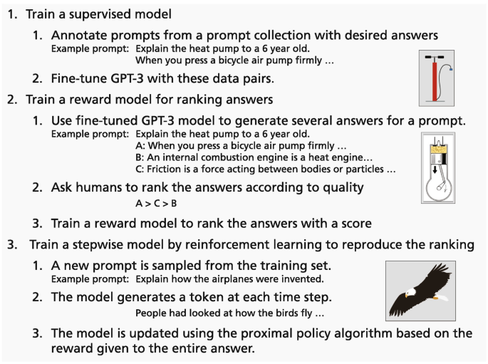

  

  InstructGPT is trained in three steps [151, p. 3]. First GPT-3 is fine-tuned on instructions and the corresponding completions. Then a reward model is generated by optimizing the selection of a completion for an instruction. Finally, a policy is trained to generate token by token of the answer with maximal reward. Credits for image parts in Table A.1

• 2. Pairs of trajectories (σ^[1], σ^[2]) from the {τ¹, …, τⁱ} are selected and submitted to a human for comparison.

• 3. The parameters u of the reward function $\hat {r}({\boldsymbol {y}},{\boldsymbol {x}};\boldsymbol {u})$ are optimized to correspond to the comparisons collected from the human up to now.

For a set of 33k instructions, a reward model$\hat {r}({\boldsymbol {y}},{\boldsymbol {x}};\boldsymbol {u})$ was built with 6B parameters, where x is the instruction and y a completion [198]. It selects the best completion from a small set of proposed completions. Proximal policy optimization (PPO) was used as reinforcement model [151, p. 41]. To avoid catastrophic forgetting (Sect. 3.6.1), pre-training samples were mixed into fine-tuning.

The reward model was then applied to create a final model by another reinforcement learning step. During this process, InstructGPT generates a completion for an instruction. The reward model calculates a reward and the policy is updated to approximate the preferences encoded in the reward model. By mimicking human utterances, the model implicitly learns human intentions and preferences. This process is called alignment to human preferences and is extensively discussed by Askell et al. [5].

3.6.5.1 InstructGPT Results

The GPT-3 model with 175B parameters fined-tuned in a supervised way to the 13k instruction-completion examples was taken as the base model called SFT. The final completions were again scored by human raters [151]. The InstructGPT completions were preferred to the standard GPT-3 output in 85% of cases and to few-shot-GPT-3 in 71% of cases.

Specifically, raters found that InstructGPT attempts to follow the correct instruction in 92% of cases, compared to 85% for SFT and 75% for few-shot GPT-3 [151, p. 53]. In addition, InstructGPT follows explicit constraints in 50% of the cases, compared to 43% for SFT and 34% for SFT and 28% for few-shot GPT-3. Hallucinations were observed for 20% of the cases for InstructGPT compared to 16% for SFT and 50% for few-shot GPT-3. Finally, the raters found that the language use is appropriate for a customer assistant in 92% of the cases for InstructGPT, about 90% for SFT and about 85% for GPT-3 few-shot. InstructGPT was also evaluated on a few natural language benchmarks where it achieved very similar results to GPT-3 [151, p. 56].

It turned out that InstructGPT is able to generalize to unseen labeler preferences. Thus, InstructGPT does not simply adapt to the preferences of a few training labelers. In addition, InstructGPT produces slightly less toxic language than standard GPT-3. However, InstructGPT still makes simple mistakes, e.g., given an instruction with a false premise, the model sometimes incorrectly assumes the premise is true. Note that the results depend on the subjective preferences of the labelers.

Comparisons between alternatives are not necessarily the most effective approach to generate an improvement signal. For example, one could ask labelers to edit model responses to make them better, or generate critiques of model responses in natural language. There is also a vast space of options for designing interfaces for labelers to provide feedback to language models; this is an interesting human-computer interaction problem. The authors note that the cost of aligning GPT-3 to human preferences described above is just 1.6% of the cost spent to train GPT-3. Therefore, it seems to make sense to put more effort into alignment than into the mere enlargement of the models.

The results show that the InstructGPT techniques potentially make language models more helpful, truthful, and harmless. In a way InstructGPT works like an intelligent assistant for speech generation and information provision. However, the model is currently not fit for use in safety-critical applications, because failures cannot be ruled out. What is still missing is a comprehensive evaluation similar to Gopher or PaLM (Sect. 3.1.2) that shows the real utility of this approach. It can be expected that the combination of this approach with retrieval techniques as used for WebGPT (Sect. 6.2.3) and Retro (Sect. 6.2.3) will increase the performance, reliability, and correctness of InstructGPT.

3.6.5.2 Instruction Tuning with FLAN

FLAN [227] uses instruction tuning to improve the ability of the language model to respond to natural language prompts. The language model has to learn through supervision to perform tasks described by prompts, and to follow instructions, even for unfamiliar tasks (Fig. 3.24). The authors group 62 publicly available NLP datasets into twelve task clusters, e.g. “sentiment” “natural language inference”, “summarization”, etc. For each of the datasets they compose ten templates describing the task in natural language. Then an existing language model is fine-tuned to provide better answers to the prompts.

Fig. 3.24

FLAN instruction tuning fine-tunes a pre-trained language models on a set of tasks with instructions of ten different templates (left). The trained model can be applied to unseen tasks by formulating prompts according to these templates (right). Image adapted from [227, p. 1] with kind permission of the authors

The approach was applied to a LaMDA-PT language model with 137B parameters using retrieval and filters (Sect. 6.6.3). For 18 NLI tasks the FLAN model was compared to LaMDA-PT 137B, GPT-3 175B, and GLaM 64B. In 14 of 18 cases FLAN substantially improved the performance of its unmodified counterpart and achieved better results than the competitors, while in 4 cases it was surpassed by GLaM [227]. FLAN even outperforms few-shot GPT-3 by a large margin on a number of tasks.

3.6.6 Generating Labeled Data by Foundation Models

The performance of GPT-3 and other Foundation Models in few-shot learning enables the generation of new high-quality training data for other models. By Unsupervised Data Generation (UDG) the creation of fine-tuning data for models of downstream tasks is possible that would otherwise be produced by manual human annotation. This approach is similar to Sect. 4.2.3.

The idea for data generation is to utilize the language model to learn the input-label relation based on the task description and a few sample input-label pairs [225]. Instead of generating and predicting a label for a classification task the language model has to create the input text using the output class and a task description as input. For a classification task like product reviews on Amazon, the approach is able to produce 10k new examples for each class, covering a much larger spectrum as the currently available labeled data. It turns out that up to 32 few-shot examples still increase the quality of the generated training data. Examples are shown in Fig. 3.25. The authors use an additional module to filter out noisy examples. In this approach, a given training example is removed if the trained classifier does not match its label with high probability.

Fig. 3.25

New data can be generated by GPT-3 and other Foundation Models using the few-shot UDG strategy. Here the prompts for two examples, Amazon reviews and Copa common sense reasoning, and the generated answers are shown [225]

The T5-XXL encoder-decoder model fine-tuned on SuperGLUE data enhanced with UDG data is able to improve the overall accuracy on the SuperGLUE task for natural language understanding to 90.4% and is even able to beat DeBERTa with 90.3%. Moreover, the approach achieves very high performance scores on a list of text classification and sentiment analysis tasks [225].

3.6.7 Summary

When pre-training Foundation Models on a big text collection and subsequent supervised fine-tuning on a small labeled dataset, PLMs achieved unprecedented performance on many NLP tasks. Fine-tuning has been shown to change model parameters only slightly and, in general, no catastrophic forgetting occurs. Usually, no overfitting is observed if fine-tuning is stopped after a few epochs. If necessary, there are some approaches to avoid overfitting.

Fine-tuning can be performed in different ways. It has been suggested to use an intermediate fine-tuning with a more related dataset before the final fine-tuning on the small dataset takes place. The results of such approaches have been mixed. Also, simultaneous fine-tuning to several tasks is possible. In some cases, it could improve performance. As an alternative, there are strategies to accelerate fine-tuning by meta-learning. To avoid that the full model is changed adapter layers can be defined, and only their parameters are adapted. This can drastically reduce the number of trainable parameters and nevertheless lead to good performance on the fine-tuning tasks. Finally, fine-tuning APIs have been recently provided for proprietary models like GPT-3.

Foundation Models like GPT-3 and PaLM can be instructed by prompts to solve specific tasks without training. A large number of different prompts has been collected to order the model to complete a task. InstructGPT is a new version of GPT-3 that directly takes instructions and provides the answers for a large spectrum of tasks. The model was customized to carry out the instructions by adapting to user judgments through reinforcement learning. Instruction tuning is a variant, where a Foundation Model is fine-tuned to provide improved answers to instructions for a number of tasks. It turns out that afterwards the model generates better answers even for unseen tasks.

Finally, big language models may be employed to generate high-quality training data for fine-tuning. Again, the few-shot learning technique is used to generate input texts for specific learning tasks. In this way, the scarce training data can be expanded and better fine-tuning results can be achieved.

References

O. Agarwal, H. Ge, S. Shakeri, and R. Al-Rfou. “Knowledge Graph Based Synthetic Corpus Generation for Knowledge-Enhanced Language Model Pre-training”. Mar. 13, 2021. arXiv: 2010.12688.
A. Aghajanyan, A. Shrivastava, A. Gupta, N. Goyal, L. Zettlemoyer, and S. Gupta. “Better Fine-Tuning by Reducing Representational Collapse”. Aug. 6, 2020. arXiv: 2008.03156.
J. Ainslie, S. Ontanon, C. Alberti, P. Pham, A. Ravula, and S. Sanghai. “ETC: Encoding Long and Structured Data in Transformers”. 2020. arXiv: 2004.08483.
A. Alvi. Using DeepSpeed and Megatron to Train Megatron-Turing NLG 530B, the World fs Largest and Most Powerful Generative Language Model. Microsoft Research. Oct. 11, 2021. url: https://www.microsoft.com/en-us/research/blog/using-deepspeed-andmegatron-to-train-megatron-turing-nlg-530b-the-worlds-largest-and-most-powerful-generative-language-model/ (visited on 11/12/2021).
A. Askell et al. “A General Language Assistant as a Laboratory for Alignment”. Dec. 9, 2021. arXiv: 2112.00861 [cs].
T. Bansal, R. Jha, T. Munkhdalai, and A. McCallum. “Self-Supervised Meta-Learning for Few-Shot Natural Language Classification Tasks”. 2020. arXiv: 2009.08445.
Y. Bansal, G. Kaplun, and B. Barak. “For Self-Supervised Learning, Rationality Implies Generalization, Provably”. 2020. arXiv: 2010.08508.
H. Bao et al. “Unilmv2: Pseudo-masked Language Models for Unified Language Model Pre-Training”. In: Int. Conf. Mach. Learn. PMLR, 2020, pp. 642–652.
A. Bapna et al. Building Machine Translation Systems for the Next Thousand Languages. May 16, 2022. arXiv: 2205.03983 [cs].
I. Beltagy, M. E. Peters, and A. Cohan. “Longformer: The Long-Document Transformer”. 2020. arXiv: 2004.05150.
benchmark. GLUE Benchmark. Aug. 5, 2021. url: https://gluebenchmark.com/ (visited on 08/05/2021).
Y. Bengio, A. Courville, and P. Vincent. “Representation Learning: A Review and New Perspectives”. In: IEEE Trans. Pattern Anal. Mach. Intell. 35.8 (2013), pp. 1798–1828.
J. Berant, A. Chou, R. Frostig, and P. Liang. “Semantic Parsing on Freebase from Question-Answer Pairs”. In: Proc. 2013 Conf. Empir. Methods Nat. Lang. Process. EMNLP 2013. Seattle, Washington, USA: Association for Computational Linguistics, Oct. 2013, pp. 1533–1544. url: https://aclanthology.org/D13-1160 (visited on 12/14/2021).
M. Bevilacqua and R. Navigli. “Breaking through the 80% Glass Ceiling: Raising the State of the Art in Word Sense Disambiguation by Incorporating Knowledge Graph Information”. In: Proc Assoc. Comput. Linguist. 2020, pp. 2854–2864.
C. Bizer, J. Lehmann, G. Kobilarov, S. Auer, C. Becker, R. Cyganiak, and S. Hellmann. “DBpedia-A Crystallization Point for the Web of Data”. In: J. Web Semant. 7.3 (2009), pp. 154–165.
S. Black, G. Leo, P. Wang, C. Leahy, and S. Biderman. GPT-Neo: Large Scale Autoregressive Language Modeling with Mesh-Tensorflow. Zenodo, Mar. 21, 2021. https://doi.org/10.5281/zenodo.5297715.
O. Bojar et al. “Findings of the 2014 Workshop on Statistical Machine Translation”. In: Proc. Ninth Workshop Stat. Mach. Transl. 2014, pp. 12–58.
K. Bollacker, C. Evans, P. Paritosh, T. Sturge, and J. Taylor. “Freebase: A Collaboratively Created Graph Database for Structuring Human Knowledge”. In: Proc. 2008 ACM SIGMOD Int. Conf. Manag. Data. 2008, pp. 1247–1250.
R. Bommasani et al. “On the Opportunities and Risks of Foundation Models”. 2021. arXiv: 2108.07258.
A. Bordes, N. Usunier, A. Garcia-Duran, J. Weston, and O. Yakhnenko. “Translating Embeddings for Modeling Multi-Relational Data”. In: Adv. Neural Inf. Process. Syst. 26 (2013), pp. 2787–2795.
S. Borgeaud et al. “Improving Language Models by Retrieving from Trillions of Tokens”. Dec. 8, 2021. arXiv: 2112.04426 [cs].
A. Borzunov et al. Petals: Collaborative Inference and Fine-tuning of Large Models. Sept. 2, 2022. https://doi.org/10.48550/2209.01188. arXiv: 2209.01188 [cs].
G. Branwen. “GPT-3 Creative Fiction”. In: (June 19, 2020). url: https://www.gwern.net/GPT-3 (visited on 11/14/2021).
S. Brin and L. Page. “The Anatomy of a Large-Scale Hypertextual Web Search Engine”. In: Comput. Netw. ISDN Syst. 30.1-7 (1998), pp. 107–117.
T. B. Brown et al. “Language Models Are Few-Shot Learners”. 2020. arXiv: 2005.14165.
J. Casper. What Is This Fork of Megatron-LM and Megatron-DeepSpeed. BigScience Workshop, Oct. 25, 2022. url: https://github.com/bigscience-workshop/Megatron-DeepSpeed (visited on 10/25/2022).
D. Chen. Openqa-Tutorial Danqi/Acl2020. July 5, 2020. url: https://github.com/danqi/acl2020-openqa-tutorial (visited on 02/24/2021).
Q. Chen, C. Shui, and M. Marchand. “Generalization Bounds For Meta-Learning: An Information-Theoretic Analysis”. In: Adv. Neural Inf. Process. Syst. 34 (2021).
T. Chen, J. Frankle, S. Chang, S. Liu, Y. Zhang, Z. Wang, and M. Carbin. “The Lottery Ticket Hypothesis for Pre-Trained Bert Networks”. 2020. arXiv: 2007.12223.
W. Chen, Y. Su, X. Yan, and W. Y. Wang. “KGPT: Knowledge-Grounded Pre-Training for Data-to-Text Generation”. 2020. arXiv: 2010.02307.
Z. Chi, L. Dong, S. Ma, S. H. X.-L. Mao, H. Huang, and F. Wei. “mT6: Multilingual Pretrained Text-to-Text Transformer with Translation Pairs”. 2021. arXiv: 2104.08692.
Z. Chi, L. Dong, F. Wei, W. Wang, X.-L. Mao, and H. Huang. “Cross-Lingual Natural Language Generation via Pre-Training.” In: AAAI. 2020, pp. 7570–7577.
R. Child, S. Gray, A. Radford, and I. Sutskever. “Generating Long Sequences with Sparse Transformers”. 2019. arXiv: 1904.10509.
K. Choromanski et al. “Rethinking Attention with Performers”. 2020. arXiv: 2009.14794.
A. Chowdhery et al. “PaLM: Scaling Language Modeling with Pathways”. Apr. 5, 2022. arXiv: 2204.02311 [cs].
P. F. Christiano, J. Leike, T. Brown, M. Martic, S. Legg, and D. Amodei. “Deep Reinforcement Learning from Human Preferences”. In: Adv. Neural Inf. Process. Syst. 30 (2017).
H. W. Chung, T. Févry, H. Tsai, M. Johnson, and S. Ruder. “Rethinking Embedding Coupling in Pre-Trained Language Models”. 2020. arXiv: 2010.12821.
A. Clark et al. “Unified Scaling Laws for Routed Language Models”. Feb. 9, 2022. arXiv: 2202.01169 [cs].
K. Clark, M.-T. Luong, Q. V. Le, and C. D. Manning. “Electra: Pre-training Text Encoders as Discriminators Rather than Generators”. 2020. arXiv: 2003.10555.
A. Conneau, G. Lample, R. Rinott, A. Williams, S. R. Bowman, H. Schwenk, and V. Stoyanov. “XNLI: Evaluating Cross-lingual Sentence Representations”. Sept. 13, 2018. arXiv: 1809.05053.
A. Conneau et al. “Unsupervised Cross-Lingual Representation Learning at Scale”. Apr. 8, 2020. arXiv: 1911.02116.
A. D’Amour. How Underspecification Presents Challenges for Machine Learning. Google AI Blog. Oct. 18, 2021. url: http://ai.googleblog.com/2021/10/how-underspecificationpresents.html (visited on 10/25/2021).
Y. Dai, S. Wang, N. N. Xiong, and W. Guo. “A Survey on Knowledge Graph Embedding: Approaches, Applications and Benchmarks”. In: Electronics 9.5 (2020), p. 750.
Z. Dai, Z. Yang, Y. Yang, W. W. Cohen, J. Carbonell, Q. V. Le, and R. Salakhutdinov. “Transformer-XL: Language Modeling with Longer-Term Dependency, 2019”. In: URL Httpsopenreview Netforum. 2019.
T. Dash, S. Chitlangia, A. Ahuja, and A. Srinivasan. “Incorporating Domain Knowledge into Deep Neural Networks”. 2021. arXiv: 2103.00180.
L. de Alwis, A. Dissanayake, M. Pallewatte, K. Silva, and U. Thayasivam. “Survey on Semantic Table Interpretation”. In: (July 13, 2018). url: http://semantic-web-journal.org/system/files/swj1946.pdf.
X. Deng, H. Sun, A. Lees, Y. Wu, and C. Yu. “Turl: Table Understanding through Representation Learning”. Dec. 3, 2020. arXiv: 2006.14806.
J. Devlin. mBERT - Multilingual BERT. GitHub. 2019. url: https://github.com/googleresearch/bert/blob/master/multilingual.md (visited on 02/21/2021).
J. Devlin, M.-W. Chang, K. Lee, and K. Toutanova. “Bert: Pre-training of Deep Bidirectional Transformers for Language Understanding”. 2018. arXiv: 1810.04805.
T. Dozat and C. D. Manning. “Deep Biaffine Attention for Neural Dependency Parsing”. 2016. arXiv: 1611.01734.
N. Du et al. “GLaM: Efficient Scaling of Language Models with Mixture-of-Experts”. Dec. 13, 2021. arXiv: 2112.06905 [cs].
S. S. Du, W. Hu, S. M. Kakade, J. D. Lee, and Q. Lei. “Few-Shot Learning via Learning the Representation, Provably”. 2020. arXiv: 2002.09434.
Z. Du. GLM. THUDM, Dec. 14, 2021. url: https://github.com/THUDM/GLM (visited on 12/17/2021).
Z. Du, Y. Qian, X. Liu, M. Ding, J. Qiu, Z. Yang, and J. Tang. “All NLP Tasks Are Generation Tasks: A General Pretraining Framework”. Mar. 18, 2021. arXiv: 2103.10360 [cs].
Z. Du, Y. Qian, X. Liu, M. Ding, J. Qiu, Z. Yang, and J. Tang. GLM: General Language Model Pretraining with Autoregressive Blank Infilling. Nov. 1, 2021. url: https://aclanthology.org/2022.acl-long.26/ (visited on 12/17/2021).
W. Fedus, B. Zoph, and N. Shazeer. “Switch Transformers: Scaling to Trillion Parameter Models with Simple and Efficient Sparsity”. 2021. arXiv: 2101.03961.
F. Feng, Y. Yang, D. Cer, N. Arivazhagan, and W. Wang. “Language-Agnostic BERT Sentence Embedding”. July 3, 2020. arXiv: 2007.01852 [cs].
C. Finn, P. Abbeel, and S. Levine. “Model-Agnostic Meta-Learning for Fast Adaptation of Deep Networks”. In: Int. Conf. Mach. Learn. PMLR, 2017, pp. 1126–1135.
Q. Fournier, G. M. Caron, and D. Aloise. “A Practical Survey on Faster and Lighter Transformers”. Mar. 26, 2021. arXiv: 2103.14636 [cs].
P. Ganesh et al. “Compressing Large-Scale Transformer-Based Models: A Case Study on Bert”. 2020. arXiv: 2002.11985.
L. Gao et al. “The Pile: An 800GB Dataset of Diverse Text for Language Modeling”. 2020. arXiv: 2101.00027.
T. Gao, A. Fisch, and D. Chen. “Making Pre-Trained Language Models Better Few-Shot Learners”. 2020. arXiv: 2012.15723.
H. Gong, Y. Sun, X. Feng, B. Qin, W. Bi, X. Liu, and T. Liu. “Tablegpt: Few-shot Tableto-Text Generation with Table Structure Reconstruction and Content Matching”. In: Proc. 28th Int. Conf. Comput. Linguist. 2020, pp. 1978–1988.
M. A. Gordon, K. Duh, and N. Andrews. “Compressing BERT: Studying the Effects of Weight Pruning on Transfer Learning”. 2020. arXiv: 2002.08307.
J. Gou, B. Yu, S. Maybank, and D. Tao. “Knowledge Distillation: A Survey”. Jan. 26, 2021. arXiv: 2006.05525.
N. Goyal, J. Du, M. Ott, G. Anantharaman, and A. Conneau. “Larger-Scale Transformers for Multilingual Masked Language Modeling”. 2021. arXiv: 2105.00572.
A. Grover and J. Leskovec. “Node2vec: Scalable Feature Learning for Networks”. In: Proc. 22nd ACM SIGKDD Int. Conf. Knowl. Discov. Data Min. 2016, pp. 855–864.
A. Gu, K. Goel, and C. Ré. “Efficiently Modeling Long Sequences with Structured State Spaces”. 2021. arXiv: 2111.00396.
A. Gu, K. Goel, and C. Ré. The Annotated S4. 2021. url: https://srush.github.io/annotateds4/ (visited on 04/05/2022).
A. Gupta. “Diagonal State Spaces Are as Effective as Structured State Spaces”. 2022. arXiv: 2203.14343.
S. Gururangan, A. Marasović, S. Swayamdipta, K. Lo, I. Beltagy, D. Downey, and N. A. Smith. “Don’t Stop Pretraining: Adapt Language Models to Domains and Tasks”. 2020. arXiv: 2004.10964.
K. Guu, K. Lee, Z. Tung, P. Pasupat, and M.-W. Chang. “Realm: Retrieval-augmented Language Model Pre-Training”. 2020. arXiv: 2002.08909.
C. Hawthorne et al. “General-Purpose, Long-Context Autoregressive Modeling with Perceiver AR”. 2022. arXiv: 2202.07765.
J. He, J. Qiu, A. Zeng, Z. Yang, J. Zhai, and J. Tang. “FastMoE: A Fast Mixture-of-Expert Training System”. Mar. 24, 2021. arXiv: 2103.13262 [cs].
P. He, J. Gao, and W. Chen. “Debertav3: Improving Deberta Using Electra-Style Pre-Training with Gradient-Disentangled Embedding Sharing”. 2021. arXiv: 2111.09543.
P. He, X. Liu, J. Gao, and W. Chen. “DeBERTa: Decoding-enhanced BERT with Disentangled Attention”. Jan. 11, 2021. arXiv: 2006.03654.
W. D. Heaven. This Know-It-All AI Learns by Reading the Entire Web Nonstop. MIT Technology Review. Sept. 4, 2020. url: https://www.technologyreview.com/2020/09/04/1008156/knowledge-graph-ai-reads-web-machine-learning-natural-language-processing/ (visited on 12/01/2021).
K. M. Hermann, T. Kocisky, E. Grefenstette, L. Espeholt, W. Kay, M. Suleyman, and P. Blunsom. “Teaching Machines to Read and Comprehend”. 2015. arXiv: 1506.03340.
A. Hern. “TechScape: AI’s Dark Arts Come into Their Own”. In: The Guardian. Technology (Sept. 21, 2022). issn: 0261-3077. url: https://www.theguardian.com/technology/2022/sep/21/ais-dark-arts-come-into-their-own (visited on 10/01/2022).
D. Hernandez, J. Kaplan, T. Henighan, and S. McCandlish. “Scaling Laws for Transfer”. Feb. 1, 2021. arXiv: 2102.01293 [cs].
J. Herzig, P. K. Nowak, T. Müller, F. Piccinno, and J. M. Eisenschlos. “Tapas: Weakly Supervised Table Parsing via Pre-Training”. 2020. arXiv: 2004.02349.
G. Hinton, O. Vinyals, and J. Dean. “Distilling the Knowledge in a Neural Network”. 2015. arXiv: 1503.02531.
J. Hoffmann et al. “Training Compute-Optimal Large Language Models”. 2022. arXiv: 2203.15556.
N. Houlsby et al. “Parameter-Efficient Transfer Learning for NLP”. In: Int. Conf. Mach. Learn. PMLR, 2019, pp. 2790–2799.
E. J. Hu, Y. Shen, P. Wallis, Z. Allen-Zhu, Y. Li, S. Wang, and W. Chen. “LoRA: Low- Rank Adaptation of Large Language Models”. 2021. arXiv: 2106.09685.
J. Hu, S. Ruder, A. Siddhant, G. Neubig, O. Firat, and M. Johnson. “Xtreme: A Massively Multilingual Multi-Task Benchmark for Evaluating Cross-Lingual Generalisation”. In: Int. Conf. Mach. Learn. PMLR, 2020, pp. 4411–4421.
Z. Hu, Y. Dong, K. Wang, K.-W. Chang, and Y. Sun. “Gpt-Gnn: Generative Pre-Training of Graph Neural Networks”. In: Proc. 26th ACM SIGKDD Int. Conf. Knowl. Discov. Data Min. 2020, pp. 1857–1867.
H. Huang, Y. Liang, N. Duan, M. Gong, L. Shou, D. Jiang, and M. Zhou. “Unicoder: A Universal Language Encoder by Pre-Training with Multiple Cross-Lingual Tasks”. 2019. arXiv: 1909.00964.
A. Iyer. GPT-3’s Free Alternative GPT-Neo Is Something to Be Excited About. Venture- Beat. May 15, 2021. url: https://venturebeat.com/2021/05/15/gpt-3s-free-alternative-gptneo-is-something-to-be-excited-about/ (visited on 01/03/2022).
M. Iyyer, W.-t. Yih, and M.-W. Chang. “Search-Based Neural Structured Learning for Sequential Question Answering”. In: Proc. 55th Annu. Meet. Assoc. Comput. Linguist. Vol. 1 Long Pap. 2017, pp. 1821–1831.
G. Izacard and E. Grave. “Leveraging Passage Retrieval with Generative Models for Open Domain Question Answering”. In: Proc. 16th Conf. Eur. Chapter Assoc. Comput. Linguist. Main Vol. EACL 2021. Online: Association for Computational Linguistics, Apr. 1, 2021, pp. 874–880. url: https://www.aclweb.org/anthology/2021.eacl-main.74 (visited on 06/16/2021).
A. Jaegle, F. Gimeno, A. Brock, A. Zisserman, O. Vinyals, and J. Carreira. “Perceiver: General Perception with Iterative Attention”. June 22, 2021. arXiv: 2103.03206 [cs, eess].
A. Jaegle et al. “Perceiver IO: A General Architecture for Structured Inputs & Outputs”. Aug. 2, 2021. arXiv: 2107.14795.
S. Ji, S. Pan, E. Cambria, P. Marttinen, and S. Y. Philip. “A Survey on Knowledge Graphs: Representation, Acquisition, and Applications”. In: IEEE Trans. Neural Netw. Learn. Syst. (2021).
H. Jiang, P. He, W. Chen, X. Liu, J. Gao, and T. Zhao. “SMART: Robust and Efficient Fine-Tuning for Pre-trained Natural Language Models through Principled Regularized Optimization”. In: Proc. 58th Annu. Meet. Assoc. Comput. Linguist. ACL 2020. Online: Association for Computational Linguistics, July 2020, pp. 2177–2190. https://doi.org/10.18653/v1/2020.acl-main.197.
Z. Jiang, F. F. Xu, J. Araki, and G. Neubig. “How Can We Know What Language Models Know?” In: Trans. Assoc. Comput. Linguist. 8 (2020), pp. 423–438.
X. Jiao et al. “Tinybert: Distilling Bert for Natural Language Understanding”. 2019. arXiv: 1909.10351.
M. Joshi, D. Chen, Y. Liu, D. S. Weld, L. Zettlemoyer, and O. Levy. “Spanbert: Improving Pre-Training by Representing and Predicting Spans”. In: Trans. Assoc. Comput. Linguist. 8 (2020), pp. 64–77.
M. Joshi, E. Choi, D. S. Weld, and L. Zettlemoyer. “Triviaqa: A Large Scale Distantly Supervised Challenge Dataset for Reading Comprehension”. 2017. arXiv: 1705.03551.
D. Jurafsky and J. H. Martin. Speech and Language ProcessingAn Introduction to Natural Language Processing,Computational Linguistics, and Speech Recognition. 3rd Draft. Jan. 12, 2022.
R. E. Kalman. “A New Approach to Linear Filtering and Prediction Problems”. In: (1960).
J. Kaplan et al. “Scaling Laws for Neural Language Models”. 2020. arXiv: 2001.08361.
V. Karpukhin, B. Oğuz, S. Min, L. Wu, S. Edunov, D. Chen, and W.-t. Yih. “Dense Passage Retrieval for Open-Domain Question Answering”. 2020. arXiv: 2004.04906.
K. Karthikeyan, Z. Wang, S. Mayhew, and D. Roth. “Cross-Lingual Ability of Multilingual BERT: An Empirical Study”. Feb. 15, 2020. arXiv: 1912.07840.
A. Katharopoulos, A. Vyas, N. Pappas, and F. Fleuret. “Transformers Are Rnns: Fast Autoregressive Transformers with Linear Attention”. In: Int. Conf. Mach. Learn. PMLR, 2020, pp. 5156–5165.
P. Kharya and A. Alvi. Using DeepSpeed and Megatron to Train Megatron-Turing NLG 530B, the World’s Largest and Most Powerful Generative Language Model. NVIDIA Developer Blog. Oct. 11, 2021. url: https://developer.nvidia.com/blog/using-deepspeed-andmegatron-to-train-megatron-turing-nlg-530b-the-worlds-largest-and-most-powerful-generativelanguage-model/ (visited on 01/08/2022).
T. N. Kipf and M. Welling. “Semi-Supervised Classification with Graph Convolutional Networks”. 2016. arXiv: 1609.02907.
N. Kitaev, L. Kaiser, and A. Levskaya. “Reformer: The Efficient Transformer”. 2020. arXiv: 2001.04451.
T. Kwiatkowski et al. “Natural Questions: A Benchmark for Question Answering Research”. In: Trans. Assoc. Comput. Linguist. 7 (2019), pp. 453–466.
G. Lai, Q. Xie, H. Liu, Y. Yang, and E. Hovy. “Race: Large-scale Reading Comprehension Dataset from Examinations”. 2017. arXiv: 1704.04683.
G. Lample and A. Conneau. “Cross-Lingual Language Model Pretraining”. 2019. arXiv: 1901.07291.
G. Lample, A. Sablayrolles, M. Ranzato, L. Denoyer, and H. Jégou. “Large Memory Layers with Product Keys”. 2019. arXiv: 1907.05242.
Z. Lan, M. Chen, S. Goodman, K. Gimpel, P. Sharma, and R. Soricut. “Albert: A Lite BERT for Self-Supervised Learning of Language Representations”. 2020. arXiv: 1909.11942.
J. Lee, M. Sung, J. Kang, and D. Chen. “Learning Dense Representations of Phrases at Scale”. Jan. 2, 2021. arXiv: 2012.12624.
O. Lehmberg, D. Ritze, R. Meusel, and C. Bizer. “A Large Public Corpus of Web Tables Containing Time and Context Metadata”. In: Proc. 25th Int. Conf. Companion World Wide Web. 2016, pp. 75–76.
D. Lepikhin et al. “Gshard: Scaling Giant Models with Conditional Computation and Automatic Sharding”. 2020. arXiv: 2006.16668.
B. Lester, R. Al-Rfou, and N. Constant. “The Power of Scale for Parameter-Efficient Prompt Tuning”. 2021. arXiv: 2104.08691.
M. Lewis, M. Ghazvininejad, G. Ghosh, A. Aghajanyan, S. Wang, and L. Zettlemoyer. “Pre-Training via Paraphrasing”. 2020. arXiv: 2006.15020.
M. Lewis et al. “Bart: Denoising Sequence-to-Sequence Pre-Training for Natural Language Generation, Translation, and Comprehension”. 2020. arXiv: 1910.13461.
P. Li et al. “An Effective Self-Supervised Framework for Learning Expressive Molecular Global Representations to Drug Discovery”. In: Brief Bioinform 22.6 (Nov. 5, 2021), bbab109. issn: 1477-4054. https://doi.org/10.1093/bib/bbab109. pmid: 33940598.
X. L. Li and P. Liang. “Prefix-Tuning: Optimizing Continuous Prompts for Generation”. 2021. arXiv: 2101.00190.
O. Lieber, O. Sharir, B. Lentz, and Y. Shoham. “Jurassic-1: Technical Details and Evaluation”. In: (2021), p. 9. url: https://uploads-ssl.webflow.com/60fd4503684b466578c0d307/61138924626a6981ee09caf6_jurassic_tech_paper.pdf.
R. Lim, M. Wu, and L. Miller. Customizing GPT-3 for Your Application. OpenAI. Dec. 14, 2021. url: https://openai.com/blog/customized-gpt-3/ (visited on 02/16/2022).
X. V. Lin, R. Socher, and C. Xiong. “Bridging Textual and Tabular Data for Cross-Domain Text-to-Sql Semantic Parsing”. 2020. arXiv: 2012.12627.
P. Liu, W. Yuan, J. Fu, Z. Jiang, H. Hayashi, and G. Neubig. “Pre-Train, Prompt, and Predict: A Systematic Survey of Prompting Methods in Natural Language Processing”. 2021. arXiv: 2107.13586.
Y. Liu et al. “Multilingual Denoising Pre-Training for Neural Machine Translation”. 2020. arXiv: 2001.08210.
Y. Liu et al. “Roberta: A Robustly Optimized Bert Pretraining Approach”. 2019. arXiv: 1907.11692.
Y. Liu, S. Pan, M. Jin, C. Zhou, F. Xia, and P. S. Yu. “Graph Self-Supervised Learning: A Survey”. 2021. arXiv: 2103.00111.
F. Locatello, S. Bauer, M. Lucic, G. Raetsch, S. Gelly, B. Schölkopf, and O. Bachem. “Challenging Common Assumptions in the Unsupervised Learning of Disentangled Representations”. In: Int. Conf. Mach. Learn. PMLR, 2019, pp. 4114–4124.
A. Maas, R. E. Daly, P. T. Pham, D. Huang, A. Y. Ng, and C. Potts. “Learning Word Vectors for Sentiment Analysis”. In: Proc. 49th Annu. Meet. Assoc. Comput. Linguist. Hum. Lang. Technol. 2011, pp. 142–150.
D. Mahajan et al. “Identification of Semantically Similar Sentences in Clinical Notes: Iterative Intermediate Training Using Multi-Task Learning”. In: JMIR Med. Inform. 8.11 (2020), e22508.
S. McCandlish, J. Kaplan, D. Amodei, and O. D. Team. “An Empirical Model of Large-Batch Training”. 2018. arXiv: 1812.06162.
A. Merchant, E. Rahimtoroghi, E. Pavlick, and I. Tenney. “What Happens To BERT Embeddings During Fine-tuning?” Apr. 29, 2020. arXiv: 2004.14448.
S. Merity, C. Xiong, J. Bradbury, and R. Socher. “Pointer Sentinel Mixture Models”. 2016. arXiv: 1609.07843.
T. Mikolov, K. Chen, G. Corrado, and J. Dean. “Efficient Estimation of Word Representations in Vector Space”. 2013. arXiv: 1301.3781.
T. Mikolov and G. Zweig. “Context Dependent Recurrent Neural Network Language Model”. In: 2012 IEEE Spok. Lang. Technol. Workshop SLT. IEEE, 2012, pp. 234–239.
G. A. Miller. “WordNet: A Lexical Database for English”. In: Commun. ACM 38.11 (1995), pp. 39–41.
S. Mishra, D. Khashabi, C. Baral, and H. Hajishirzi. “Cross-Task Generalization via Natural Language Crowdsourcing Instructions”. Mar. 14, 2022. arXiv: 2104.08773 [cs].
M. Mitchell. BigScience Large Open-science Open-access Multilingual Language Model. July 6, 2022. url: https://huggingface.co/bigscience/bloom (visited on 10/25/2022).
M. Mosbach, M. Andriushchenko, and D. Klakow. “On the Stability of Fine-Tuning Bert: Misconceptions, Explanations, and Strong Baselines”. Mar. 25, 2021. arXiv: 2006.04884.
A. Mulyar, O. Uzuner, and B. McInnes. “MT-clinical BERT: Scaling Clinical Information Extraction with Multitask Learning”. In: J. Am. Med. Inform. Assoc. 28.10 (2021), pp. 2108–2115.
S. Narang et al. “Do Transformer Modifications Transfer Across Implementations and Applications?” Sept. 10, 2021. arXiv: 2102.11972 [cs].
S. Narayan, S. B. Cohen, and M. Lapata. “Don’t Give Me the Details, Just the Summary! Topic-Aware Convolutional Neural Networks for Extreme Summarization”. In: Proc. 2018 Conf. Empir. Methods Nat. Lang. Process. EMNLP 2018. Brussels, Belgium: Association for Computational Linguistics, Oct. 2018, pp. 1797–1807. https://doi.org/10.18653/v1/D18-1206.
M. Nayyeri, S. Vahdati, C. Aykul, and J. Lehmann. “5* Knowledge Graph Embeddings with Projective Transformations”. 2020. arXiv: 2006.04986.
M. Nickel, V. Tresp, and H.-P. Kriegel. “A Three-Way Model for Collective Learning on Multi-Relational Data”. In: Icml. 2011.
Y. Nie, A. Williams, E. Dinan, M. Bansal, J. Weston, and D. Kiela. “Adversarial Nli: A New Benchmark for Natural Language Understanding”. 2019. arXiv: 1910.14599.
S. J. Nowlan and G. E. Hinton. “Evaluation of Adaptive Mixtures of Competing Experts.” In: NIPS. Vol. 3. 1990, pp. 774–780.
A. van den Oord et al. “Wavenet: A Generative Model for Raw Audio”. 2016. arXiv: 1609.03499.
OpenAi. OpenAI API. 2021. url: https://beta.openai.com (visited on 11/14/2021).
OpenAi. Prompt Examples for GPT-3. Sept. 3, 2021. url: https://beta.openai.com/examples (visited on 09/03/2021).
L. Ouyang et al. “Training Language Models to Follow Instructions with Human Feedback”. Jan. 31, 2022. arXiv: 2203.02155.
G. Paass and J. Kindermann. “Bayesian Classification Trees with Overlapping Leaves Applied to Credit-Scoring”. In: Res. Dev. Knowl. Discov. Data Min. Ed. by X. Wu, R. Ko tagiri, and K. B. Korb. Lecture Notes in Computer Science. Berlin, Heidelberg: Springer, 1998, pp. 234–245. isbn: 978-3-540-69768-8. https://doi.org/10.1007/3-540-64383-4_20.
V. Pan. “Fast Approximate Computations with Cauchy Matrices and Polynomials”. In: Math. Comput. 86.308 (2017), pp. 2799–2826.
D. Paperno et al. “The LAMBADA Dataset: Word Prediction Requiring a Broad Discourse Context”. June 20, 2016. arXiv: 1606.06031 [cs].
P. Pasupat and P. Liang. “Compositional Semantic Parsing on Semi-Structured Tables”. 2015. arXiv: 1508.00305.
M. E. Peters, M. Neumann, M. Iyyer, M. Gardner, C. Clark, K. Lee, and L. Zettlemoyer. “Deep Contextualized Word Representations”. In: Proc. NAACL-HLT. 2018, pp. 2227–2237.
M. E. Peters, M. Neumann, R. L. Logan IV, R. Schwartz, V. Joshi, S. Singh, and N. A. Smith. “Knowledge Enhanced Contextual Word Representations”. 2019. arXiv: 1909.04164.
F. Petroni. LAMA: LAnguage Model Analysis. Meta Research, 2020. url: https://github.com/facebookresearch/LAMA (visited on 03/08/2022).
F. Petroni, T. Rocktäschel, P. Lewis, A. Bakhtin, Y. Wu, A. H. Miller, and S. Riedel. “Language Models as Knowledge Bases?” 2019. arXiv: 1909.01066.
J. Pfeiffer, I. Vulic̀, I. Gurevych, and S. Ruder. “Mad-x: An Adapter-Based Framework for Multi-Task Cross-Lingual Transfer”. 2020. arXiv: 2005.00052.
J. Pfeiffer et al. “Adapterhub: A Framework for Adapting Transformers”. 2020. arXiv: 2007.07779.
N. Poerner, U. Waltinger, and H. Schütze. “Bert Is Not a Knowledge Base (yet): Factual Knowledge vs. Name-Based Reasoning in Unsupervised Qa”. 2019. arXiv: 1911.03681.
C. Poth, J. Pfeiffer, A. Rücklé, and I. Gurevych. “What to Pre-Train on? Efficient Intermediate Task Selection”. 2021. arXiv: 2104.08247.
S. Pradhan, A. Moschitti, N. Xue, O. Uryupina, and Y. Zhang. “CoNLL-2012 Shared Task: Modeling Multilingual Unrestricted Coreference in OntoNotes”. In: Jt. Conf. EMNLP CoNLL-Shar. Task. 2012, pp. 1–40.
Y. Pruksachatkun et al. “Intermediate-Task Transfer Learning with Pretrained Models for Natural Language Understanding: When and Why Does It Work?” 2020. arXiv: 2005.00628.
X. Qiu, T. Sun, Y. Xu, Y. Shao, N. Dai, and X. Huang. “Pre-Trained Models for Natural Language Processing: A Survey”. In: Sci. China Technol. Sci. 63.10 (June 23, 2021), pp. 1872–1897. issn: 1674–7321, 1869–1900. https://doi.org/10.1007/s11431-020-1647-3. arXiv: 2003.08271.
A. Radford, J. Wu, R. Child, D. Luan, D. Amodei, and I. Sutskever. “Language Models Are Unsupervised Multitask Learners”. In: OpenAI blog 1.8 (2019), p. 9.
J. W. Rae et al. “Scaling Language Models: Methods, Analysis & Insights from Training Gopher”. In: ArXiv Prepr. ArXiv211211446 (Dec. 8, 2021), p. 118.
J. W. Rae, A. Potapenko, S. M. Jayakumar, and T. P. Lillicrap. “Compressive Transformers for Long-Range Sequence Modelling”. 2019. arXiv: 1911.05507.
C. Raffel et al. “Exploring the Limits of Transfer Learning with a Unified Text-to-Text Transformer”. In: J. Mach. Learn. Res. 21.140 (2020), pp. 1–67.
c. raffel. C4 — TensorFlow Datasets. TensorFlow. 2019. url: https://www.tensorflow.org/datasets/catalog/c4 (visited on 12/14/2021).
A. Raganato, Y. Scherrer, and J. Tiedemann. “Fixed Encoder Self-Attention Patterns in Transformer-Based Machine Translation”. 2020. arXiv: 2002.10260.
P. Rajpurkar, J. Zhang, K. Lopyrev, and P. Liang. “Squad: 100,000+ Questions for Machine Comprehension of Text”. 2016. arXiv: 1606.05250.
H. Ren, H. Dai, Z. Dai, M. Yang, J. Leskovec, D. Schuurmans, and B. Dai. “Combiner: Full Attention Transformer with Sparse Computation Cost”. In: Adv. Neural Inf. Process. Syst. 34 (2021).
J. Rodriguez. Five Key Facts Wu Dao 2.0: The Largest Transformer Model Ever Built. DataSeries. Sept. 21, 2021. url: https://medium.com/dataseries/five-key-facts-wu-dao-2-0-the-largest-transformer-model-ever-built-19316159796b (visited on 12/12/2021).
A. Rogers, O. Kovaleva, and A. Rumshisky. “A Primer in {Bertology}: What We Know about How {BERT} Works”. In: Trans. Assoc. Comput. Linguist. 8 (2021), pp. 842–866.
S. Roller, S. Sukhbaatar, A. Szlam, and J. Weston. “Hash Layers For Large Sparse Models”. 2021. arXiv: 2106.04426.
A. Romero. GPT-3 Scared You? Meet Wu Dao 2.0: A Monster of 1.75 Trillion Parameters. Medium. June 8, 2021. url: https://towardsdatascience.com/gpt-3-scared-you-meet-wu-dao-2-0-a-monster-of-1-75-trillion-parameters-832cd83db484 (visited on 07/29/2021).
C. Rosset. “Turing-Nlg: A 17-Billion-Parameter Language Model by Microsoft”. In: Microsoft Blog — 13.02 2020 (2019).
A. Roy, M. Saffar, A. Vaswani, and D. Grangier. “Efficient Content-Based Sparse Attention with Routing Transformers”. 2020. arXiv: 2003.05997.
A. Sabeti. GPT-3: An AI That’s Eerily Good at Writing Almost Anything. Arram Sabeti. July 9, 2020. url: https://arr.am/2020/07/09/gpt-3-an-ai-thats-eerily-good-at-writing-almostanything/ (visited on 09/04/2021).
K. Sakaguchi, R. Le Bras, C. Bhagavatula, and Y. Choi. “Winogrande: An Adversarial Winograd Schema Challenge at Scale”. In: Proc. AAAI Conf. Artif. Intell. Vol. 34. 05. 2020, pp. 8732–8740.
V. Sanh, L. Debut, J. Chaumond, and T. Wolf. “DistilBERT, a Distilled Version of BERT: Smaller, Faster, Cheaper and Lighter”. 2019. arXiv: 1910.01108.
T. Schick and H. Schütze. “Exploiting Cloze Questions for Few-Shot Text Classification and Natural Language Inference”. Jan. 25, 2021. arXiv: 2001.07676.
T. Schick and H. Schütze. “It’s Not Just Size That Matters: Small Language Models Are Also Few-Shot Learners”. Apr. 12, 2021. arXiv: 2009.07118.
J. Schulman, F. Wolski, P. Dhariwal, A. Radford, and O. Klimov. “Proximal Policy Optimization Algorithms”. 2017. arXiv: 1707.06347.
S. Schuster, S. Gupta, R. Shah, and M. Lewis. “Cross-Lingual Transfer Learning for Multilingual Task Oriented Dialog”. 2018. arXiv: 1810.13327.
J. Sevilla, L. Heim, A. Ho, T. Besiroglu, M. Hobbhahn, and P. Villalobos. Compute Trends Across Three Eras of Machine Learning. Mar. 9, 2022. https://doi.org/10.48550/arXiv.2202.05924. arXiv: 2202.05924 [cs].
N. Shazeer. “GLU Variants Improve Transformer”. Feb. 12, 2020. arXiv: 2002.05202 [cs, stat].
S. Shen et al. “Q-BERT: Hessian Based Ultra Low Precision Quantization of BERT.” In: AAAI. 2020, pp. 8815–8821.
T. Shen, Y. Mao, P. He, G. Long, A. Trischler, and W. Chen. “Exploiting Structured Knowledge in Text via Graph-Guided Representation Learning”. 2020. arXiv: 2004.14224.
T. Shin, Y. Razeghi, R. L. Logan IV, E. Wallace, and S. Singh. “Autoprompt: Eliciting Knowledge from Language Models with Automatically Generated Prompts”. 2020. arXiv: 2010.15980.
M. Shoeybi, M. Patwary, R. Puri, P. LeGresley, J. Casper, and B. Catanzaro. “Megatron-Lm: Training Multi-Billion Parameter Language Models Using Model Parallelism”. In: arXiv (2019), arXiv—1909.
K. Singla, D. Can, and S. Narayanan. “A Multi-Task Approach to Learning Multilingual Representations”. In: Proc. 56th Annu. Meet. Assoc. Comput. Linguist. Vol. 2 Short Pap. 2018, pp. 214–220.
D. R. So, W. Mańke, H. Liu, Z. Dai, N. Shazeer, and Q. V. Le. “Primer: Searching for Efficient Transformers for Language Modeling”. Jan. 24, 2022. arXiv: 2109.08668 [cs].
K. Song, X. Tan, T. Qin, J. Lu, and T.-Y. Liu. “Mass: Masked Sequence to Sequence Pre-Training for Language Generation”. 2019. arXiv: 1905.02450.
A. C. Stickland and I. Murray. “Bert and Pals: Projected Attention Layers for Efficient Adaptation in Multi-Task Learning”. In: Int. Conf. Mach. Learn. PMLR, 2019, pp. 5986–5995.
N. Stiennon et al. “Learning to Summarize with Human Feedback”. In: Adv. Neural Inf. Process. Syst. 33 (2020), pp. 3008–3021.
G. Stoica, E. A. Platanios, and B. Póczos. “Re-Tacred: Addressing Shortcomings of the Tacred Dataset”. In: Proc. AAAI Conf. Artif. Intell. Vol. 35. 15. 2021, pp. 13843–13850.
F. M. Suchanek, G. Kasneci, and G. Weikum. “Yago: A Core of Semantic Knowledge”. In: Proc. 16th Int. Conf. World Wide Web. 2007, pp. 697–706.
P. Sun. Announcing ScaNN: Efficient Vector Similarity Search. Google AI Blog. July 28, 2020. url: http://ai.googleblog.com/2020/07/announcing-scann-efficient-vector.html (visited on 02/18/2021).
T. Sun, Y. Shao, X. Qiu, Q. Guo, Y. Hu, X. Huang, and Z. Zhang. “CoLAKE: Contextualized Language and Knowledge Embedding”. 2020. arXiv: 2010.00309.
Y. Sun et al. “Ernie: Enhanced Representation through Knowledge Integration”. 2019. arXiv: 1904.09223.
Z. Sun, H. Yu, X. Song, R. Liu, Y. Yang, and D. Zhou. “MobileBERT: A Compact Task-Agnostic BERT for Resource-Limited Devices”. Apr. 14, 2020. arXiv: 2004.02984.
N. Tang et al. “RPT: Relational Pre-trained Transformer Is Almost All You Need towards Democratizing Data Preparation”. 2020. arXiv: 2012.02469.
Y. Tay, D. Bahri, D. Metzler, D.-C. Juan, Z. Zhao, and C. Zheng. “Synthesizer: Rethinking Self-Attention in Transformer Models”. May 24, 2021. arXiv: 2005.00743 [cs].
Y. Tay, M. Dehghani, D. Bahri, and D. Metzler. “Efficient Transformers: A Survey”. 2020. arXiv: 2009.06732.
Y. Tay, Z. Zhao, D. Bahri, D. Metzler, and D.-C. Juan. “HyperGrid Transformers: Towards A Single Model for Multiple Tasks”. In: Int. Conf. Learn. Represent. 2021.
Y. Tay et al. “Long Range Arena: A Benchmark for Efficient Transformers”. 2020. arXiv: 2011.04006.
N. Tripuraneni, M. Jordan, and C. Jin. “On the Theory of Transfer Learning: The Importance of Task Diversity”. In: Adv. Neural Inf. Process. Syst. 33 (2020), pp. 7852–7862.
L. TriviaQA. CodaLab - Competition. Feb. 28, 2021. url: https://competitions.codalab.org/competitions/17208#results (visited on 02/28/2021).
A. Vaswani et al. “Attention Is All You Need”. In: Adv. Neural Inf. Process. Syst. 2017, pp. 5998–6008.
P. Verga, H. Sun, L. B. Soares, and W. W. Cohen. “Facts as Experts: Adaptable and Interpretable Neural Memory over Symbolic Knowledge”. 2020. arXiv: 2007.00849.
D. Vrandečić and M. Krötzsch. “Wikidata: A Free Collaborative Knowledgebase”. In: Commun. ACM 57.10 (2014), pp. 78–85.
K. Wali. EleutherAI Launches GPT-NeoX-20B, the Biggest Public-Access Language Model. Analytics India Magazine. Feb. 14, 2022. url: https://analyticsindiamag.com/eleutherailaunches-gpt-neox-20b-the-biggest-public-access-language-model/ (visited on 02/23/2022).
J. Wallat, J. Singh, and A. Anand. “BERTnesia: Investigating the Capture and Forgetting of Knowledge in BERT”. 2020. arXiv: 2010.09313.
A. Wang, A. Singh, J. Michael, F. Hill, O. Levy, and S. R. Bowman. “GLUE: A Multi-Task Benchmark and Analysis Platform for Natural Language Understanding”. 2018. arXiv: 1804.07461.
A. Wang, A. Singh, J. Michael, F. Hill, O. Levy, and S. R. Bowman. “Glue: A Multi-Task Benchmark and Analysis Platform for Natural Language Understanding”. Feb. 22, 2019. arXiv: 1804.07461.
A. Wang et al. “Superglue: A Stickier Benchmark for General-Purpose Language Understanding Systems”. In: Adv. Neural Inf. Process. Syst. 2019, pp. 3266–3280.
B. Wang. EleutherAI - Text Generation Testing UI. 2021. url: https://6b.eleuther.ai/ (visited on 11/14/2021).
B. Wang. Mesh-Transformer-JAX: Model-Parallel Implementation of Transformer Language Model with JAX. May 1, 2021. url: https://github.com/kingoflolz/mesh-transformerjax (visited on 11/14/2021).
R. Wang et al. “K-Adapter: Infusing Knowledge into Pre-Trained Models with Adapters”. Dec. 28, 2020. arXiv: 2002.01808.
W. Wang et al. “Structbert: Incorporating Language Structures into Pre-Training for Deep Language Understanding”. 2019. arXiv: 1908.04577.
X. Wang, T. Gao, Z. Zhu, Z. Liu, J. Li, and J. Tang. “KEPLER: A Unified Model for Knowledge Embedding and Pre-Trained Language Representation”. Nov. 23, 2020. arXiv: 1911.06136.
Z. Wang, A. W. Yu, O. Firat, and Y. Cao. “Towards Zero-Label Language Learning”. Sept. 19, 2021. arXiv: 2109.09193 [cs].
J. Wei, X. Wang, D. Schuurmans, M. Bosma, E. Chi, Q. Le, and D. Zhou. “Chain of Thought Prompting Elicits Reasoning in Large Language Models”. 2022. arXiv: 2201.11903.
J. Wei et al. “Finetuned Language Models Are Zero-shot Learners”. In: ICLR 2022 (2022), p. 46.
X. Wei, Y. Hu, R. Weng, L. Xing, H. Yu, and W. Luo. “On Learning Universal Representations across Languages”. 2020. arXiv: 2007.15960.
A. Williams, N. Nangia, and S. R. Bowman. “A Broad-Coverage Challenge Corpus for Sentence Understanding through Inference”. 2017. arXiv: 1704.05426.
G. Wilson and D. J. Cook. “A Survey of Unsupervised Deep Domain Adaptation”. In: ACM Trans. Intell. Syst. Technol. TIST 11.5 (2020), pp. 1–46.
G. I. Winata, A. Madotto, Z. Lin, R. Liu, J. Yosinski, and P. Fung. “Language Models Are Few-shot Multilingual Learners”. Sept. 15, 2021. arXiv: 2109.07684.
S. Wu and M. Dredze. “Beto, Bentz, Becas: The Surprising Cross-Lingual Effectiveness of BERT”. In: Proc. 2019 Conf. Empir. Methods Nat. Lang. Process. 9th Int. Jt. Conf. Nat. Lang. Process. EMNLP-IJCNLP. EMNLP-IJCNLP 2019. Hong Kong, China: Association for Computational Linguistics, Nov. 2019, pp. 833–844. https://doi.org/10.18653/v1/D19-1077.
J. Xia, Y. Zhu, Y. Du, and S. Z. Li. “A Survey of Pretraining on Graphs: Taxonomy, Methods, and Applications”. 2022. arXiv: 2202.07893.
W. Xiong, J. Du, W. Y. Wang, and V. Stoyanov. “Pretrained Encyclopedia: Weakly Supervised Knowledge-Pretrained Language Model”. 2019. arXiv: 1912.09637.
L. Xue. mT5-code: Multilingual T5. Google Research, Feb. 25, 2021. url: https://github.com/google-research/multilingual-t5 (visited on 02/26/2021).
L. Xue et al. “mT5: A Massively Multilingual Pre-Trained Text-to-Text Transformer”. 2020. arXiv: 2010.11934.
I. Yamada, A. Asai, H. Shindo, H. Takeda, and Y. Matsumoto. “LUKE: Deep Contextualized Entity Representations with Entity-Aware Self-Attention”. 2020. arXiv: 2010.01057.
J. Yang et al. “GraphFormers: GNN-nested Transformers for Representation Learning on Textual Graph”. In: Adv. Neural Inf. Process. Syst. 34 (2021).
Z. Yang, Z. Dai, R. Salakhutdinov, and W. W. Cohen. “Breaking the Softmax Bottleneck: A High-Rank RNN Language Model”. 2017. arXiv: 1711.03953.
Z. Yang, Z. Dai, Y. Yang, J. Carbonell, R. R. Salakhutdinov, and Q. V. Le. “Xlnet: Generalized Autoregressive Pretraining for Language Understanding”. In: Adv. Neural Inf. Process. Syst. 2019, pp. 5753–5763.
P. Yin, G. Neubig, W.-t. Yih, and S. Riedel. “TaBERT: Pretraining for Joint Understanding of Textual and Tabular Data”. 2020. arXiv: 2005.08314.
W. Yin. “Meta-Learning for Few-Shot Natural Language Processing: A Survey”. 2020. arXiv: 2007.09604.
W. Yu, M. Jiang, Z. Hu, Q. Wang, H. Ji, and N. Rajani. “Knowledge-Enriched Natural Language Generation”. In: (Nov. 10, 2021), p. 6.
W. Yu, C. Zhu, Z. Li, Z. Hu, Q. Wang, H. Ji, and M. Jiang. “A Survey of Knowledge-Enhanced Text Generation”. July 5, 2021. arXiv: 2010.04389.
W. Yuan, G. Neubig, and P. Liu. “Bartscore: Evaluating Generated Text as Text Generation”. In: Adv. Neural Inf. Process. Syst. 34 (2021).
C. Yun, Y.-W. Chang, S. Bhojanapalli, A. S. Rawat, S. J. Reddi, and S. Kumar. “O(n) Connections Are Expressive Enough: Universal Approximability of Sparse Transformers”. 2020. arXiv: 2006.04862.
M. Zaheer et al. “Big Bird: Transformers for Longer Sequences”. In: Adv. Neural Inf. Process. Syst. 33 (Jan. 8, 2021).
W. Zeng et al. “PanGu-α: Large-scale Autoregressive Pretrained Chinese Language Models with Auto-parallel Computation”. 2021. arXiv: 2104.12369.
B. Zhang and R. Sennrich. “Root Mean Square Layer Normalization”. 2019. arXiv: 1910.07467.
J. Zhang, H. Zhang, C. Xia, and L. Sun. “Graph-Bert: Only Attention Is Needed for Learning Graph Representations”. Jan. 22, 2020. arXiv: 2001.05140 [cs, stat].
J. Zhang, Y. Zhao, M. Saleh, and P. Liu. “Pegasus: Pre-training with Extracted Gap-Sentences for Abstractive Summarization”. In: Int. Conf. Mach. Learn. PMLR, 2020, pp. 11328–11339.
L. Zhang. “Transfer Adaptation Learning: A Decade Survey”. 2019. arXiv: 1903.04687.
S. Zhang et al. OPT: Open Pre-trained Transformer Language Models. May 5, 2022. arXiv: 2205.01068 [cs].
Y. Zhang, V. Zhong, D. Chen, G. Angeli, and C. D. Manning. “Position-Aware Attention and Supervised Data Improve Slot Filling”. In: Proc. 2017 Conf. Empir. Methods Nat. Lang. Process. 2017, pp. 35–45.
Z. Zhang, X. Han, Z. Liu, X. Jiang, M. Sun, and Q. Liu. “ERNIE: Enhanced Language Representation with Informative Entities”. June 4, 2019. arXiv: 1905.07129.
Z. Zhang, F. Qi, Z. Liu, Q. Liu, and M. Sun. “Know What You Don’t Need: Single-Shot Meta-Pruning for Attention Heads”. In: AI Open 2 (2021), pp. 36–42.
A. Zhavoronkov. Wu Dao 2.0 - Bigger, Stronger, Faster AI From China. Forbes. July 19, 2021. url: https://www.forbes.com/sites/alexzhavoronkov/2021/07/19/wu-dao-20biggerstronger-faster-ai-from-china/ (visited on 07/29/2021).
C. Zhu, W. Ping, C. Xiao, M. Shoeybi, T. Goldstein, A. Anandkumar, and B. Catanzaro. “Long-Short Transformer: Efficient Transformers for Language and Vision”. In: Adv. Neural Inf. Process. Syst. 34 (2021).
F. Zhu, W. Lei, C. Wang, J. Zheng, S. Poria, and T.-S. Chua. “Retrieving and Reading: A Comprehensive Survey on Open-Domain Question Answering”. 2021. arXiv: 2101.00774.
F. Zhuang et al. “A Comprehensive Survey on Transfer Learning”. In: Proc. IEEE 109.1 (2020), pp. 43–76.
B. Zoph et al. “Designing Effective Sparse Expert Models”. 2022. arXiv: 2202.08906.
Author information
Authors and Affiliations
Rights and permissions
Open Access This chapter is licensed under the terms of the Creative Commons Attribution 4.0 International License (http://creativecommons.org/licenses/by/4.0/), which permits use, sharing, adaptation, distribution and reproduction in any medium or format, as long as you give appropriate credit to the original author(s) and the source, provide a link to the Creative Commons license and indicate if changes were made.
The images or other third party material in this chapter are included in the chapter's Creative Commons license, unless indicated otherwise in a credit line to the material. If material is not included in the chapter's Creative Commons license and your intended use is not permitted by statutory regulation or exceeds the permitted use, you will need to obtain permission directly from the copyright holder.
Copyright information
© 2023 The Author(s)
About this chapter
Cite this chapter
Paaß, G., Giesselbach, S. (2023). Improving Pre-trained Language Models. In: Foundation Models for Natural Language Processing. Artificial Intelligence: Foundations, Theory, and Algorithms. Springer, Cham. https://doi.org/10.1007/978-3-031-23190-2_3
Download citation
DOI: https://doi.org/10.1007/978-3-031-23190-2_3
Published:
Publisher Name: Springer, Cham
Print ISBN: 978-3-031-23189-6
Online ISBN: 978-3-031-23190-2
eBook Packages: Computer ScienceComputer Science (R0)