
Abstract
OpenPhase is a robust open-source microstructure simulation software project targeted at the phase-field simulations of complex scientific problems involving structural transformation and phase change in systems undergoing first-order phase transformation. The multi-physics models that are contained in the phase-field approach allow for the simulation of a wide variety of material processes, including but not limited to solidification, heat treatment, mechanical testing, and many more. This chapter gives an introduction to OpenPhase, the open software library for microstructure simulation. After providing a concise overview of the main features of the library, the next section will walk you through the process of installing and compiling the software library. Finally, it describes the format of the simulation input file as well as how to comprehend and make use of each input parameter.
You have full access to this open access chapter, Download chapter PDF
Keywords
- Phase field
- OpenPhase
- Materials simulations
- Multi-physics
- Open source software
- Crystal plasticity
- Finite strain elasticity
- Multicomponent alloys
- Solidification
- Fluid dynamics
- Polycrystalline materials
- Microstructure
- Interface properties
- Boundary conditions
1 Introduction to the OpenPhase Software Package
OpenPhase is an open-source C++ software project started in 2008 at The Interdisciplinary Centre for Advanced Materials Simulation, Ruhr-Universität Bochum, Germany. OpenPhase is dedicated to investigating microstructure evolution in materials undergoing first-order phase transformations, capillarity-driven coarsening processes, or a combination of both. Also you may embed the simulation into a macroscopic process simulation which determines boundary conditions on the micro domain, heat fluxed, mechanical loading or others.
OpenPhase is based on the multi-phase-field model as developed by the lecturer and his co-workers. However, the software is not restricted to “Steinbach models.” Other models, such as the Khachaturyan scheme of interface homogenization (see Chap. 7), are already implemented to be applied to problems where these models are of advantage, either from a theoretical point of view or simply from a practical point of view for an effective numerical solution. It is straightforward to implement your model in the software. We also strongly encourage scientists all around the world to provide their own special solutions. You are welcome to contribute new modules to the software project!
The commercial version, OP Studio, is meant for users from industry, as well as for users from academia who do not have sufficient experience in numerical simulations to handle the academic code without support. It provides a graphical user interface and additional features like the coupling to thermodynamic databases for multi-component diffusion, as well as finite-strain elasticity and advanced plasticity models. Furthermore, custom solutions for specific user problems can be offered.
The first section of this chapter is dedicated to providing an overview of the OpenPhase structure, including installation, compilation, and executing your first example. In the second section, we explore several representative examples that demonstrate the use of the software and its effectiveness.
1.1 Features
-
Open-source library.
-
Simplified microstructure creation.
-
1D, 2D and 3D simulations are possible.
-
Multiple chemical components, phases, and grains are possible in a multi-phase-field simulation.
-
OpenMP and MPI parallelization.
-
Tools to extract various statistics data are provided.
2 Download
OpenPhase is licensed under the GNU General Public License version 3 (GPLv3) for all open-source applications. We invite you to visit our website at https://openphase.rub.de to obtain your OpenPhase version.
Paid support and commercial licenses for the OpenPhase library can be obtained from the OpenPhase Solutions GmbH. Visit: https://openphase-solutions.com. OpenPhase Solutions GmbH also offers an end-user-oriented standalone phase-field application with extended functionality.
3 Installation
To install OpenPhase follow the installation instructions provided here. Make sure to manually install the required packages to ensure a successful installation.
3.1 System Requirements
OpenPhase works on Unix-like OSs. Therefore, if you would like to use Windows, we advise you to install the Windows Subsystem for Linux (following Microsoft’s instructions: https://docs.microsoft.com/en-us/windows/wsl/install#manual-installation-steps) or to install any Linux distribution as a virtual machine on Windows.
3.1.1 Minimum System Requirements
-
GNU GCC C++17 compliant compiler (GCC @ 9.0.0 or greater).
-
The Fastest Fourier Transform in the West (FFTW) package
3.2 Installing the Prerequisites
The following software is required before installing OpenPhase:
-
The GCC compiler (g++)
-
FFTW library. (www.fftw.org)
3.2.1 The GCC Compiler
-
1.
Open the terminal (Linux: Ctrl+Alt+T)
-
2.
Update your packages using:

-
3.
Install the development package:

-
4.
Check g++ compiler version:


3.2.2 FFTW
-
1.
If you are using the apt package manager, Installing fftw-dev package is as easy as running the following command on terminal:
-
Non MPI users

-
MPI users

-
-
2.
Or you can use the source code instead. Download the newest FFTW package using https://www.fftw.org/download.html.
-
Now navigate to the Downloads folder and extract using:

-
Navigate to the extracted folder. The installation can be as simple as:
-
The FFTW MPI source code can be compiled by following: https://www.fftw.org/fftw3_doc/FFTW-MPI-Installation.html.
-


3.3 OpenPhase (Compilation)
After downloading the source code of OpenPhase as described in Sect. 9.2, extract the source file and navigate to the extracted folder.
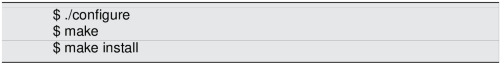
Now, compile the source code as follows:
-
Non MPI users

-
MPI users


This will take a few minutes, depending on your system.
If you got a “Compilation done” message on your terminal, you are ready to run your first example.
3.4 Update OpenPhase
OpenPhase employs standard versioning, although it is continuously under development with frequent updates. We recommend keeping OpenPhase up to date as you use it to develop your application(s); regular upgrades are advised. New and archived versions of the OpenPhase library can be found on our website at https://openphase.rub.de/download.html.
3.5 OpenPhase Application
3.5.1 Structure of an OpenPhase Application
Each application example directory should have at least the following files (Mandatory):
-
ProjectInput.opi
-
Main.cpp
-
Makefile
It may include additional files (Optional):
-
Auxiliary input files (e.g. EBSD, Orientations, Geometry, etc.)
-
Post Processing files (e.g. Gnuplot, python, etc.)
The structure and parameters for the input file, which has been given the name “ProjectInput.opi”, will be discussed in the next section.
3.5.2 Compile Your Application
Compile the application source code as follows:
-
Non MPI users

-
MPI users


If the application is functioning properly, the output won’t indicate errors. Depending on your compiler version, you may get warnings that can usually be disregarded. Be sure to recompile and test your application after making changes to the source code or updating OpenPhase library.
3.5.3 Run Your Application
-
Non MPI users

-
MPI users


This command tells the computer to run the executable program “ApplicationName” on 4 CPUs.
Note: This mpirun command may be useful for novices with simple tasks, but it’s not the way to go when you have a large, lengthy application! Additionally, outcomes can vary from machine to machine. When you request 4 processors, for example,
-
In the best-case scenario, mpirun detects three additional PCs similar to the one you’re using, copies your software to them, and runs it on all four.
-
In a less ideal scenario, your current system has four processors, this memory is shared among them, and your program runs;
-
In the worst-case scenario, there are less than four processors available, therefore one of them will “timeshare” and alternately run two or more of your process.
4 The Input File Structure
OpenPhase is a command-line, non-interactive tool; it anticipates that the simulation input parameters will be provided in the form of an input file. The user must ensure that the input parameters file is placed in the same folder as the simulation example before proceeding. This file is typically referred to as ProjectInput file. The OpenPhase software will read the input file and begin the simulation immediately if the data is correct and sufficient. If this is not the case, then OpenPhase will show an error message and expect the user to correct the input file independently.
4.1 Step by Step Through the ProjectInput File
This section will walk through a default ProjectInput file line by line, explaining exactly what each line does and what it represents.
4.1.1 RunTimeControl
The input file begins with the RunTimeControl module input. This controls the simulation time, the frequency of outputs, and whether the user wants to start a new simulation or restart an existing simulation from a specific time step. Figure 9.1 shows all the parameters related to the RunTimeControl module. The following gives a description of each parameter:

The RunTimeControl section in the ProjectInput file
— SimTtl
The user can specify a title for the simulation.
— nSteps
The number of time steps for the entire simulation. To calculate the actual time, you have to multiply this number by Δt.
— FTime, STime
Sets parameters for the frequency of data output to the disk (FTime) and to the screen (STime).
— LUnits, TUnits, MUnits
All the values are in the SI system of units, which uses the meter, second, and kilogram as base units.
— dt
This is the initial time step (time discretization) Δt. Note that some modules might use an internal time-stepping scheme.
— nOMP
The number of OpenMP threads can be specified if you want to run your simulation in a multithreading mode. The number 1 indicates no active multithreading. Make sure to understand how OpenMP works before running your simulation using multithreading because if you increase it unwisely, it can slow your simulation instead of making it faster.
— Restrt
OpenPhase gives the user the option of either starting a new simulation (No) or restarting from the existing previously saved output (Yes).
— tStart
Suppose you indicate (Yes) in the previous option. In that case, you have to specify the time step from which you want to restart your simulation.
— tRstrt
Set parameter for the frequency of raw-data output to the disk for restarting.
4.1.2 Settings
The Settings input controls the size and numerical resolution of the simulation domain, and the user must specify the grid spacing and the number of grid points along each dimension. The grid spacing is one of the most critical numerical parameters because it defines the resolution of the simulation. In practice, high resolution means more time, so it is usually necessary to find a middle ground between grid resolution and calculation time. Other information linked to the phases is contained inside the Settings parameters, including the thermodynamic phase of each phase field and various additional information about the phases, such as their aggregate state (solid, liquid, or gas) and the chemical components, among other things, as shown in Fig. 9.2.

The Settings section in the ProjectInput file
— Nx, Ny, Nz
The simulation system size in the x, y, and z directions given in grid points.
— dx
Sets the grid spacing Δx. It is important to note that this value is the same for all three spatial dimensions.
— iWidth
The interface width η of the phase field given in grid points.
— Phase
The name of the phase; the running index refers to the thermodynamic phase for a given phase field.
— State
The aggregate state of the phase (solid, liquid, or gas).
— Comp
The chemical component name.
— Nvariants
The number of crystallographic (symmetry/translation/...) variants for a given phase.
4.1.3 BoundaryConditions
The boundary conditions of the simulation domain have to be set individually for every simulations domain side in the ProjectInput file, as shown in Fig. 9.3.

The BoundaryConditions section in the ProjectInput file
— BCN0X, BCNX, BCN0Y, BCNY, BCN0Z, BCNZ
These keywords define the six individual sides of the calculation domain.
In OpenPhase The following boundary conditions are available:
-
Periodic: Periodic boundary conditions.
-
NoFlux: Adiabatic boundary conditions, resulting in zero first-order derivative at the boundary.
-
Free: Boundary conditions resembling a free surface, resulting in a continuous gradient across the boundary.
-
Fixed: Fixed (Dirichlet or Neumann) boundary conditions. The value should be set by the user.
Author information
Authors and Affiliations
Rights and permissions
Open Access This chapter is licensed under the terms of the Creative Commons Attribution 4.0 International License (http://creativecommons.org/licenses/by/4.0/), which permits use, sharing, adaptation, distribution and reproduction in any medium or format, as long as you give appropriate credit to the original author(s) and the source, provide a link to the Creative Commons license and indicate if changes were made.
The images or other third party material in this chapter are included in the chapter's Creative Commons license, unless indicated otherwise in a credit line to the material. If material is not included in the chapter's Creative Commons license and your intended use is not permitted by statutory regulation or exceeds the permitted use, you will need to obtain permission directly from the copyright holder.
Copyright information
© 2023 The Author(s)
About this chapter

Cite this chapter
Steinbach, I., Salama, H. (2023). Tutorial 1: OpenPhase. In: Lectures on Phase Field . Springer, Cham. https://doi.org/10.1007/978-3-031-21171-3_9
Download citation
DOI: https://doi.org/10.1007/978-3-031-21171-3_9
Published:
Publisher Name: Springer, Cham
Print ISBN: 978-3-031-21170-6
Online ISBN: 978-3-031-21171-3
eBook Packages: Chemistry and Materials ScienceChemistry and Material Science (R0)