Tutorial 2: OpenPhase Examples

Abstract

For the purpose of numerically exploring different microstructure evolution processes, the phase-field approach has been developed. Large domains and adequate models that combine many physical fields in statistically relevant volume elements are needed to describe these complicated processes accurately. In order to facilitate such development for multi-physics simulations, OpenPhase was developed for application in material science and engineering. This chapter presents two examples simulated using the OpenPhase software, grain growth and dendritic solidification. The corresponding input files for OpenPhase are listed and explained. Also, some hints for postprocessing are given.

1 Normal Grain Growth

Grain growth is a microstructure-evolution phenomenon that occurs in polycrystalline materials after solidification. In this process, some grains are growing at the cost of the shrinkage of other grains or crystallites of a specific orientation. Consequently, the average grain size increases, and the number of grains in the material decreases.

Grain growth is curvature-driven grain-boundary motion between different crystallites with different orientations. The energy of these grain boundaries adds excess free energy to the system. Therefore, the reduction of the grain-boundary energy is the driving force for the movement of the grain boundaries, and the system evolves towards minimizing the total free energy.

As a result, the material’s microstructure proceeds to reduce the total interface area. The kinetics of grain boundaries influence the interfacial migration; the energy and mobility of these boundaries control how the grain structure evolves.

1.1 Simulation Example

The OpenPhase distribution comes with the NormalGG example, which demonstrates the simulation of grain growth. The driving force is curvature, which is the only contribution to the microstructure evolution. Other contributions, such as temperature and concentration, can easily be coupled.

The example shows normal grain growth with isotropic interface energy and mobility, and the user can modify the example to account for the anisotropy of both contributions.

The microstructure is generated using Voronoi tessellation. The initial number of grains can be changed directly by the user in the example file. The ProjectInput.opi file contains all the input parameters related to the simulation, and the user can modify it for different applications. In this simulation, random crystallographic orientations are assigned to all grains. Periodic boundary conditions are introduced in all directions. The other simulation parameters are listed in Table 10.1.

Table 10.1 Simulation parameters

The reader can find the source code of this example in the OpenPhase distribution in the examples folder. The source code is also included in this chapter (Listing 2). Warning: the code presented here is only for illustration and is subject to changes in the future. The reader is therefore referred to the OpenPhase website for the actual documentation.

1.1.1 Step by Step Through the Source Code

Lines 1–23: :

Importing different classes from the OpenPhase library that are used in the simulation of this example.

Lines 26–28: :

This function sets the initial microstructure as shown in Fig. 10.1b. In this illustrative example, 200 grains have been initialized with the same thermodynamic phase but different phase-field indices based on the Voronoi tessellation technique implemented in the Initializations class. The grains have a random crystallographic orientation, indicated by the RGB colors in Fig. 10.1a.

Fig. 10.1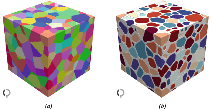

Initial microstructure, displayed in different modes: (a) RGB colors; (b) as phase-field index, where the diffuse interface region is displayed in light grey

Line 32: :

This function sets the interface properties: mobility and energy. In this example, isotropic interface energy and mobility have been used, as shown in Fig. 10.2. However, the user can use different anisotropy model forces for the interface energy and mobility in the ProjectInput file.

Fig. 10.2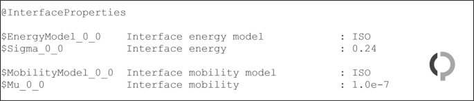

The InterfaceProperties module in the ProjectInput file

Line 33: :

This function calculates the interface-curvature-related driving force. It includes the multi-junction energy as indicated in Eq. (6.1).

Line 34: :

This function limits the phase-field increments for all present phase-field pairs so that the actual phase-field values are within their natural limits of 0 and 1.

Line 35: :

This function merges the increments into the phase fields. It finalizes the phase-field calculations by setting the boundary conditions, calculating the derivatives, setting the flags that mark interfaces, collecting the volume for each phase field, and calculating the thermodynamic phase fractions.

Line 39: :

This function writes an output file in VTK format, which contains the information of the phase field (such as the interfaces, the junctions, and the phase fractions of the different phases). III ParaView can be used to visualize the VTK files, and the output results can be seen in Fig. 10.3.

Fig. 10.3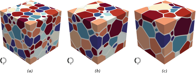

Evolution of the microstructure at different times t (in time steps). (a) t = 500. (b) t = 1500. (c) t = 3000

Lines 41–47: :

This code block prints different simulation information on the screen.

Listing 1 Source code for the NormalGG example in OpenPhase

1.1.2 Results

Figure 10.3 shows the microstructural evolution for the given parameters, in which the grain boundaries appear as grey regions separating individual grains.

2 Dendritic Solidification

Phase-field simulation can be used to model the solidification of metallic alloys. Interface velocities are well represented by a Gibbs–Thomson relation. This is known as the Stefan problem when linked to heat and solute redistribution at the interface and long-range transport in bulk phases. Interfacial energy anisotropy is weak and can be considered a perturbation of a spherical Wulff shape. Even though the solid and liquid have different densities, no significant stresses are developed at the interface during growth. In comparison to solute diffusion in the melt, heat conduction in both phases is almost the same, and solute diffusion in the solid can be ignored [1]. In general, the evolution of the dendrite interface area is characterized by a rapid increase during the growth of side branches, and this is followed by a decrease due to capillarity and coalescence of adjacent structures.

2.1 Simulation Example

The OpenPhase distribution provides the SolidificationFeC example, which is a simulation of dendritic solidification.¹ The code presented here is written considering a 2D case. However, it can be modified to account for the 3D case. In this example, two different simulations have been considered: 2D equiaxed dendritic solidification for a single grain and for multiple grains with different orientations growing from the melt.

The reader can find the source code for this example in the OpenPhase distribution in the examples folder. The source code is also included in the chapter (Listing 2). Warning: the code presented here is only for illustration and is subject to changes in the future. Therefore, the reader is referred to the OpenPhase website for the actual documentation.

Listing 2 Source code for the SolidificationFeC example in OpenPhase

2.1.1 Step by Step Through the Source Code

1: Equiaxed Dendritic Solidification for a Single Grain

Lines 1–30: :

Importing different classes from the OpenPhase library that are used in the simulation of this example.

Lines 32–35: :

These functions set the initial microstructure as illustrated in Fig. 10.4a. There is a matrix with a single phase representing the liquid, which has a phase index equal to 0, and we plant a grain nucleus in the middle of our simulation domain, which represents the solid phase and has a phase index equal to 1.

Fig. 10.4

Equiaxed dendritic solidification in 2D. (a) t = 0.05 s. (b) t = 0.25 s. (c) t = 0.75 s. (d) t = 1.5 s

Lines 37–38: :

These functions set the initial composition, and the temperature and diffusion coefficients for the system. They take their inputs from the ProjectInput file.

Line 44: :

This function sets the interface properties: mobility and energy. In this example, anisotropic driving forces for the interface energy and mobility have been set in the ProjectInput file.

Line 45: :

This function calculates concentration-dependent mobility.

Line 46: :

This function calculates the interface-curvature-related driving force. It includes the triple-junction energy as indicated in Eq. (6.1).

Line 47: :

This function calculates the driving force for each point.

Line 48: :

This function averages the driving forces across the interface.

Line 50: :

This function calculates a time-independent phase-field increment by converting the local driving forces. An additional noise term can be applied, as can a stability mechanism to strengthen the numerical phase-field profile.

Line 51: :

This function limits phase-field increments for all present phase-field pairs so that the actual phase-field values are within their natural limits of 0 and 1.

Line 52: :

This function calculates the change of total concentrations in one time step taking into account cross terms.

Line 53: :

This function sets the temperature according to the cooling rate; it applies equal temperature increments to all points.

Line 54: :

This function merges the increments into the phase fields. It finalizes the phase-field calculations by setting the boundary conditions, calculating the derivatives, setting the flags that mark interfaces, collecting the volume of each phase field, and calculating the thermodynamic phase fractions.

Lines 57–65: :

This code block writes different output files in VTK format, which contains the information of the phase field (such as the interfaces, the junctions, and the phase fractions of the different phases), composition, temperature, and interface properties. III ParaView can be used to visualize the VTK files.

Lines 66–74: :

This code block prints different simulation information on the screen.

2: Equiaxed Dendritic Solidification for Multiple Grains with Different Orientations

For this case, the code stays the same as discussed above with a little modification to the initialization part, in which line 34 can be replaced by the following line:

This function plants random nucleation sites in the simulation domain with different orientations. The number of particles can be chosen by replacing NoOfParticles with an integer number.

2.1.2 Results

Figures 10.4 and 10.5 show that side branches emerge as the dendritic tips extend into the undercooled melt, resulting in a complicated solid–liquid interface morphology. Once you reach a certain distance behind the dendritic tip, a slower evolution begins to take place, which occurs at or around the point of phase equilibrium. Capillarity and delayed solidification play a significant role in determining the interface dynamics at this stage.

Fig. 10.5

Equiaxed dendritic solidification of multiple grains with different orientations. (a) t = 0.05 s. (b) t = 0.25 s. (c) t = 0.75 s. (d) t = 1.5 s