Random Variables and Stochastic Processes

Abstract

Randomness enters into communications problems through the classes of sources, such as speech, images, and music, that we wish to send from one location to another, as well as through the types of distortions, such as additive noise, phase jitter, and fading, that are inserted by real channels. Randomness is the essence of communications; it is that which makes communications both difficult and interesting. Everyone has an intuitive idea as to what "randomness" means, and in this chapter we develop different ways to characterize random phenomena that will allow us to account for randomness in both sources and channels in our communication system analyses and designs.

Appendices

Summary

In this chapter we have briefly surveyed the topics of probability, random variables, and stochastic processes. This material is the absolute minimum knowledge required of these fields to continue our study of communication systems.

Problems

• 4.1 A binary data source S produces 0’s and l’s independently with probabilities P(0) = 0.2 and P(1) = 0.8. These binary data are then transmitted over a noisy channel that reproduces a 0 at the output for a 0 in with probability 0.9, that is, P$\left( {0|0} \right)$ = 0.9. The channel erroneously produces a 0 at its output for a 1 in with probability 0.2, that is, P$\left( {0|1} \right)$= 0.2.

  • (a) Find $P\left( {1|0} \right)$ and $P\left( {1|1} \right)$.

  • (b) Find the probability of a 0 being produced at the channel output.

  • (c) Repeat part (b) for a 1.

  • (d) If a 1 is produced at the channel output, what is the probability that a 0 was sent?

• 4.2 Rework Example 4.2.1 if $P\left( {\xi_{1} } \right) = 0.1$, $P\left( {\xi_{2} } \right) = 0.3$, $P\left( {\xi_{3} } \right) = 0.5$, and $P\left( {\xi_{4} } \right) = 0.1.$

• 4.3 For Example 4.2.1, define the random variables $X\left( {\xi_{1} } \right) = 0,X\left( {\xi_{2} } \right) = 1,X\left( {\xi_{3} } \right) = 2,$ and $X\left( {\xi_{4} } \right) = 3$. Find and sketch the cumulative distribution function and the probability density function for this random variable.

• 4.4 Suppose that for Example 4.2.1, we are only interested in the number of telephones in use at any time. Hence we are led to define the random variable $X\left( {\xi_{1} } \right) = 0,X\left( {\xi_{2} } \right) = 1,X\left( {\xi_{3} } \right) = 1,$ and $X\left( {\xi_{4} } \right) = 2$. Write and sketch the cumulative distribution function and the probability density function for this random variable.

• 4.5 We consider the random experiment of observing whether three telephones in an office are busy or not busy. The outcomes of this random experiment are thus:

  $\xi_{1}$ = no telephones are busy.

  $\xi_{2}$ = only telephone 1 is busy.

  $\xi_{3}$ = only telephone 2 is busy.

  $\xi_{4}$ = only telephone 3 is busy.

  $\xi_{5}$ = telephones 1 and 2 are busy but 3 is not busy.

  $\xi_{6}$ = telephones 1 and 3 are busy but 2 is not busy.

  $\xi_{7}$ = telephones 2 and 3 are busy but 1 is not busy.

  $\xi_{8}$ = all three telephones are busy.

  The probabilities of these outcomes are given to be $P\left( {\zeta_{1} } \right) = 0.3,P\left( {\zeta_{2} } \right) = P\left( {\zeta_{3} } \right) = P\left( {\zeta_{4} } \right) = 0.1,P\left( {\zeta_{5} } \right) = P\left( {\zeta_{6} } \right) = P\left( {\zeta_{7} } \right) = 0.02$ and $P\left( {\zeta_{8} } \right) = 0.34$.

  • (a) What is the probability of the event that one or more telephones are busy?

  • (b) What is the probability that telephone 3 is in use?

  • (c) Consider the event that telephone 3 is busy and the event that only telephones 1 and 2 are busy. Are these two events statistically independent?

• 4.6 Suppose that for the random experiment in Problem 4.5, we are only interested in the number of telephones in use at any time. Define an appropriate random variable, find its cumulative distribution function and probability density function, and sketch both functions.

• 4.7 Given the distribution function of the discrete random variable Z,

  $$ F_{Z} (z) = \left\{ {\begin{array}{*{20}l} {0,} \hfill & {z < 0} \hfill \\ {\frac{1}{4},} \hfill & {0 \le z < 2} \hfill \\ {\frac{3}{8},} \hfill & {2 \le z < 3} \hfill \\ {\frac{1}{2},} \hfill & {3 \le z < 5} \hfill \\ {\frac{7}{8},} \hfill & {5 \le z < 8} \hfill \\ {1,} \hfill & {z \ge 8.} \hfill \\ \end{array} } \right. $$

  • (a) Sketch F_Z(z).

  • (b) Write an expression for F_Z(z).

  • (c) Write an expression for and sketch the pdf of Z.

  • (d) Find P[Z < 2], P[Z $\leq$ 2], and P[2 < Z $\leq$ 8].

• 4.8 The cumulative distribution function of a continuous random variable Y is sketched in Fig. PA.8.

  • (a) Write an expression for F_Y(y).

  • (b) Find an expression for and sketch the pdf of Y.

  • (c) Find P[Y ≤ 1], P[Y ≤ 3], and P[2 < Y ≤ 5].

  

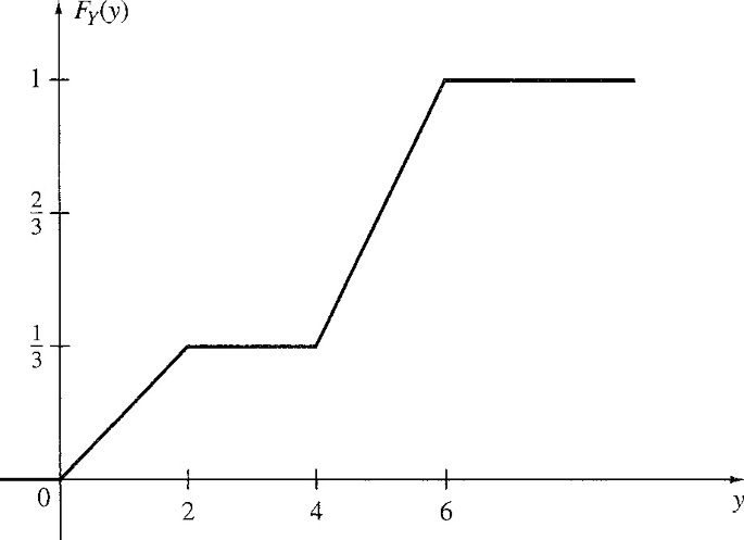
  Fig. PA.8 Cumulative distribution function

• 4.9 Given the joint probability density function

  $$ f_{XY} \left( {x,y} \right) = \left\{ {\begin{array}{*{20}l} {Ke^{{ - {{\left( {3x + 2y} \right)} \mathord{\left/ {\vphantom {{\left( {3x + 2y} \right)} 6}} \right. \kern-0pt} 6}}} ,} \hfill & {x \ge 0,} \hfill & {y \ge 0} \hfill \\ {0,} \hfill & {x < 0,} \hfill & {y < 0.} \hfill \\ \end{array} } \right. $$

  • (a) Find K such that f_XY(x, y) is a valid pdf.

  • (b) Find an expression for F_XY(x, y).

  • (c) Find the marginal distribution and density functions of X.

  • (d) Calculate P[X ≤ 1, Y ≤ 1].

  • (e) Calculate P[X ≤ 2, Y > 1].

• 4.10 Are the random variables X and Y in Problem 4.9 statistically independent? Use both distribution and density functions to substantiate your answer.

• 4.11 Given the joint pdf of Y and Z.

  $$ f_{YZ} \left( {y,z} \right) = \left\{ {\begin{array}{*{20}l} {\frac{3y}{2} + \frac{z}{2},} \hfill & {0 \le y \le 1,\quad 0 \le z \le 1} \hfill \\ {0,} \hfill & {{\text{otherwise}}.} \hfill \\ \end{array} } \right. $$

  • (a) Find the marginal densities of Y and Z.

  • (b) Find $f_{{Y|Z}} \left( {y|Z} \right)$.

  • (c) Calculate $F_{{Y|Z}} \left( {y|Z = z} \right)$.

  • (d) Calculate $F_{Y|Z} \left( {y|z} \right)$.

  • (e) Compare the results of parts (c) and (d).

• 4.12 Given the random variable X with pdf (α a Constant)

  $$ f_{X} \left( x \right) = Ke^{ - \alpha x} u\left( x \right). $$

• (a) Find K in terms of α.

• (b) Calculate E[X], E[X²], and var(X).

• (c) What is $E\left\{ {2X^{2} + 3X + 1} \right\}$?

• 4.13 Compute the characteristic function of the pdf in Problem 4.12 and calculate the moments using Eq. (4.8).

• 4.14 Given the joint pdf

  $$ f_{XY} \left( {x,y} \right) = \left\{ {\begin{array}{*{20}l} {\frac{1}{12}\left( {2 + xy} \right),} \hfill & {0 \le x \le 2,\quad 0 \le y \le 2} \hfill \\ {0,} \hfill & {{\text{otherwise}}.} \hfill \\ \end{array} } \right. $$

• (a) Calculate E{XY}.

• (b) Find cov(X, Y) and p_XY.

• (c) Are X and Y uncorrelated? Orthogonal?

• 4.15 For the joint pdf in Problem 4.11:

• (a) Find E[YZ],

• (b) Find cov(Y, Z) and ${\rho_{XY}}$.

• (c) Are Y and Z uncorrelated? Orthogonal?

• 4.16 Given the discrete random variable Z in Problem 4.7, find the cumulative distribution function and the probability density function of the random variable Y = Z + 2.

• 4.17 The continuous random variable Y has the pdf

  $$ f_{Y} \left( y \right) = \frac{1}{2\sqrt e }e^{{ - {{\left( {y - 1} \right)} \mathord{\left/ {\vphantom {{\left( {y - 1} \right)} 2}} \right. \kern-0pt} 2}}} u\left( y \right). $$

  Find the pdf of the random variable Z = 2Y + 2.

• 4.18 Given the joint pdf of X and Y,

  $$ f_{XY} \left( {x,y} \right) = \left\{ {\begin{array}{*{20}l} {1,} \hfill & {0 < x < 1,\quad 0 < y < 1} \hfill \\ {0,} \hfill & {{\text{otherwise}},} \hfill \\ \end{array} } \right. $$

  Find the joint pdf of the random variables W = X + Y and Z = X − 7.

• 4.19 Two random variables X and Y have the joint pdf

  $$ f_{XY} \left( {x,y} \right) = \left\{ {\begin{array}{*{20}l} {\frac{1}{4}e^{{ - {{\left( {x + y} \right)} \mathord{\left/ {\vphantom {{\left( {x + y} \right)} 2}} \right. \kern-0pt} 2}}} ,} \hfill & {0 \le x < \infty ,\quad 0 \le y < \infty } \hfill \\ {0,} \hfill & {{\text{otherwise}}.} \hfill \\ \end{array} } \right. $$

  We wish to find the pdf of W = X + Y.

  Hint: Use an auxiliary variable.

• 4.20 A double-sided exponential or Laplacian random variable has the pdf

  $$ f_{X} \left( x \right) = K_{1} e^{{ - K_{2} \left| x \right|}} ,\quad \quad - \infty < x < \infty . $$

• (a) For this to be a pdf, how are K₁ and K₂ related? Let K₂ = 1 and find K₁.

• (b) Is X zero mean?

• (c) Compute the variance of X.

• 4.21 Find the characteristic function of the Laplacian random variable

  $$ f_{Y} \left( y \right) = \frac{1}{2\sigma }e^{{ - {{\left| {y - \mu } \right|} \mathord{\left/ {\vphantom {{\left| {y - \mu } \right|} \sigma }} \right. \kern-0pt} \sigma }}} ,\quad \quad - \infty < y < \infty , $$

  where σ > 0. Calculate the mean and variance.

• 4.22 A Gaussian random variable X has the pdf

  $$ f_{X} (x) = \frac{1}{{\sqrt {2\pi } \sigma }}e^{{ - (x - \mu )^{2} /2\sigma^{2} }} ,\quad \quad - \infty < x < \infty . $$

  Find the pdf of the random variable Y = aX + b.

• 4.23 A random variable X has the uniform pdf given by

  $$ f_{X} \left( x \right) = \left\{ {\begin{array}{*{20}l} {\frac{1}{b - a},} \hfill & {a \le x \le b} \hfill \\ {0,} \hfill & {{\text{otherwise}}.} \hfill \\ \end{array} } \right. $$

  • (a) Find the pdf of X₁ + X₂ if X₁ and X₂ are independent and have the same pdf as X.

  • (b) Find the pdf of X₁ + X₂ + X₃ if the X_i, i = 1, 2, 3 are independent and have the same pdf as X.

  • (c) Plot the resulting pdfs from parts (a) and (b). Are they uniform?

• 4.24 Let $Y = \sum\nolimits_{i = 1}^{P} {X_{i} } ,$ where the X_i are independent, identically distributed Gaussian random variables with mean 1 and variance 2. Write the pdf of Y.

• 4.25 Derive the mean and variance of the Rayleigh distribution in Eqs. (4.6.17) and (4.6.18).

• 4.26 Find the mean and variance of the binomial distribution using the characteristic function in Eq. (4.6.24).

• 4.27 For a binomial distribution with n = 10 and p = 0.2, calculate, for the binomial random variable X, P[X ≤ 5] and P[X < 5]. Compare the results.

• 4.28 Use the characteristic function of a Poisson random variable in Eq. (4.6.31) to derive its mean and variance.

• 4.29 A random process is given by X(t) = A_c cos[ω_ct + $\Theta$], where A_c and ω_c are known constants and $\Theta$ is a random variable that is uniformly distributed over [0, 2π].

  • (a) Calculate E[X(t)] and R_X(t₁, t₂).

  • (b) Is X(t) WSS?

• 4.30 For the random process $Y\left( t \right) = Ae^{ - t} {\text{u}}\left( t \right){,}$ where A is a Gaussian random variable with mean 2 and variance 2,

  • (a) Calculate E[Y(t)], R_Y(t₁, t₂), and var[Y(t)].

  • (b) Is Y(t) stationary? Is Y(t) Gaussian?

• 4.31 Let X and Y be independent, Gaussian random variables with means μ_x and μ_y and variances $\sigma_{x}^{2} \;{\text{and}}\;\sigma_{y}^{2} ,$ respectively. Define the random process $Z\left( t \right) = X\cos \omega_{c} t + Y\sin \omega_{c} t,$ where ω_c is a constant.

  • (a) Under what conditions is Z(t) WSS?

  • (b) Find f_z(z; t)

  • (c) Is the Gaussian assumption required for part (a)?

• 4.32 A weighted difference process is defined as Y(t) = X(t) − αX(t − ∆), where α and ∆ are known constants and X(t) is a WSS process. Find R_Y(τ) in terms of R_X(τ).

• 4.33 Use the properties stated in Sect. 4.7 to determine which of the following are possible autocorrelation functions for a WSS process (A > 0).

  • (a) $R_{X} \left( \tau \right) = Ae^{ - \tau } u\left( \tau \right)$

  • (b) $R_{X} \left( \tau \right) = \left\{ {\begin{array}{*{20}l} {A\left[ {{{1 - \left| \tau \right|} \mathord{\left/ {\vphantom {{1 - \left| \tau \right|} T}} \right. \kern-0pt} T}} \right],} \hfill & {\left| \tau \right| \le T} \hfill \\ {0,} \hfill & {{\text{otherwise}}} \hfill \\ \end{array} } \right.$

  • (c) $R_{X} \left( \tau \right) = Ae^{ - \left| \tau \right|} ,\quad - \infty < \tau < \infty$

  • (d) $R_{X} \left( \tau \right) = Ae^{ - \left| \tau \right|} \cos \;\omega_{c} \tau ,\quad - \infty < \tau < \infty$

• 4.34 It is often stated as a property of a WSS, nonperiodic process X(t) that

  $$ \mathop {\lim }\limits_{\tau \to \infty } R_{X} \left( \tau \right) = \left( {E\left[ {X(t)} \right]} \right)^{2} . $$

  This follows, since as τ gets large, X(t), X(t + τ) become uncorrelated. Use this property and property 1 in Sect. 4.7 to find the mean and variance of those processes corresponding to valid autocorrelations in Problem 4.33.

• 4.35 Calculate the power spectral densities for the admissible autocorrelation functions in Problem 4.33.

• 4.36 Calculate the power spectral density for Problem 4.31(a).

• 4.37 If ${\mathcal{F}}\left\{ {R_{X} \left( \tau \right)} \right\} = S_{X} \left( \omega \right),$ calculate the power spectral density of Y(t) in Problem 4.32 in terms of S_X(ω).

• 4.38 A WSS process X(t) with R_x(τ) = V$\delta(\tau)$ is applied to the input of a 100% roll-off raised cosine filter with cutoff frequency ω_co. Find the power spectral density and autocorrelation function of the output process Y(t).

• 4.39 A WSS signal S(t) is contaminated by an additive, zero-mean, independent random process N(t). It is desired to pass this noisy process S(t) + N(t) through a filter with transfer function H(ω) to obtain S(t) at the output. Find an expression for H(ω) in terms of the spectral densities involving the input and output processes.

References

Gray, R. M., and L. D. Davisson. 1986. Random Processes: A Mathematical Approach for Engineers. Englewood Cliffs, N.J.: Prentice Hall.
Franks, L. E. 1969. Signal Theory. Englewood Cliffs, N. J.: Prentice Hall.
Author information
Authors and Affiliations
Corresponding author