Orthogonal Functions and Fourier Series

Abstract

Fundamental to the practice of electrical engineering and the study of communication systems is the ability to represent symbolically the signals and waveforms that we work with daily. The representation of these signals and waveforms in the time domain is the subject of this chapter. On first thought, writing an expression for some time function seems trivial; that is, everyone can write equations for straight lines, parabolas, sinusoids, and exponentials. Indeed, this knowledge is important, and it is precisely this ability to write expressions for and to manipulate familiar functions that we will draw on heavily in the sequel. Here, however, we are interested in the extension of this ability to include more complex, real-world waveforms, such as those that might be observed using an oscilloscope at the input or output of a circuit or system.

Appendices

Summary

In this chapter we have expended substantial time and effort in motivating, defining, and developing the idea of a Fourier series representation of a signal or waveform. In Sect. 1.2 we provided the initial motivation and introduced sets of functions that possess the property of orthogonality. The two most important forms of Fourier series for our purposes, the trigonometric and the complex exponential forms, were presented in Sects. 1.3 and 1.4, respectively, and their use illustrated. In Sects. 1.5 and 1.6 we concentrated on simplifying the Fourier series calculations and supplying some previously ignored mathematical details. The important concept of a spectrum of a periodic signal was introduced in Sect. 1.7 and examples were given to clarify calculations. As we shall see, Sect. 1.7 serves as a critical stepping-stone to the definition of the Fourier transform in Chap. 2.

Problems

• 1.1 For the two vectors ${\mathbf{B}}_{0} = 3{\hat{\mathbf{a}}}_{x} + 4{\hat{\mathbf{a}}}_{y}$ and ${\mathbf{B}}_{1} = - {\hat{\mathbf{a}}}_{x} + 2{\hat{\mathbf{a}}}_{y}$, determine the component of B₀ in the ${\mathbf{B}}_{1}$ direction and the component of ${\mathbf{B}}_{1}$ in the B₀ direction.

• 1.2 Determine whether each of the following sets of vectors is orthogonal. Are they orthonormal?

  • (a) ${\mathbf{B}}_{0} = - {\hat{\mathbf{a}}}_{x} + {\hat{\mathbf{a}}}_{y}$ and ${\mathbf{B}}_{1} = {\hat{\mathbf{a}}}_{x} - {\hat{\mathbf{a}}}_{y} .$

  • (b) ${\mathbf{B}}_{0} = - {\hat{\mathbf{a}}}_{x} + {\hat{\mathbf{a}}}_{y}$ and ${\mathbf{B}}_{1} = - {\hat{\mathbf{a}}}_{x} - {\hat{\mathbf{a}}}_{y} .$

  • (c) ${\mathbf{B}}_{0} = {{\left( {{\hat{\mathbf{a}}}_{x} + {\hat{\mathbf{a}}}_{y} } \right)} \mathord{\left/ {\vphantom {{\left( {{\hat{\mathbf{a}}}_{x} + {\hat{\mathbf{a}}}_{y} } \right)} {\sqrt 2 }}} \right. \kern-\nulldelimiterspace} {\sqrt 2 }}$ and ${\mathbf{B}}_{1} = {{\left( {{\hat{\mathbf{a}}}_{x} - {\hat{\mathbf{a}}}_{y} } \right)} \mathord{\left/ {\vphantom {{\left( {{\hat{\mathbf{a}}}_{x} - {\hat{\mathbf{a}}}_{y} } \right)} {\sqrt 2 }}} \right. \kern-\nulldelimiterspace} {\sqrt 2 }}$.

• 1.3 We desire to approximate the vector

  $${\mathbf{A}}_{1} = 4{\hat{\mathbf{a}}}_{x} + {\hat{\mathbf{a}}}_{y} + 2{\hat{\mathbf{a}}}_{z}$$

  by a linear combination of the vectors y₁ and y₂,

  $${\mathbf{A}}_{1}^{\prime } = d_{1} {\mathbf{y}}_{1} + d_{2} {\mathbf{y}}_{2} ,$$

  where ${\mathbf{y}}_{1} = - {\hat{\mathbf{a}}}_{x} + {\hat{\mathbf{a}}}_{y}$ and ${\mathbf{y}}_{2} = - {\hat{\mathbf{a}}}_{x} - {\hat{\mathbf{a}}}_{y}$. Find the coefficients d₁ and d₂ such that the approximation minimizes the least squares loss function given by $\varepsilon^{2} = \left| {{\mathbf{A}}_{1} - {\mathbf{A}}_{1}^{\prime } } \right|^{2}$.

• 1.4 Complete Example 1.2.1 by considering cases (2) and (3).

• 1.5 A set of functions $\left\{ {f_{n} \left( x \right)} \right\}$ is said to be orthogonal over the interval (a, b) with respect to the weighting function $\rho \left( x \right)$ if the functions $\rho^{{{1 \mathord{\left/ {\vphantom {1 2}} \right. \kern-\nulldelimiterspace} 2}}} \left( x \right)f_{n} \left( x \right)$ and $\rho^{{{1 \mathord{\left/ {\vphantom {1 2}} \right. \kern-\nulldelimiterspace} 2}}} f_{m} \left( x \right),m \ne n$, are orthogonal, and thus

  $$\int_{a}^{b} \rho \left( x \right)f_{n} \left( x \right)f_{m} \left( x \right)dx = 0.$$

  The set of polynomials $\left\{ {H_{n} \left( x \right)} \right\}$ defined by the equations

  $$H_{n} \left( x \right) = \left( { - 1} \right)^{n} e^{{{{x^{2} } \mathord{\left/ {\vphantom {{x^{2} } 2}} \right. \kern-\nulldelimiterspace} 2}}} \frac{{d^{n} }}{{dx^{n} }}e^{{ - {{x^{2} } \mathord{\left/ {\vphantom {{x^{2} } 2}} \right. \kern-\nulldelimiterspace} 2}}} ,\;\;\;{\kern 1pt} {\text{ for }}n = 0,1,2, \ldots$$

  are called Hermite polynomials and they are orthogonal over the interval $- \infty < x < \infty$ with respect to the weighting function $e^{{ - {{x^{2} } \mathord{\left/ {\vphantom {{x^{2} } 2}} \right. \kern-\nulldelimiterspace} 2}}}$. Specifically, this says that the two functions $e^{{ - {{x^{2} } \mathord{\left/ {\vphantom {{x^{2} } 4}} \right. \kern-\nulldelimiterspace} 4}}} H_{m} \left( x \right)$ and $e^{{ - {{x^{2} } \mathord{\left/ {\vphantom {{x^{2} } 4}} \right. \kern-\nulldelimiterspace} 4}}} H_{n} \left( x \right),n \ne m$, are orthogonal, so that

  $$\int_{ - \infty }^{\infty } {e^{{ - {{x^{2} } \mathord{\left/ {\vphantom {{x^{2} } 2}} \right. \kern-\nulldelimiterspace} 2}}} } H_{m} \left( x \right)H_{n} \left( x \right)dx = 0.$$

  Show that $H_{0} \left( x \right)$ and $H_{1} \left( x \right)$ satisfy the relation above.

• 1.6 A set of polynomials that are orthogonal over the interval $- 1 \le t \le 1$ without the use of a weighting function, called Legendre polynomials, is defined by the relations

  $$P_{n} \left( t \right) = \frac{1}{{2^{n} n!}}\frac{{d^{n} }}{{dt^{n} }}\left( {t^{2} - 1} \right)^{n} ,\;\;\;{\kern 1pt} {\text{ for }}n = 0,1,2, \ldots$$

  and thus

  $$P_{0} \left( t \right) = 1,\;\;\;{\kern 1pt} P_{1} \left( t \right) = t,\;\;\;{\kern 1pt} P_{2} \left( t \right) = \left( \frac{1}{2} \right)\left( {3t^{2} - 1} \right),$$

  and so on. Legendre polynomials are very closely related to the set of polynomials $\left\{ {1,t,t^{2} , \ldots ,t^{n} , \ldots } \right\}$ that we found to be nonorthogonal in Sect. 1.2. In fact, by using a technique called the Gram-Schmidt orthogonalization process [Jackson, 1941; Kaplan, 1959], the normalized Legendre polynomials, which are thus orthonormal, can be generated.

  Calculate for the Legendre polynomials with $n = 0,1,2$, and so on, as necessary the value of

  $$\int_{ - 1}^{1} {P_{n}^{2} } \left( t \right)dt$$

  and hence use induction to prove that

  $$\int_{ - 1}^{1} {P_{n}^{2} } \left( t \right)dt = \frac{2}{2n + 1}.$$

  Notice that this shows that the Legendre polynomials are not orthonormal. Based on these results, can you construct a set of polynomials that are orthonormal?

• 1.7 Show that the trigonometric functions in Example 1.2.1 are not orthonormal over ${{t_{0} \le t \le t_{0} + 2\pi } \mathord{\left/ {\vphantom {{t_{0} \le t \le t_{0} + 2\pi } {\omega_{0} }}} \right. \kern-\nulldelimiterspace} {\omega_{0} }}$. From these results deduce a set of orthonormal trigonometric functions. Repeat both of these steps for the exponential functions in Example 1.2.2.

• 1.8 Notice that any polynomial in t can be expressed as a linear combination of Legendre polynomials. This fact follows straightforwardly from their definition in Problem 1.6, since we then have

  $$1 = P_{0} \left( t \right),\;\;\;{\kern 1pt} t = P_{1} \left( t \right),\;\;\;{\kern 1pt} t^{2} = \frac{2}{3}P_{2} \left( t \right) + \frac{1}{3}P_{0} \left( t \right),\;\;\;{\kern 1pt} t^{3} = \frac{2}{5}P_{3} \left( t \right) + \frac{3}{5}P_{1} \left( t \right),$$

  and so on. The reader should verify these statements. Using this result, then, we observe that the Legendre polynomial $P_{n} \left( t \right)$ is orthogonal to any polynomial of degree $n - 1$ or less over $- 1 \le t \le 1.$. That is, for g(t) a polynomial in t of degree $n - 1$ or less,

  $$\int_{ - 1}^{1} {P_{n} } \left( t \right)g\left( t \right)\;dt = 0.$$

  Demonstrate the validity of this claim for $n = 4$ and $g\left( t \right) = 5t^{3} - 3t^{2} + 2t + 7.$

• 1.9 Determine the trigonometric Fourier series expansion for the periodic function shown in Fig. P1.9 by direct calculation.

  Fig. P1.9

  

  Determine the trigonometric Fourier series expansion for the periodic function by direct calculation

• 1.10 Obtain the trigonometric Fourier series representation of the waveform in Fig. P1.10.

  Fig. P1.10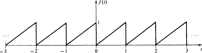

  

  Obtain the trigonometric Fourier series representation of the waveform

• 1.11 Derive the magnitude-angle form of a trigonometric Fourier series given by

  $$f\left( t \right) = a_{0} + \sum\limits_{n = 1}^{\infty } {d_{n} } \cos \left[ {\frac{2\pi nt}{T} + \theta_{n} } \right]$$

  with

  $$d_{n} = 2\left| {c_{n} } \right| = \sqrt {a_{n}^{2} + b_{n}^{2} }$$

  and

  $$\theta_{n} = \tan^{ - 1} \frac{{{\text{Im}} \left\{ {c_{n} } \right\}}}{{{\text{Re}} \left\{ {c_{n} } \right\}}},$$

  where the c_n are the complex Fourier series coefficients and the a_n and b_n are the trigonometric Fourier series coefficients. Start with Eq. (1.4.3) and use the fact that

  $$c_{n} = \left| {c_{n} } \right|e^{{j/\angle c_{n} }} \;\;\;{\kern 1pt} {\text{ when }}n > 0$$

  and

  $$c_{n} = \left| {c_{n} } \right|e^{{ - j/\angle c_{n} }} \;\;\;{\kern 1pt} {\text{ when }}n < 0$$

  for $f\left( t \right)$ real.

• 1.12 The trigonometric Fourier series coefficients for a half-wave rectified version of $f\left( t \right) = \sin t$ are

  $$a_{n} = \left. {\frac{1}{2\pi }\left[ {\frac{{\cos \left( {n - 1} \right)t}}{n - 1} - \frac{{\cos \left( {n + 1} \right)t}}{n + 1}} \right]} \right|_{0}^{\pi }$$

  and

  $$b_{n} = \left. {\frac{1}{2\pi }\left[ {\frac{{\sin \left( {n - 1} \right)t}}{n - 1} - \frac{{\sin \left( {n + 1} \right)t}}{n + 1}} \right]} \right|_{0}^{\pi } .$$

  These expressions are indeterminate when n = 1.

  • (a) Use Eqs. (1.3.3) and (1.3.4) with $n = 1$ to show that $a_{1} = 0$ and $b_{1} = \frac{1}{2}$, respectively.

  • (b) In evaluating indeterminate forms, a set of theorems from calculus called L’Hospital’s rules sometimes proves useful. Briefly, these rules state that if $\mathop {\lim }\limits_{{x \to x_{0} }} {{f\left( x \right)} \mathord{\left/ {\vphantom {{f\left( x \right)} {g\left( x \right)}}} \right. \kern-\nulldelimiterspace} {g\left( x \right)}}$ is indeterminate of the form 0/0 or ${\infty \mathord{\left/ {\vphantom {\infty \infty }} \right. \kern-\nulldelimiterspace} \infty }$ and $f\left( x \right)$ and $g\left( x \right)$ are differentiable in the interval of interest with $g^{\prime } \left( x \right) \ne 0$, then

    $$\mathop {\lim }\limits_{{x \to x_{0} }} \frac{f\left( x \right)}{{g\left( x \right)}} = \mathop {\lim }\limits_{{x \to x_{0} }} \frac{{f^{\prime } \left( x \right)}}{{g^{\prime } \left( x \right)}}.$$

  Use this rule to find a₁ and b₁ respectively. (See an undergraduate calculus book such as Thomas [1968] for more details on L’Hospital’s rules).

• 1.13 Find the complex Fourier series representation of a nonperiodic function identical to f(t) in Fig. 1.3.1 over the interval $- {{\tau /2 \le t \le \tau } \mathord{\left/ {\vphantom {{\tau /2 \le t \le \tau } 2}} \right. \kern-\nulldelimiterspace} 2}$.

• 1.14 Evaluate the complex Fourier series coefficients for the waveform in Fig. P1.9.

• 1.15 Determine the complex Fourier series representation for the waveform in Fig. P1.10.

• 1.16 Calculate the complex Fourier series coefficients for the periodic signal in Fig. P1.16.

  Fig. P1.16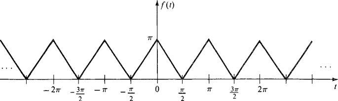

  

  Calculate the complex Fourier series coefficients for the periodic signal

• 1.17 Determine whether each of the waveforms in Fig. P1.17 is even, odd, odd harmonic, or none of these. Substantiate your conclusions.

• 1.18 For the waveforms specified below, determine if any of the symmetry properties discussed in Sect. 1.5 are satisfied. State any conclusions that can be reached concerning the trigonometric and complex Fourier series in each case.

  • (a) Fig. P1.9

  • (b) Fig. P1.10

  • (c) Fig. P1.16

• 1.19 Prove that if $f\left( t \right) = - f\left( {{{t - T} \mathord{\left/ {\vphantom {{t - T} 2}} \right. \kern-\nulldelimiterspace} 2}} \right)$, the complex Fourier series coefficients are zero for $n = 0,2,4, \ldots$

• 1.20 Prove that the integral of an odd function over symmetrical limits is zero; that is, show that if $f\left( t \right) = - f\left( { - t} \right)$, then

  $$\int_{ - a}^{a} f (t)dt = 0.$$

• 1.21 Obtain necessary conditions on the coefficients p₀, p_n, and q_n, n = 1, 2, 3,…, in Eq. (1.6.3) to minimize Eq. (1.6.2). Do these coefficients have any special significance?

  Fig. P1.17

  

  Obtain necessary conditions on the coefficients p₀, p_n, and q_n, n = 1, 2, 3,..., in Eq. (1.6.3) to minimize Eq. (1.6.2). Do these coefficients have any special significance?

• 1.22 Obtain a trigonometric series approximation to $f\left( t \right)$ in Fig. P1.22 such that the total energy remaining in the error is 5% or less of the total energy in $f\left( t \right)$. Do not include any more terms than is necessary.

  Fig. P1.22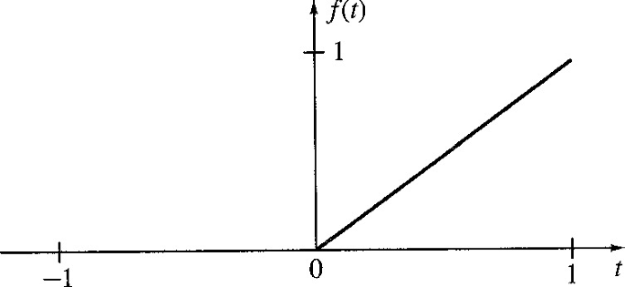

  

  Obtain a trigonometric series approximation to $f\left( t \right)$ in Fig. P1.22 such that the total energy remaining in the error is 5% or less of the total energy in $f\left( t \right)$. Do not include any more terms than is necessary.

• 1.23 Plot the first three partial sums for the Fourier series of Fig. P1.22,

  $$f\left( t \right) = \frac{1}{2} + \sum\limits_{n = 1}^{\infty } {\left( {\frac{ - 1}{{n\pi }}} \right)} \sin 2n\pi t,$$

  on a large sheet of graph paper superimposed on the waveform in Fig. P1.22. What is the value of the integral squared error in this approximation?

• 1.24 What is the trigonometric series approximation to $f(t)$ in Fig. P1.9 such that the energy in the error is 15% or less of the total energy in $f(t)$? Include the fewest terms possible. Plot the resulting approximation over one period and compare to $f(t)$.

• 1.25 Derive Eq. (1.6.11).

• 1.26 Define $r_{N} \left( t \right) = h_{N} \left( t \right) - f_{N} \left( t \right),$, and note that $f\left( t \right) - h_{N} \left( t \right) = f\left( t \right) - f_{N} \left( t \right) - r_{N} \left( t \right)$. Use this last expression in Eq. (1.6.2) to show that f_N(t) is the one out of all possible trigonometric sums of order N that minimizes the ISE.

• 1.27 Derive the expression for the minimum value of the integral squared error in Eq. (1.6.14).

• 1.28 Approximate the waveform in Problem 1.13 by a series of Legendre polynomials of the form $f\left( t \right) = \sum\limits_{n = 0}^{2} {\delta_{n} } P_{n} \left( t \right)$. What percentage of the energy in $f\left( t \right)$ remains in the approximation error if we let $\tau = 1$?

• 1.29 Show that ${\text{Re}} \left\{ {c_{n} } \right\}$ is even and ${\text{Im}} \left\{ {c_{n} } \right\}$ is odd by finding the real and imaginary parts of $c_{n} = \left| {c_{n} } \right|e^{{j/\angle c_{n} }}$ and then using Eqs. (1.7.3) and (1.7.4).

• 1.30 Repeat Problem 1.29 by finding the real and imaginary parts of Eq. (1.4.4).

• 1.31 Find expressions for and sketch the amplitude and phase spectra of $f\left( t \right)$ in Fig. P1.9.

• 1.32 Repeat Problem 1.31 for $f\left( t \right)$ in Fig. P1.10.

• 1.33 Repeat Problem 1.31 for $f\left( t \right)$ in Fig. P1.16.

References

Jackson, D. 1941. Fourier Series and Orthogonal Polynomials. Washington, D.C.: The Mathematical Association of America.
Kaplan, W. 1959. Advanced Calculus. Reading, Mass.: Addison-Wesley.
Author information
Authors and Affiliations
Corresponding author