Dynamical Properties of Weather Regime Transitions

Abstract

Large-scale weather can often be successfully described using a small amount of patterns. A statistical description of reanalysed pressure fields identifies these recurring patterns with clusters in state-space, also called “regimes”. Recently, these weather regimes have been described through instantaneous, local indicators of dimension and persistence, borrowed from dynamical systems theory and extreme value theory. Using similar indicators and going further, we focus here on weather regime transitions. We use 60 years of winter-time sea-level pressure reanalysis data centered on the North-Atlantic ocean and western Europe. These experiments reveal regime-dependent behaviours of dimension and persistence near transitions, although in average one observes an increase of dimension and a decrease of persistence near transitions. The effect of transition on persistence is stronger and lasts longer than on dimension. These findings confirm the relevance of such dynamical indicators for the study of large-scale weather regimes, and reveal their potential to be used for both the understanding and detection of weather regime transitions.

Keywords

1 Introduction

The concept of weather regime was introduced in 1949 by [1]. Broadly speaking, weather regimes are recurring, quasi-stationary states of the atmosphere, which allow to describe most of the subseasonal variability of atmospheric states, the latter being defined through large-scale maps of either mean sea-level pressure or geopotential height. The study of weather regimes has numerous potential applications as a tool to understand subseasonal atmospheric dynamics [2]. The understanding and correct representation of weather regimes is also paramount for adequate climate projections [3].

Vautard [4] defines weather regimes through stationarity and searches for geopotential fields with a quasi-vanishing time-derivative. Others (see e.g. [5]) use cluster analysis (i.e. k-means or Gaussian Mixture Models) to find recurring patterns. To perform such analyses, one usually uses a low-order description of the atmospheric state, through empirical orthogonal functions (EOFs). Some authors simply rely on projection on a low number of EOFs (two in the case of [6]), and on forecaster’s empirical knowledge of the recurrence of regimes defined through positive and negative phases of dominant EOFs.

A natural concern is not only the definition of weather regime, but also the study of their transition [5]. Statistical tools such as random forest can be used to perform such a task [7]. The performance of physics-based weather forecasts can also be assessed through their ability to predict weather regime transitions [6]. Our study of weather regime transition is noticeably motivated by the relevance and difficulty of their forecast.

We aim to focus on the time-evolution of two dynamical indicators (local dimension and persistence) around transitions between winter-time, North-Atlantic weather regimes. These indicators are relevant to the study of Atlantic-European weather regimes, as each weather regime can be associated with specific values of these indicators [8]. From this static study of weather regimes, we carry on with a dynamic study of transitions.

Note, [9] already investigated the temporal behaviour of local dimension and persistence at the mature stage of seven regimes, used to define round-year sub-seasonal variability of weather over the North-Atlantic and western Europe. These mature stages were identified as local minima of the weather regime index defined by [10] as the projection of the instantaneous atmospheric state on the atmospheric state associated with each regime. Hochman et al. [9] showed that the so-defined mature stages of weather regimes coincided with locally low values of the dimension and inverse persistence, and that these mature stages were both preceded and followed by higher relative values of these indicators. The present paper is concerned with weather regime transitions, which are located between weather regime mature stages. We therefore expect to confirm the relatively higher values of dimension and persistence observed by [9] before and after regime mature stages. However, our study could reveal varying behaviours as we focus on transitions from one specific regime to another, while the study of [9] does not specify which regime precedes or follows a given mature stage.

Our analysis also bears similarity with the one of [11], in which the temporal behaviour of local dimension and persistence during Eastern Mediterranean cold spells was examined. The main difference with the present study is the nature of the event of interest: we are interested in transitions between weather regimes, while cold spells could be viewed as a special type of weather regime (a particular case of Cyprus Lows which is the dominant regime responsible for precipitation in the Eastern Mediterranean region).

The next section is the core of our paper and reviews the results of our study, describing salient features of the time-evolution of dimension and persistence around transitions between four winter-time North-Atlantic weather regimes. The following section draws perspectives and proposes potential applications to real-world meteorological issues. Appendix sections provide details to the tools and data used in the present study.

2 European-Atlantic Weather Regime Transitions

An EOF-decomposition is performed (see section “Empirical Orthogonal Functions”) of winter-time, reanalysed sea-level pressure fields described in Appendix 1. A weather-regime analysis follows using a Gaussian Mixture Model with four modes, corresponding to four weather regimes, in a reduced-space spanned by the three first EOFs (see section “Gaussian Mixture Model” for a discussion). The resulting regimes are shown in Fig. 1 in EOF space and there centroids are shown in Fig. 2 as SLP-anomaly maps.

Fig. 1

Weather regimes as cluster distributions from the fit of a Gaussian Mixture Model to winter-time sea-level-pressure anomaly (SLPa) from reanalysis data. The fit is performed in reduced space through projection of SLPa maps on three leading empirical orthogonal functions (EOF). Colored contours show the 0.75σ (thick lines) and 1.25σ (thin lines) ellipses of each distribution around their centroids, with σ denoting standard deviation. Grey contours show the whole GMM distribution through marginal distributions in two-dimenisonal EOF-subspaces. Regime names are assigned from comparison with other scientific studies found in the litterature (see Fig. 2)

Fig. 2

Weather regimes as sea-level-pressure anomalies in (longitude, latitude) coordinates (coastlines are shown), defined by the distributions’ centroids from a Gaussian Mixture Model (see Fig. 1 and section “Gaussian Mixture Model”). Regime names are assigned from comparison with other scientific studies found in the literature

Figure 1 illustrates that the four regimes are mostly defined through EOF1 and EOF2, as the centroids’ EOF3-coordinates are close to zero. Two regimes are associated with positive-negative phases of the first EOF, corresponding to a strong north-south pressure gradient (see Fig. 2), and we label these regimes NAO+  and NAO− to match previous works in the litterature. The two other regimes are associated with a pressure system covering western Europe and extending far-off Europe’s west-coast. The regime corresponding to an anticyclonic situation over western Europe is termed BLO+ , and its opposite phase is termed BLO−, in accordance with previous studies on such regimes. Note that the small contribution of EOF3 to the definition of BLO+  and BLO− induces a slight west-ward shift of the BLO− pressure system compared to the one of BLO+ .

Then, we follow [5] and assign each SLP-anomaly field to a weather regime if it lies inside the 1.25σ ellipses, shown in Fig. 1 (in cases of points belonging to two regimes, we assign the regime with highest probability), otherwise no regime is assigned. Next, for any regimes “A” and “B”, a transition from regime “A” to regime “B” is defined as either the consecutive passing from “A” to “B” or the consecutive passing from “A” to “no regime” and then to “B” (note that this allows transitions from a regime to itself). As we are interested in the behaviour of dynamical indicators around transitions, we discard transitions of the type “A”→“no regime”→“B” if the “no regime” phase exceeds 24 h.

3 Dimensionality Around Transitions

The local dimension of sea-level pressure fields is used as an indicator of the state of the atmosphere. Details on this indicator and how is it computed can be found in section “Local Dimensions”.

In Fig. 3, one observes statistics of dimension-versus-time profiles centered on transitions. The number of transitions on which the statistics were computed is also mentioned, showing preferred transitions in agreement with [5]. Several behaviours can be observed.

Smooth transition :

The transition BLO+  → NAO− shows a smooth transition from the dimension statistics of regime BLO+  to the statistics of regime NAO− over a transition period of ∼1 day, starting after the transition, with no particular behaviour at the transition itself.

Fig. 3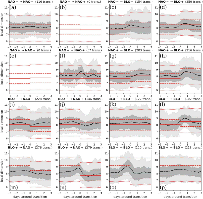

Typical profiles of local dimension versus time, centered at transition point, for each possible transitions. Light (resp. dark) greys fill between the 0.05 and 0.95 (resp. 0.25 and 0.75) quantiles, while the dark lines show the average dimension profile around transition from regime “A” to regime “B”. In red, statistics over each regime (with no restriction to transitions) are shown. Red dotted (resp. dashed) lines show the 0.05 and 0.95 (resp. 0.25 and 0.75) quantiles, while the full red lines show the average dimension of regime “A” and “B”

Dimension overshoot :

Right before, after, or during transitions NAO−→ BLO−, BLO− → BLO+ , BLO+  → BLO−, and BLO+ →NAO+ , the local dimension statistics exceed what is expected from statistics computed over each regime. Transitions BLO− → BLO+  and BLO+  → BLO− show the highest intensity of dimension overshoot (around + 1 in dimension), with the average dimension near transition (black, full) reaching the 0.75 quantile of the regime distributions (dashed, red). For transition BLO− → BLO+ , the overshoot occurs ∼1 day after the transition, while for BLO+ → BLO− it occurs 1 day before. In both cases, transition-statistics (black, grey) are very similar to the BLO− regime-statistics (red), while the overshoot occurs in the BLO+  phase, and is preceded or followed by an undershoot.

Time-symmetry :

From the previous description, it appears that the dimension statistics around transition BLO−→BLO+  are almost symmetric to BLO+ →BLO−: the latter can be recovered from taking the former in reverse-time. Similar types of symmetry can be observed in transitions BLO+ ↔NAO+ , BLO−↔NAO+ , and BLO+ ↔NAO−, although with less confidence.

Time-asymmetry :

On the other hand, the transition NAO−→BLO− shows a slight overshoot of dimension statistics at the transition point while the transition BLO−→NAO− shows an overshoot of dimension statistics away from the transition point (∼2 days before and after).

Auto-transitions are harder to interpret than normal transitions. They correspond to trajectories in phase-space where the system goes from a well-defined regime to a mixed, undefined regime, and then comes back to the initial well-defined regime. It is likely that these auto-transitions actually mix different types of transient behaviours, with different properties. Auto-transition NAO+ →NAO+  seems to show an overshoot of dimension near the transition point, but the number of transitions (57) is small and therefore only low confidence is attributed to these statistics. Other auto-transition statistics are rather smooth and close to the corresponding regime-statistics, which might be due to the fact that auto-transitions mix different types of transient behaviours.

Figure 5b shows dimension statistics for all transitions, excluding auto-transitions. It shows a slight dimension overshoot at the transition point ±1 day. The fact that this overshoot is so small is an indicator of the variety of behaviours near transition, depending on which regimes are involved.

4 Persistence Around Transitions

We now use the inverse persistence θ (also called extremal index) of sea-level pressure fields as an indicator of the state of the atmosphere. Details on this indicator and how is it computed can be found in section “Inverse Persistence θ ”.

In Fig. 4, we show the result of the same procedure followed in the previous section, but replacing the local dimension by the inverse persistence. As these two variables are correlated, the behaviour of inverse persistence resembles the one of dimension around much of the observed transitions. However, the difference between transition-statistics and regime-statistics appear to be more significant for θ than for the dimension, with some special behaviours described below.

Fig. 4

Same as Fig. 3, but for the inverse persistence θ (also called extremal index). High values indicate a rapidly changing dynamical system

Fig. 5

In grey: statistics (0.05, 0.25, 0.75 and 0.95 quantiles, as well as mean) of inverse persistence (a) and local dimension (b) over all transitions, discarding auto-transitions (from regime “A” to “A”). In red: statistics (0.05, 0.25, 0.75 and 0.95 quantiles, as well as mean) over all values from the dataset (winter-time from 1956 to 2015), without restriction to transitions

Transitions to/from BLO+ :

The BLO+  regime-statistics of θ are much higher than the ones of other regimes, with most values concentrated between 0.17 and 0.19, and almost all values above 0.16. We therefore see high variations of θ around transitions from or to BLO+ . However, when one is in the regime BLO+ , either after or before a transition, we do not observe an overshoot as with the dimension. Rather, we see that the transition-statistics match the BLO+  statistics very near the transition point, while they are much lower 2–3 days away from the transition. This means that, in the regime BLO+ , the inverse persistence is much lower either 2–3 days before or 2–3 days after any transition. Also, the values of θ in regimes NAO± and BLO−, up to at least three days around a transition from or to BLO+ , are much higher than expected from intra-regime statistics.

We can interpret these fact using the results of [9] who observed a strong decrease of θ when weather regimes are well-installed. Therefore, what we see in Figs. 3d, h, l, m–p and 4d, h, l, m–p indicates that the systems rapidly exits/enters regime BLO+ , while it needs more time to exit/enter neighbouring regimes when transitioning from or to BLO+ .

BLO–↔  NAO+ :

Although the NAO+  and BLO− intra-regime statistics of θ are significantly different, BLO−↔NAO+  transition-statistics of θ are relatively smooth in time, showing very few variations, and closer to the NAO+  intra-regime statistics. Again, this can be interpreted as a slow transition.

Low-quantiles overshoot :

From Fig. 5, one can see that, while all quantiles of dimension seem to be affected equally around transitions (Fig. 5b), it is mostly the low quantiles of inverse persistence which are affected by transitions (Fig. 5a). That is, values of θ are not expected to be especially large near transitions (compared to average statistics), but small values of θ are expected to be extremely unlikely around transitions.

Already mentioned earlier, we discard transitions “A→B” if the “no regime” phase between regimes “A” and “B” exceeds 24 h. Raising the maximum length of this “no regime” phase allows to find more transitions, and results in a slight smoothing of the profiles of Figs. 3 and 5, but the observed tendencies remain. Reducing the maximum length of the “no regime” phase between regimes “A” and “B” results in slightly sharper, yet noisier profiles (not shown).

5 Conclusion and Perspectives

The analysis of reanalysed sea-level pressure maps covering a large part of the North-Atlantic ocean and western Europe, demonstrates that local dynamical indicators of dimension and persistence display great sensitivity to transitions between weather regimes. In particular, we observe higher values of dimension and lower values of persistence near transitions, which is in agreement both with the early definition of weather regimes (as quasi-stationary, low-order recurring states) and with recent studies of weather regimes through these same two dynamical indicators. The study reveals non-homogeneous behaviour of these indicators near transitions, meaning that different transition show different signatures in terms of time-variation of dimension and persistence. Furthermore, we observe that the fingerprint of transitions is more pronounced for persistence than for dimension, and that it spreads over a larger duration (more than ±3 days for persistence but around ±1.5 day for dimension).

This study, combined with recent studies on weather regimes and dynamical indicators, confirm the relevance of these indicators for the understanding of weather regimes, and even reveal the potential for these indicators to be used in the definition of weather regimes. Present findings also indicate that each transition could be identified through the time-behaviour of dimension and persistence. This has great implications and shall motivate further investigations on how to use these indicators for the purpose of detecting regime transitions. However, for each transition we still observe a great variability of time-profiles of dimension and persistence. This suggests to use a variety of related indicators, and not only these two. Recent studies have used these indicators on separated scales, allowing to explore variations in dimensionality and persistence of small-scale variables [23]. Our current analyses also reveal a signature of large-scale weather regime transitions in the time-variation of small-scale dimension and persistence, however with less intensity than for large-scale dynamical indicators (not shown). We interpret this as a hint that small-scale organization may be necessary to large-scale transitions. Other local indicators also based on analogues such as the ones used by [24] and [25] shall also be considered in an attempt to predict transitions.

Appendices

Appendix 1: Data Description: Twentieth Century Reanalysis

We use data from the 3rd version of the twentieth Century Reanalysis, which combines surface observations of synoptic pressure and NOAA’s Global Forecast System, and prescribes sea surface temperature and sea ice distribution [12].

From this reanalysis we extract the ensemble-mean, sea-Level pressure maps from year 1956 to 2015, at 3h-intervals. We do not use preceding years in order to avoid inconsistency between past, observation-scarce data, and more recent data, better constrained by observations. We could also have selected only data from the satellite era starting in 1979, but this would have diminished the statistical significance of our work.

We focus on a 41×41 grid at 1^∘-resolution covering longitudes 30W≤LON≤10E and latitudes 30N≤LAT≤70N, including western Europe and the eastern part of the North-Atlantic Ocean (see Fig. 2). We use only extended-winter data, from October to March, as is typical in North-Atlantic weather-regime studies (see e.g., [9, 6, 8]).

Appendix 2: Statistical Descriptors

1.1 Empirical Orthogonal Functions

To study winter-time SLP fields, we use the empirical orthogonal function decomposition, also called principal component analysis [13]. It allows to decompose any spatial field (snapshot) of SLP-anomaly (SLPa) onto orthogonal maps (EOFs), ordered by their respective contribution to the total variability in time of SLPa fields. To compute SLPa, we remove a moving seasonal-average using data from ±10 years and ±5 calendar-days, with a Gaussian kernel to give more weight to neighbouring years and calendar days.

In our case, EOFs n^∘1–7 contribute respectively to 41%, 24%, 14%, 5.5%, 4.8%, 2.2% and 1.5% of the total signal variance. No that, for our analyses of weather regimes, we use only EOFs n^∘1–3, which contribute collectively to 79% of the total variance.

1.2 Gaussian Mixture Model

A Gaussian Mixture Model (GMM) assumes that the random variable it describes is the result of pooling from a finite number of sub-populations (in our case, regimes) whose distributions are Gaussian [14]. Expectation-maximization (EM) allows to find optimal parameters (averages and covariances) of the Gaussian distributions, once the number of regimes has been fixed.

We follow [5], and make a GMM EM-fit using a finite number of EOFs. As we allow the covariances to have any possible shape, the number of parameters to be optimized depends exponentially on the number of EOFs kept, we therefore have not tried using more than 5 EOFs. Then, once the number of EOFs is fixed, a trade-off between the number of parameters (dictated by the number of regimes) and the model adequacy to the data can be found by computing either the Bayesian Information Criterion or the average log-likelihood over an independent set [16]. However, as in the study by [5], we find a very low sensitivity of these indicators to the number of regimes chosen (not shown). We also compute the Silhouette score proposed by [15] to estimate the degree of overlapping between regimes, and find that using more EOFs always leads to more overlapping, and so does using more regimes but to a lesser extent (not shown).

In the end, we make the choice of keeping 3 EOFs and 4 regimes. The choice of 3 EOFs is motivated by the fact that each of the three first EOFs account for more than 10% of the total variance, while EOFs n^∘4 and further only represent up to ∼5%. This has the consequence that, even when we retain more than 3 EOFs, the regime centroids found through GMM EM-fits are mostly defined by their projection on the 3 first EOFs, as projections on EOFs 4 and 5 are always closer to 0 then one of the other projections (not shown). The choice of 4 regimes is motivated by the adequacy with other studies [6] and operational weather-forecasting services such as ECMWF who divide into 4 quadrants the reduced-space formed by the projection of geopotential height fields onto their corresponding first-2 EOFs.

Appendix 3: Dynamical Indicators

1.1 Local Dimensions

We use the same estimator of local dimension as [8], borrowing the python code from the Chaotic Dynamical Systems Kit (https://github.com/yrobink/CDSK). This estimator is based on a definition of local dimension at any point z in state-space through the extreme-value distribution of the observable $g_z:x\to g_z(x)=-\log \mathrm {dist} (z,x)$ for any other state-space vector x (where “dist” is any distance in the mathematical sense). Large values of this observable are found for points x close to z: these points are called “analogues” of z in the atmospheric- and ocean-sciences community. Then, the probability that g(x) exceeds a given threshold ρ is exponential (see, for instance, [17]):

$$\displaystyle \begin{aligned} P\left( g_z(x)>\rho \right) \propto \exp(-\rho\, d(z))\; , \end{aligned} $$

(A.1)

where d(z) is the local-dimension that we estimate here. The geometric interpretation of this dimension is that in a space of dimension d, the typical number of points inside a sphere of radius r scales as r ^d. Although such an interpretation of dimension has been connected to the distances to analogues for a long time (see for instance [18] and the famous Grassberger-Proccacia algorithm [19]), only recent works have used extreme-value theory to provide instantaneous, local estimators of dimension [20]. These recent tools are particularly suited for the study of local behaviours, while previous works focused on average, global indicators.

Recently, distances between analogues x and their target z have been shown to follow distributions whose parameters are given by the length of the available dataset, the analogue rank, and the local dimension as estimated in this paper [21]. This indicator is thus both relevant from a dynamical systems point of view and for practical use of data-based methods.

1.2 Inverse Persistence θ

However, Eq. A.1 is not valid when the system passes close to a fixed point, as this causes trajectories to slow down. In this case, another parameter called the extremal index, or inverse persistence, comes into play:

$$\displaystyle \begin{aligned} P\left( g_z(x)>\rho \right) \propto \exp(-\rho\, \theta(z) d(z))\; , \end{aligned} $$

(A.2)

with 0 < θ(z) ≤ 1. Low values of θ correspond to highly persistent areas of state-space. It can be interpreted as the inverse mean residence time within a sphere centered on z (if divided by the time-increment between two consecutive points in the dataset, which is 3 h in our case). We estimate this parameter with the Süveges likelihood estimator [22]. It is based on counting consecutive points inside a ball centered on z (i.e., analogues of the same point z that are also consecutive points in the time-ordered dataset).

References

Levick, R. B. M. (1949). Fifty years of English weather. Weather, 4, 206–211.
White, C. J., Carlsen, H., Robertson, A. W., Klein, R. J., Lazo, J. K., Kumar, A., et al. (2017). Potential applications of sub seasonal-to-seasonal (S2S) predictions. Meteorological Applications, 24, 315–325.
Dorrington, J., Strommen, K., & Fabiano, F. (2021). How well does CMIP6 capture the dynamics of Euro-Atlantic weather regimes, and why?. Weather and Climate Dynamics Discussions, 1–41.
Vautard, R. (1990). Multiple weather regimes over the North Atlantic: Analysis of precursors and successors. Monthly weather review, 118(10), 2056–2081.
Kondrashov, D., Ide, K., & Ghil, M. (2004). Weather regimes and preferred transition paths in a three-level quasigeostrophic model. Journal of the atmospheric sciences, 61(5), 568–587.
Ferranti, L., Magnusson, L., Vitart, F., & Richardson, D. S. (2018). How far in advance can we predict changes in large-scale flow leading to severe cold conditions over Europe? Quarterly Journal of the Royal Meteorological Society, 144(715), 1788–1802.
Kondrashov, D., Shen, J., Berk, R., D’Andrea, F., & Ghil, M. (2007). Predicting weather regime transitions in Northern Hemisphere datasets. Climate Dynamics, 29(5), 535–551.
Faranda, D., Messori, G., & Yiou, P. (2017). Dynamical proxies of North Atlantic predictability and extremes. Scientific reports, 7(1), 1–10.
Hochman, A., Messori, G., Quinting, J. F., Pinto, J. G., & Grams, C. M. (2021). Do Atlantic-European Weather Regimes Physically Exist?. Geophysical Research Letters, 48(20), e2021GL095574.
Michel, C., & Rivière, G. (2011). The link between Rossby wave breakings and weather regime transitions. Journal of the Atmospheric Sciences, 68(8), 1730–1748.
Hochman, A., Scher, S., Quinting, J., Pinto, J. G., & Messori, G. (2020). Dynamics and predictability of cold spells over the Eastern Mediterranean. Climate Dynamics, 1–18.
Slivinski, L. C., Compo, G. P., Whitaker, J. S., Sardeshmukh, P. D., Giese, B. S., McColl, C., …& Wyszyński, P. (2019). Towards a more reliable historical reanalysis: Improvements for version 3 of the Twentieth Century Reanalysis system. Quarterly Journal of the Royal Meteorological Society, 145(724), 2876–2908.
Abdi, H., & Williams, L. J. (2010). Principal component analysis. Wiley interdisciplinary reviews: computational statistics, 2(4), 433–459.
Reynolds, D. A. (2009). Gaussian mixture models. Encyclopedia of biometrics, 741(659–663).
Kaufman, L., & Rousseeuw, P. J. (2009). Finding groups in data: an introduction to cluster analysis. John Wiley & Sons.
McLachlan, G. J., & Rathnayake, S. (2014). On the number of components in a Gaussian mixture model. Wiley Interdisciplinary Reviews: Data Mining and Knowledge Discovery, 4(5), 341–355.
Caby, T., Faranda, D., Mantica, G., Vaienti, S., & Yiou, P. (2019). Generalized dimensions, large deviations and the distribution of rare events. Physica D: Nonlinear Phenomena, 400, 132143.
Farmer, J. D., & Sidorowich, J. J. (1987). Predicting chaotic time series. Physical review letters, 59(8), 845.
Grassberger, P., & Procaccia, I. (1983). Characterization of strange attractors. Physical review letters, 50(5), 346.
Lucarini, V., Faranda, D., de Freitas, J. M. M., Holland, M., Kuna, T., Nicol, M., …& Vaienti, S. (2016). Extremes and recurrence in dynamical systems. John Wiley & Sons.
Platzer, P., Yiou, P., Naveau, P., Filipot, J. F., Thiébaut, M., & Tandeo, P. (2021). Probability distributions for analog-to-target distances. Journal of the Atmospheric Sciences, 78(10), 3317–3335.
Süveges, M. (2007). Likelihood estimation of the extremal index. Extremes, 10(1), 41–55.
Alberti, T., Daviaud, F., Donner, R. V., Dubrulle, B., Faranda, D., & Lucarini, V. (2021). Chameleon attractors in a turbulent flow. arXiv preprint arXiv:2112.10488.
Blanc, A., Blanchet, J., & Creutin, J. D. (2021). Past Evolution and Recent Changes in Western Europe Large-scale Circulation. Weather and Climate Dynamics Discussions, 1–27.
Yiou, P., Cattiaux, J., Ribes, A., Vautard, R., & Vrac, M. (2018). Recent Trends in the Recurrence of North Atlantic Atmospheric Circulation Patterns. Complexity, 2018.
Acknowledgements
We thank Pierre Ailliot for fruitful discussions on Gaussian Mixture Models. This work was financially supported by the ERC project 856408-STUOD. Support for the Twentieth Century Reanalysis Project version 3 dataset is provided by the U.S. Department of Energy, Office of Science Biological and Environmental Research (BER), by the National Oceanic and Atmospheric Administration Climate Program Office, and by the NOAA Physical Sciences Laboratory. We thank the anonymous reviewer for helpful comments and suggestions.
Author information
Authors and Affiliations
Corresponding author
Editor information
Editors and Affiliations