Teaching Tool “Undrained Dynamic Loading Ring Shear Testing with Video”

Abstract

Undrained dynamic-loading ring-shear apparatus (UDRA) is most appropriate to study landslide dynamics by simulating the entire process from the initial stage of stress before landslide occurrence and stress changes due to static, dynamic loading or pore pressure changes or other types of stress loading to the formation of a sliding surface and the steady-state shear resistance. This paper describes the mechanical structure of the apparatus of UDRA and provides a manual for readers to begin using the UDRA. Specific steps for testing procedures with video tutorials and data analysis are also provided in this paper. The paper concludes with a manual from start to finish for common ring shear tests: undrained monotonic shear stress control test, undrained cyclic loading test, undrained seismic loading test, and pore pressure control test.

1 Introduction

The measurement of shear resistance mobilized from failure to the motion of landslides traveling onto the lower slope or an alluvial deposit plays an important role in studying landslide dynamics.

The ring shear test was introduced and improved by Bishop et al. (1971), Bromhead (1979), Savage and Sayed (1984), Sassa (1984), Hungr and Morgenstern (1984), Tika (1989), and Garga and Infante Sedano (2002). Sassa and his colleagues in the Disaster Prevention Research Institute (DPRI), Kyoto University, and International Consortium on Landslide (ICL) have developed nine designs of dynamic-loading ring shear apparatus since 1984 (DPRI-1, DPRI-2, DPRI-3, DPRI-4, DPRI-5, DPRI-6, DPRI-7, ICL-1, and ICL-2). Features of the previous ring shear apparatus, compared with the undrained dynamic loading ring shear apparatus in DPRI and ICL, are shown in Table 1. DPRI-3 is the trial version of an undrained dynamic-loading ring shear apparatus (UDRA). It could maintain some pore pressure within the shear box, and pore pressure was monitored to some extent. But it did not reach a practical undrained test level. DPRI-4, DPRI-5, DPRI-6, DPRI-7, ICL-1, and ICL-2 were improved for testing under the undrained condition.

Table 1 Feature of previous ring shear apparatus and undrained dynamic loading ring shear apparatus in DPRI and ICL

With the support of SATREPS (Science and Technology Research Partnerships for Sustainable Development) projects funded by the Japan Science and Technology Agency (JST) and the Japan International Cooperation Agency (JICA), the UDRA was modified and upgraded to be used outside of Japan without the assistance of the manufacturers. The first was ICL-1 (a transportable UDRA), which was donated to the University of Rijeka in Croatia in 2012. The manual for this apparatus was published by Setiawan et al. (2018). ICL-2 is a high-stress UDRA, with a maximum loading capacity and undrained capacity of 3000 kPa, which was donated to the Institute of Transport Science and Technology (ITST) of the Ministry of Transport, Vietnam, in 2015). During the Vietnam-Japan project, the most sensitive undrained rubber edge and the loading system were designed for easy and low-cost maintenance. Based on the issues encountered by many Vietnamese trainees, several safety procedures have been devised to minimize possible damage to the device due to misuse. After completion of this project, ICL-2 was purchased by Shanghai University and the Chengdu University of Technology in China.

In 2022, the current version ICL-2, with a maximum loading capacity of 1000 kPa and the transparence box, was donated to the National Building Research Organization, Sri Lanka under the support of the SATREPS project titled “Development of early warning technology of Rain-induced Rapid and Long-traveling Landslides joint program from 2019–2025.” This paper describes mainly the manual for the ICL-2 version in Kyoto with video tutorials.

2 Concept of Ring Shear Apparatus

The basic concept of the undrained dynamic-loading ring-shear apparatus (UDRA) is shown in Fig. 1. An examination of the shear behavior and pore pressure generation in the process of failure and the development of the sliding surface is conducted by taking a sample from the soil layer (left-top figure) where the sliding surface of the initial landslide originated within the slope. Another specimen (central figure) is obtained from the lower slope or stream deposits or alluvial deposits where a sliding surface will occur during the landslide’s motion. These samples are fed into the ring shear box (left-bottom) with monotonic shear stress, seismic shear stress, or pore pressure control. The rotation will begin after the failure. The generated pore pressure, mobilized shear resistance, and shear displacement are all measured. The fundamental concept of UDRA is the replication of landslide processes within the testing equipment and the monitoring of shear behavior, i.e., a physical simulation of landslides with a focus on the sliding surface.

Fig. 1

Schematic figure of the concept of an undrained dynamic-loading ring-shear apparatus (UDRA) (Sassa and Dang 2018)

The ring shear apparatus accurately represents the slope’s stress conditions as in Fig. 2. Taking into account a soil column per unit width along the slope, the vertical stress acting on the slope is calculated by multiplying the soil mass (m) and the force of gravity (g). The normal stress is σ₀ = m ⋅ g ⋅ cos θ, and the shear stress is τ₀ = m ⋅ g ⋅ sin θ, where, m = γ ⋅ Z ⋅ cos θ (γ: density of the soil layer, Z is vertical depth, θ is the slope angle). I (0, 0) is the original stress point in the slope before rain or earthquake (Fig. 2).

Fig. 2

Landslide-initiation mechanisms due to groundwater rise/pore-water pressure rise (Sassa and Dang 2018)

Due to rainfall infiltration, the groundwater table/pore-water pressure rises in the rainy season. Figure 2 depicts the scenario when initial stress plus pore water pressure exceeds the failure line (red line). As the beginning point (I) approaches the failure line, shear failure will occur at the failure stress (shown as a red circle along the failure line).

The seismic force of k ⋅ mg is applied when the earthquake with acceleration (a) happens (Fig. 3). The seismic coefficient k is defined as the ratio of seismic acceleration (a) to gravity (g), or k = a/g. During seismic loading, the stress path is either represented as the total stress path (TSP) when no pore pressure is formed or the effective stress path (ESP) when pore pressure creation is taken into account. If shear stress is applied perpendicular to the slope inclination, TSP is vertical. Due to the formation of pore pressure, the effective stress path will move to the failure line. This route marks the beginning of a landslide in the field. A shear surface is created when samples fail in the ring shear apparatus owing to loading.

Fig. 3

Landslide-initiation mechanisms due to earthquake (Sassa and Dang 2018)

3 Structure and Control System of the UDRA (ICL-2)

3.1 Outline and Mechanical Structure

Figure 4 depicts the installation of the high-stress undrained dynamic-loading ring-shear apparatus (ICL-2) at the SATREPS office, Kyoto, Japan. The system consists of the seven units as follows:

Fig. 4

Main units of the ICL-2 apparatus

• (1) Computer network with two screens (the left screen is to set the testing and record conditions. Then the right screen monitors the stress path and the time series data of pore pressure, mobilized shear resistance, loaded normal stress, shear displacement, etc.). The current ICL-2 uses software version 6.06178.24990 to acquire data and control.

• (2) Main control unit for control and monitoring is composed of a servo amplifier that provides feedback signal loading from the main ring shear apparatus’s servo motor to the control box and vice versa.

• (3) The main ring shear apparatus consists of the shear box, normal stress loading system and shear stress loading system, gap sensor, and vertical displacement.

• (4) Power supply box for shear loads, gap control, pore water control.

• (5) Power supply box for normal stress.

• (6) Pore pressure supply system.

• (7) De-aired water and De-aired sample system.

Figure 5 shows a close-up of the shear box, normal stress piston, and shear stress sensors. The pipe (I) is disconnected during the test because the lower shear box is rotating. Although it is not required to detach the drainage pipe (C) during testing, it is frequently removed in the undrained test.

Fig. 5

Photo of shear box and normal stress loading piston and shear stress sensor

• A: Hanging frame to lifting the loading cap.

• B: Normal stress loading piston.

• C: One-touch plug for the water drainage from the shear box.

• D: A pair of two shear stress sensors.

• E: Shear box.

• F: Pore pressure sensor.

• G: Connection to the pore pressure control system.

• I: One-touch plug for the De-aired water supply from the bottom of the shear box.

The mechanical structure of ICL-2 is shown in Fig. 6. The pieces of equipment in the diagram are coded in different colors as follows;

Fig. 6

Mechanical structure of ICL-2 (central section of the main body) (Sassa and Dang 2018)

• Part 1 (Gray) is the stable part.

• Part 2 (Orange) is the lower shear box and will be rotated horizontally during testing.

• Part 3 (Dark green) may move vertically and rotate horizontally and includes the upper shear box, loading cap, and central axis. Two load cells (S1 and S2) are used to measure shear stress. At the same time, a load cell detects normal stress (N) and retains this part vertically. To quantify forces, each load cell is gently expanded or compressed. The section below the rotary join (RJ) is not rotatable, but a servo-motor moves it vertically to adjust the gap. The gap control servo-motor moves the entire dark green section to alter the gap between the top and lower shear boxes.

• Part 4 (light green) is the loading piston that supplies normal stress to the sample and the loading rods. When the oil pressure in the bottom chamber (blue) of the loading piston is raised, the central axis is dragged upward. As a result, the housing of the loading piston and the loading rods are pressed down on the sample, loading normal stress. Because tensile stress acts along the central axis throughout the process of oil pressure rise in the lower chamber of the piston, the load cell (N) measures the normal stress change.

3.2 Control System of the UDRA (ICL-2)

Figure 7 indicates the control system for the undrained dynamic-loading ring-shear apparatus (ICL-2). There are four servo-control systems for normal stress, shear stress/speed/shear displacement, pore pressure, and gap.

Fig. 7

Control system of the UDRA (ICL-2) (Sassa and Dang 2018)

Normal-Stress Servo-control System

The static or seismic normal stress is generated by two oil pistons (LP-1 and LP-2) controlled by a servo-motor (SM; gray color) (Fig. 7). Normal tension is transmitted to the soil sample through three upright loading rods attached to the loading piston (LP-2). When the computer sends a control signal (red line) to the normal stress servo-amplifier, the servo-motor turns and results in the loading piston 1 (LP-1 and LP-2) moving. Therefore, normal stress to the sample will be increased or decreased correspondingly to the control signal. The normal stress is measured by the normal load cell (N: red color). The feedback signal (FS, black line) of the measured normal stress is supplied to the servo-amplifier (SA). By delivering a control signal to the servo-control motor (SM), the servo-amplifier (SA, red color) automatically regulates the value of loaded normal stress to the specified value.

Figure 9 illustrates the dimensions of the shear box, with remarks below.

Inner ring radius, r₁ = 50 mm = 0.05 m.

Outer-ring radius, r₂ = 71 mm = 0.071 m.

Shear surface area, $A = \left( {r_{2}^{2} - r_{1}^{2} } \right)\;\pi = (0.071^{2} - 0.05^{2} )\pi = 0.007979\,{\text{m}}^{2} .$

The measured normal stress on the shear surface is equal to the measured vertical load divided by shear surface area:

$$ \sigma_{m} = F_{v} /A = F_{v} /0.007979 = F_{v} \; \times \;125.33 $$

where,

σ_m is measured normal stress (kPa),

F_v is measured vertical load (kN),

A is shear surface area (m²).

The ICL-2 uses the load cell of 30 kN, so the maximum normal stress that can be measured by the Ring shear apparatus ICL-2 as follows;

$$ \begin{aligned} \sigma_{m,\max } & = F_{v,\max } \times 125.33 = 30 \times 125.33 \\ & = 3759.90\,{\text{kPa}} = 3.76\,{\text{MPa}}. \\ \end{aligned} $$

The normal stress on the sliding surface is different from the sensor value and depends on a correction factor (α). A detailed investigation of the correction factor is presented in the “Effects of the rubber edge” section.

Shear (Stress/Speed/Displacement) Servo-control System

Similar to normal stress, the computer sends an electric control signal to the servo motor (SM) through the servo amplifier (SA), as shown in Fig. 7 (in the third column). The servo-control shear motor rotates the lower shear box (orange section) via a gear, while the upper shear box (dark green part) is held in place by the shear stress measuring sensors S1 and S2. S1 + S2 is utilized to monitor the shear stress produced on the sliding surface because the torque caused by the shear stress on the shear surface and the rubber edge shear resistance is balanced by the torque delivered by the two shear load cells. A servo-control motor may use shear stress for a variety of purposes, including shear-stress control, speed control, and displacement control testing.

The shear stress (τ_t) is calculated from the shear load (Fs) by the equation below:

$$ \begin{aligned} F_{S} \times R & = \int\limits_{r1}^{r2} {2\,\pi \,\tau_{t} \,r^{2} \,dr} = 2\,\pi \,\tau_{t} \,\frac{1}{3}\left( {r_{2}^{3} - r_{1}^{3} } \right) \\ & = \frac{2}{3}\pi \,\left( {r_{2}^{3} - r_{1}^{3} } \right) \times \tau_{t} \\ \end{aligned} $$

$$ \tau = \frac{{3R \times F_{s} }}{{2\pi \,\left( {r_{2}^{3} - r_{1}^{3} } \right)}} = \frac{3 \times 0.3}{{2\pi \,\left( {0.071^{3} - 0.05^{3} } \right)}} \times F_{s} = 615 \times F_{s} $$

where,

F_S is the shear load (kN),

τ_t is the shear stress total test value (kPa),

r₁ is the inner ring radius (m),

r₂ is the outer ring radius (m),

R is the distance between the shear load cells (S1, S2) and the axis of the shear box, R = 0.3 m.

The maximum shear stress that ICL-2 can measure is calculated from the total capacity of two shear load cells (S1 + S2) of 2 kN.

$$ \tau_{\max } = 615 \times (2 + 2) = 2460\,{\text{(kPa)}} = 2.46\,{\text{(MPa)}} $$

Pore-Water Pressure Control System

Pore pressure control tests are carried out to reproduce rain-induced landslides. The pore-water pressure servo-control system is present in the second column of Fig. 7. The pore pressure growth rate or program is first saved on the computer. Then the servo-amplifier receives the control signal (SA). It turns the servo-motor (SM), which subsequently supplies water pressure to the shear box. The pore-pressure sensor (P: red color) returns the feedback signal, which controls the pore pressure automatically. This system can only generate positive pore water pressure and use it for saturated samples.

Gap Servo-control System

The bottom column of Fig. 7 describes the gap control system (containing gearbox, servo-control motor, and gap sensor, GS). The gap between the lower and upper shear boxes must be maintained throughout testing to keep contact stress at the rubber edge larger than the pore water pressure acting on the shear box. The gap control servo-amplifier (SA: red) automatically maintains the gap value. The SA receives a feedback signal from the gap sensor and delivers a control signal to the servo-control motor (SM) for gap control (GS). After that, it maintains the gap at a constant value. The gap value precision of the ICL-2 instrument is 1/1000 mm. Even when the samples dilate during shearing or under cyclic or seismic stress, the gap between the upper and lower shear boxes is precisely controlled. When the sample dilates and the gap widens, the servo-motor responds quickly to maintain pressure and keep the gap constant.

Data Acquisition and Control Software for ICL-2

Figure 10 shows the screenshot of the software for the ring shear apparatus. It includes normal stress control, shear stress control, pore water pressure control, data acquisition, sensor value, and test value. Sensor Values are the actual values measured directly using the instrument box’s sensors or load cells. The output file consists of both sensor and test values. When using the “Measure” button to set the initial value, the test value becomes 0, which is different from the sensor value.

Normal stress and shear stress control consist of static, cyclic, and wave functions. The wave function simulates an earthquake-induced landslide from recorded earthquake waves.

To set the parameters for ICL-2, click Setting (S) and select Apparatus (A). The apparatus box will appear, and the user can set the correction factor and the friction force of the rubber edge for each test. The other parameters must keep the default value, as shown in Fig. 11. Hereafter, Fig. 12 shows the protection setting. When the sensor value exceeds the sensor limitation, the software automatically stops the apparatus from protecting the sensors. We normally set 1001 cm in the limit shear displacement box. When the shear displacement reaches 1001 cm, the shear process is stopped.

4 Effects of the Rubber Edge

Preventing water leakage is the most difficult task of the undrained dynamic-loading ring-shear apparatus. In the ICL-2 version, the rubber edges are placed between the upper and the lower shear boxes. The Teflon ring holder was not used in the rubber edge system of the new ICL-2 apparatus, which was slightly modified compared with the ICL-2 in Sassa et al. (2014). A close-up of the rubber edge is shown in Fig. 8. A black color rubber edge is held by the stainless steel ring holder. It is simple to replace with a new rubber edge. A metal holder is to support the rubber edge in a vertical position against lateral pressure. The Teflon O-ring is to prevent damage caused by direct contact between the two shear boxes when the rubber edge thickness has been decreased after long shearing.

Fig. 8

Modified from Sassa et al. (2014)

Shear box and rubber edge.

Fig. 9

Dimensions of the shear box

Fig. 10

Screenshot of the software for ring shear apparatus displaying normal stress control (in black frame), shear stress control (red frame), pore water pressure control (blue frame), data acquisition (green frame), sensor value (purple frame) and test value (aqua frame)

Fig. 11

Setting the correction factor of the rubber edge

Fig. 12

Setting the protection for sensors

Figure 13 indicates a more detailed schematic drawing of the rubber edge and the parts around it. A horizontal tension (blue arrow) from the saturated sample pushes the black rubber edge to the left. The supporting force (yellow arrow) to the right comes from the Teflon ring holder being pushed down by the steel ring holder. So, the rubber edge is pushed horizontally from both sides. Since the space between the two shear boxes stays the same, it tends to push the upper shear box up. So, the vertical force (F-rubber) comes from the rubber edge to the upper shear box, which is vertical.

Fig. 13

Close-up diagram of the rubber edge

An initial contact force is applied to create a contact pressure between the upper ring shear box and the rubber edges on the lower shear box. A gap control system ensured that the contact force remained constant throughout the testing. The contact force can vary between 0 and 1.5 kN. The O-rings on the upper loading plate and the rubber edge system can prevent water leakage during the shearing process of the undrained condition test.

Figure 14a shows that three vertical forces are acting on the shear zone (Fsample), the rubber edge (F-rubber), and the central axis (F-axis). A vertical load cell is used to measure the F-axis (N). The vertical load cell (N) measures the sum of the normal stress on the surface and the rubber edge contact force. The following equation is found when the upper shear box’s self-weight and the loading piston’s dead weight are subtracted from the stress measured by the vertical load cell (N).

$$ {\text{F-sample}} = {\text{F-axis}} - {\text{F-rubber}} $$

Fig. 14

Investigation of the normal stress that acts on the shear surface (Sassa and Dang 2018)

F-rubber depends on the horizontal stress acting at the rubber edge, which should be proportional to the vertical stress. F-rubber can be calculated from F-axis by the following equation: F-rubber = β × F-axis

$$ {\text{F-sample}} = (1 -\upbeta ) \times {\text{F-axis}} = a \times {\text{F-axis}} $$

Dividing by the shear area of the ring shear box, the following relation will be obtained.

$$ \sigma = \alpha \times \sigma_{m} $$

where

${\sigma }_{m}$: Measured normal stress calculated by F-axis/shear area, kPa,

$\upsigma$: Normal stress working on the shear surface, kPa,

$\mathrm{\alpha }:$ Normal stress correction factor.

5 Examine the Normal Stress Correction Factor Α

The steps to calculate the normal stress correction factor α are as follows.

• Consolidate the saturated sample at specified normal stress, such as 100, 200, 300, 400, 500, 600, 700, 800, 900, and 1000 kPa.

• Using the pore pressure control system, raise the pore water pressure until the loading plate lifts and the hold button appears, as shown in Fig. 15. A water layer forms between the plate and the sample (Fig. 14b).

  Fig. 15

  

  Screenshot of ring shear program

• Plot the time series data of pore water pressure and vertical displacement to get the maximum pore water pressure. Figure 16 shows the result with the normal stress of 1000 kPa. The maximum pore water pressure is 850 kPa.

  Fig. 16

  

  Time series data of pore water pressure and vertical displacement with the normal stress of 1000 kPa

• Figure 17 and Table 2 present the relationship between correction factor α and measured normal stress. The value of α changes from 0.85 to 0.96.

  Fig. 17

  

  Normal-stress correction factor (α) at different normal stress

  Table 2 Values of measured normal stress (σ), pore pressure (u), and normal-stress correction factor (α)

• (A) Balance of vertical forces.

  $$ \begin{aligned} & {\text{F-sample}}\;({\text{normal stress on the shear surface}}:{\text{white arrow}}) \\ & \quad + {\text{F-rubber}}\;({\text{the rubber edge contact force}}:{\text{red arrow}}) \\ & \quad + {\text{F-Axis}}\;({\text{tensile force on the central axis}}:{\text{green arrow}}) = 0 \\ \end{aligned} $$

• (B) Measurement of the total normal stress acting on the shear surface of saturated soil samples after consolidation under a given normal stress.

5.1 Examine the Rubber Edge Friction

Figure 18 shows the rubber edge friction at various water pressures ranging from 100 to 500 kPa. Since water has no resistance to shear, the shear stress is determined by the friction between the rubber edges. From what the graph shows, rubber edge friction is from 5 to 16 kPa.

Fig. 18

Rubber edge frictions at various water pressures. a Shear stress due to rubber edge friction at four water pressures ranging from 100 to 500 kPa. b Shear stress is caused by rubber edge friction at a shear displacement of around 3000 mm

The shear stress system monitors the shear stress on the shear surface and the rubber edge friction. To calculate the shear stress on the shear surface, the rubber edge friction must be subtracted from the measured shear resistance.

To look at this friction, water is sheared up to a shear displacement of 3000 mm in the shear box at different water pressures. After a large shear displacement, the steady-state shear resistance is the most important property of a landslide. A shear displacement of 2000–3000 mm is done to get this value.

6 Manual for Basic Tests of UDRA

For ring shear experiments, soil samples might be dry or completely saturated. Different processes are utilized for samples that are completely saturated. The procedures are detailed in the following sections.

• I. De-aired water and sample preparation

  The methods for preparing the De-aired water are detailed in the video instruction titled “1. Sample saturation and water preparation.” Following is a summary of the steps:

  • Normal water is placed in a water tank until the marker uses vacuum equipment (Fig. 19a). Turn on the vibrator and set it to level 5 (Fig. 19b).

    Fig. 19

    

    Normal water in the tank (a) and vibrator (b)

  • When the air bubbles are no longer visible, the preparation is complete. This procedure often takes several hours.

  • Turn off the vibrator and close the connection valve between the water tank and vacuum. Then, turn the vacuum off.

Soil samples must be meticulously prepared to achieve a fully saturated state. The sample preparation methods are detailed in the video tutorial titled “1. Sample saturation and water preparation.” The steps are as follows:

• The dry soil samples are sieved using a 2 mm sieve (Fig. 20a).

  Fig. 20

  

  Sample preparation

• Put about 0.8 kg of dry soil in a box with a volume of 1.5–2.0 l.

• Provide de-aired water to the box containing soil. Typically, the water level is above the soil surface by about 3 mm (Fig. 20b).

• The box containing samples and de-aerated water is placed into the vacuum tank (Fig. 20c). Turn on the vacuum equipment to saturate the sample. During this procedure, air will escape from the samples. The sample is then kept in the vacuum until the air bubbles cease escaping and the material settles (it takes about one to two days).

• II. Preparing the sample mold

  Preparing the sample mold is important to maintain the undrained condition during the test and avoid damage to the rubber edge after long shearing. The steps to prepare the sample mold are provided below. A video tutorial titled “2. Preparing the sample mold” also shows the steps.

  • Clean the rubber edge carefully by using Acetone.

  • Spray Teflon on Rubber Edge (Inner and Outer) (Fig. 21): The Teflon is sprayed three times, approximately 10 min between, to allow it to dry.

    Fig. 21

    

    Spray Teflon on rubber edge

  • Grease the Inner and Outer Ring (Fig. 22): vacuum silicon grease (high-vacuum sealing compound) is used to coat the inner and outer rings.

    Fig. 22

    

    Inner ring and outer ring after greasing

• III. Switching on the Ring shear apparatus

  The steps of switching on the Ring Shear apparatus are summarized as follows. The reader can also find these steps in the video tutorial titled “3. Switching on the Ring shear apparatus.”

  • Start the computer.

  • Turn on the main unit.

  • Turn on breakers for shear loads, gap control, and pore water pressure control (Fig. 23a). Turn on the power supply for shear loads, gap control, and pore water pressure control (Fig. 23b). We only turn on the pore water control when conducting the pore water pressure test.

    Fig. 23

    

    Turn on the breaker (a) and the power supply box for shear loads, gap control, and pore water pressure control (b)

  • Turn on the breaker and the power supply box for normal stress.

• IV. Gap adjustment

  The gap control system establishes the initial contact pressure (0.5–1.5 kN) between the upper pair of ring shear boxes and the rubber edges. A consistent gap value is required to maintain an undrained state during the test to avoid sample and water leaks during rapid shearing. The steps are shown in the video tutorial called “4. Gap adjustment.” Here is a short summary of the steps:

  • Screw Inner Ring with six screws (Fig. 24a) and check if the gap value is not 0. Adjust it manually to 0.

    Fig. 24

    

    Setting the inner ring (a) and the outer ring (b)

  • Start Gap control.

  • Put Outer Ring and Helping Screws (3 golden ones) to adjust position, leave them loose—unscrewed.

  • Put Helping Ring and screw it with six screws (inner and outer ones) (Fig. 24b).

  • Screw 3 Helping Screws and remove Helping Ring.

  • Install Loading Plate (Fig. 26).

  • Rotate Gap Control Button until F_v = 1.0 kN (or other value depending on specific circumstances) (Fig. 25). We often use F_v = 1.0 kN when normal stress is less than 1000 kPa.

    Fig. 25

    

    Incensement of the contact force

    Fig. 26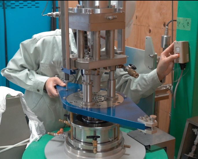

    

    Install loading plate

• V. Shear Box Saturation

  Following the completion of the gap adjustment, the empty shear box is filled with CO₂ and de-aerated water. This procedure is required to prevent air from getting trapped in the shear box, particularly in the gutter. The following steps will describe how to saturate the shear box. Users may also refer to the video tutorial, titled “5. Shear box saturation.”

  • The CO₂ supply comes from the CO₂ tank, which is connected to Valve 05. It is necessary to open a valve at the CO₂ tank up to around 5 and 0.1 MPa (Fig. 27) and then check if CO₂ is going out to every shear box Valve, starting and finishing at Valve 02.

    Fig. 27

    

    Open CO₂ tank

  • The de-aired water supply comes from the vacuum tank connected to Shear box Valve 05. It is necessary to open the air valve at vacuum tank to enable gravity flow and then circulate De-aired water at every shear box Valve, starting and finishing at Valve 02 (Fig. 28).

    Fig. 28

    

    Shear box with the location of the valve

  • When the shear box is filled with de-aired water, close the water supply valve (05) and don’t remove it. Water circulation is needed when the B_d (degree of saturation) value is not high enough. If the water supply is disconnected in this step, air may infiltrate inside the Shear box while reconnecting the water supply. To avoid this, we have to remove the water supply pipe after B_d value check.

  • Install Pore pressure transducers (PPTs) (one to valve 03a, or another one to valve 03b, or both). When PPTs are connected to valves, open PPTs’ drainage valves till a few drops of water come out, then reset u = 0.

  • Remove Loading Plate (valve 02 should be opened during removal of LP from SB).

• VI. Sample setting

  The steps of sample setting are summarized as follows. The reader can also find these steps in the video tutorial titled “6. Sample setting.”

  • Put a filter paper on the bottom of shear box.

  • Slowly built in a sample, and smooth the sample surface. The sample height should be app. 30 mm from the top of the Shear Box (Fig. 29).

    Fig. 29

    

    Smooth the sample surface

  • Put a filter paper on the top of the sample, and tissues if fine-grained material is built in.

  • Before setting of Loading Plate, grease it.

  • Install Loading Plate, with valve (02) opened to enable water drainage. When the position is adjusted (Fixing screws are fitted on holes of LP) push down the system by button. Check Loading Plate position—red marks on FS should be on the LP surface (Fig. 30).

    Fig. 30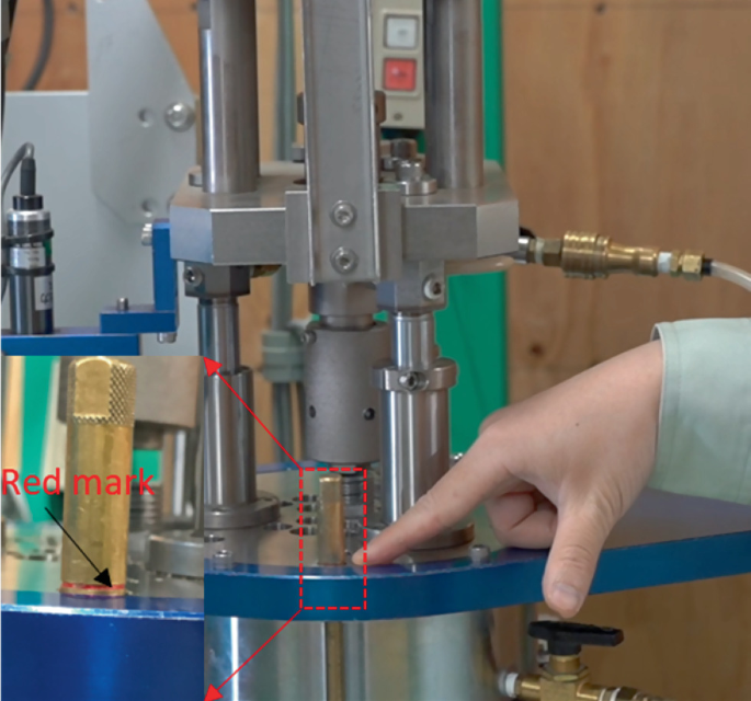

    

    Checking red mark after installation loading plate

  • Put 12 screws on LP but leave them loose.

  • Unscrew and take out Helping screws (3 golden ones).

  • Install Shear Load Cells, and rotate to adjust position (Fig. 31).

    Fig. 31

    

    Adjust the position of loading plate to install shear load cells

  • Install Vertical Load Cylinder (VLC) by controlling on Vertical Control part of MCU (Main Control Unit) (Fig. 32) and check the speed set location. If not 0, turn it to 0 to ensure the central axis does not suddenly move → Click the Down button → Turn the speed set button to 2–4. The VLC goes down and when VLC contacts the central shaft, click the Stop button. Turn the speed set button to 0 and Lock the button.

    Fig. 32

    

    Using vertical control to install vertical load cylinder

  • When VLC contact LP, screw the ring and additionally screw by the screw driver.

  • After LP is fixed, unlock the protection screw on LP.

• VII. Water circulation (gravity flow)

  The de-aired water supply comes from the vacuum tank from which is connected to Shear box Valve 05. It is necessary to open the air valve at vacuum tank to enable gravity flow and then circulate de-aired water though Valve 02. Users may also refer to the video tutorial, titled “7. Water circulation.”

• VIII. B _d value measurement

  B_d is stressed by applying a load in increments of 50 kPa and measuring the generated-pore pressure at two-pore pressure transducers. It must be done in undrained conditions to generate pore water pressure. The B_d value depends on the Rubber Edge Correction Factor (α). The B_d value is calculated based on the following equation.

  $$ {\text{B}}_{{\text{d}}} = \Delta {\text{u}}/\Delta {\text{s}} $$

  where

  Δu is an increment of pore pressure,

  Δσ is an increment of normal stress.

  The loading rate (slope value in kPa/s) depends on soil properties. Slow speeds are recommended for fine-grained materials with low permeability (e.g., for flysch, the slope of 0.1 or 0.25 kPa/s).

  The steps are provided in the video tutorial titled, “8. Bd value”. Here is a summary of the steps:

  • Close the Valve 02.

  • Turn ON the vertical control to manage normal stress.

  • Fill the data form panel for Data acquisition with data appropriate for this specific test and start data acquisition.

  • First, apply 50 kPa, then write u1 or/and u2 values and calculate the Bd value for this loading. Do the same for σ = 100, 150, 200 kPa. Continue to higher stresses if necessary.

  • Calculate the Bd. Bd value should be large 0.95.

  • Stop data acquisition after Bd value measurement is finished.

  • After B_d measurement is finished, we can release normal stress to 0 and then open valve 02 for starting a consolidation process.

• IX. Consolidation

  For each test, sample consolidation is performed to simulate the initial stress condition. In drained conditions, the normal stress and shear stress was raised to a certain value (dependent on sample depth and slope angle). The steps are explained in the instructional videos “9. Consolidations 1” for simulating only normal stress and “10. Consolidations 2” for simulating both shear stress and normal stress, respectively. Here is a brief overview of the steps:

  • Open the Valve 02 (Fig. 33).

    Fig. 33

    

    Open the valve 2 for drainage

  • Enter the data appropriate for this specific test in the data form panel for data acquisition, then start the data acquisition.

  • Calculate and set initial Normal and Shear stresses (σ₀, τ₀) and for the Speed Control test τ₀ = 0. Stress loading speed (kPa/s) depends on material properties”.

  • Consolidation is finished when pore pressure dissipates (u = 0). Close the drainage valve 02 at that time and then stop the data acquisition.

• X. Shearing

Shearing was performed following sample consolidation. It is shareable in both drained and undrained situations. In a condition of drainage, valve 2 is open, but in a state of undrained, it is closed.

A servo-controlled motor provides shear stress via shear stress control, speed control, or displacement control. The choice between a speed control test and a stress control test depends on the test’s objective. Typically, a stress-control test is performed to simulate a landslide, while a speed-control test is utilized to acquire soil characteristics.

• 1. Monotonic shear-stress test (a basic shear stress control test)

  The monotonic shear-stress test is the most fundamental undrained dynamic-loading ring-shear test for measuring the undrained steady-state shear resistance as a key parameter for landslide dynamics. When stress exceeds the failure line, the decrease in shear resistance after peak strength accelerates shear displacement. Increased pore pressure will generate a fast motion during the subsequent post-failure motion. It will continue until it reaches a steady-state shear resistance in an undrained condition. Normally, we set the limit for shear displacement at 10 m. The shearing stops automatically when the shear displacement reaches 10 m.

  The procedures for the monotonic shear-stress test are outlined here, but they are also available in the video instruction titled “11. Shear stress control.”

  • Remove the water supply pipe from Valve 05 and remove all obstacles to the rotation of lower plate (LP).

  • Check again if Helping Rings are unscrewed and removed.

  • Close valve 2 (for the undrained test).

  • Push the remote button in the shear control box (Fig. 34).

    Fig. 34

    

    Pushing the “Remote” button in the Shear control box

  • Click the “Information” button and fill information for Data acquisition (Fig. 35). Select the sampling interval. For the fast speed testing, we often select 5 Hz or 10 Hz for the sampling interval. For slow testing, the users can change the sampling interval to 1 s or higher.

    Fig. 35

    

    Screenshot of setting data acquisition

  • In the shear stress control of the software (Fig. 36), select the shear stress control and click “On” button.

    Fig. 36

    

    Screenshot of setting stress control test

  • Input the parameters: target and slope for the static loading. The slope should be small, such as 0.5 kPa/s, or smaller for fine-grained material with low permeability.

  • Click the “Start” button in the Data acquisition.

  • Click the “Static” button (Fig. 36) to increase shear stress.

  • Click the “Stop” button in the Data acquisition when shearing is finished.

  • Chose the “Measure” button in the Data acquisition to reset the shear displacement to 0. This step is needed because when shear displacement reaches 10 m, the program stops controlling the system.

• 2. Shear-displacement control test or shear speed control test

  Shear stresses at the steady-state, the mobilized and peak friction angles may be determined by conducting an undrained shear displacement control or speed control test. For ICL-2, the maximum speed of the sheared servo-motor is 50 cm/s. A speed test can be conducted in cm/s, whereas a displacement test can be performed in mm/s, mm/min, and mm/h. Fine-grained materials with low permeability should be sheared at a slow speed to see pore pressure build up slowly. A shear-displacement control test is used for very slow shearing tests to test clayey soils for reactivated landslides.

  The steps for the shear-displacement control test are presented here, but they are also available in the video instruction titled “12. Shear displacement control”.

  • Disconnect the water supply pipe from Valve 05 and remove all obstacles to the rotation of lower plate (LP).

  • Verify that the Helping Rings have been unscrewed and removed.

  • Close valve 2 (for the undrained test).

  • Press the “remote” button in the shear control box.

  • Fill out the details for data acquisition by clicking the “Information” button. Select the sampling interval that ranges from 600 s to 200 Hz. Sample intervals of 5 Hz or 10 Hz are frequently chosen for testing at high speeds. Users can adjust the sample interval to 1 s or higher for slow speed.

  • Select the shear displacement control and click “On” in the program (Fig. 37).

    Fig. 37

    

    Screenshot of setting shear displacement control test

  • Enter the target and slope parameters for the static loading. Figure 37 shows an example with a target of 1000 mm and a slope of 0.05 mm. The test takes about 5.6 h.

  • Click the “start” button in the data acquisition.

  • Click the “static” (Fig. 37) to start shearing.

  • Click the “Stop” button in the Data acquisition when shearing is finished.

  The steps for the speed control test are similar to the shear-displacement control test. The difference is the setting of the loading parameters. Figure 38 presents an example of a speed control test. The “target” is the shear speed in cm/s and constant during the test. The “slope” is the time required to get constant shear velocity.

  Fig. 38

  

  Screenshot of setting speed control test and graph illustrating the slope required to achieve constant shear speed

• 3. Cyclic-loading shear-stress control test

  The cyclic shear stress is the fundamental preliminary investigation of the behavior of earthquake-induced landslides. Before performing cyclic loading, the initial stress conditions (σ₀ and τ₀) must be calculated based on the depth of the sample and slope angle. In this example test, we selected normal stress of 1000 kPa and shear stress of 700 kPa. Normal and shear loads are applied in static mode and under drained conditions. The consolidation step is following the instructions in the video titled, “10. Consolidation 2”.

  The video tutorial titled, “13. Cyclic shear control,” explains the procedure, which is also summarized below:

  • Disconnect water supply pipe from Valve 05 and remove all obstacles to rotation of lower plate (LP).

  • Verify that the Helping Rings have been unscrewed and removed.

  • Close valve 2 (for the undrained test).

  • Press the “remote” button in the shear control box.

  • Click the “Information” button and fill in the information for Data acquisition. Select the sampling interval. For cyclic testing, we often select the sampling interval of 5 Hz or 10 Hz.

  • Select the shear stress control and click “On” in the program (Fig. 39).

    Fig. 39

    

    Screenshot of setting and graph illustrating time and shear stress applied for cyclic loading of shear stress

  • Enter the cyclic loading parameters: Initial amplitude, amplification factor, attenuation factor, cycle rate, and phase, number of amplification cycles, number of constant cycles and number of attenuation cycles, period and number of cycles. The cycle rate chosen will depend on the soil’s characteristics. For fine-grained materials, loading at a slow speed (cycle/hour) is preferred, but for coarse-grained materials, a higher rate (cycle/min or cycle/s) can be used. The maximum cyclic shear load is computed using the formula:

    $$ \tau_{\max } = \tau_{0} + \Delta \tau_{im} + (N_{ac} - 1) \cdot \Delta \tau_{af} $$

  where,

  τ_max is the maximum applied shear stress,

  τ₀ is the initial shear stress,

  N_ac is the number of amplification cycles,

  ∆τ_af is the amplification factor

  ∆τ_im is the initial amplitude

  From the setting in Fig. 39, cyclic loading parameters are below:

  • τ₀ = 700 kPa,

  • N_ac = 6,

  • ∆τ_af = 30 kPa/cycle,

  • ∆τ_im = 50 kPa.

  Then, the maximum applied shear stress is as follows: $\tau_{\max } = 700 + 50 + (6 - 1).30 = 900\,{\text{kPa}}$.

  • Click the “start” button in the data acquisition.

  • Click the “cyclic” (Fig. 39) to start shearing.

  • Click the “Stop” button in the Data acquisition when shearing is finished.

  • Chose the “Measure” button in the Data acquisition to reset the shear displacement to 0.

• 4. Pore-water pressure control test—Rain-induced landslide simulation test

  Numerous landslides are triggered by rainfall that can be simulated using ring shear apparatus. The sample was saturated, and then consolidated to initial stresses (σ₀ and τ₀) in a drained condition. This preparatory stage was to reproduce the initial stress on the slope. The pore pressure is gradually increased to simulate the rise in groundwater level during rainfall. The groundwater level rise on natural slopes may not be quick; hence the pore-water pressure loading in a drained condition. When shearing start, we can test under drained or undrained condition. The steps are detailed in the video instruction titled “14. Pore-water pressure control,” with a summary of the steps below.

  • Disconnect water supply pipe from Valve 05 and remove all obstacles to rotation of lower plate (LP).

  • Verify that the Helping Rings have been unscrewed and removed.

  • Close the valve 2.

  • Connect the water pipe to the servo pore water pressure (Fig. 40).

    Fig. 40

    

    Connecting the water pipe to the servo pore water pressure

  • Open the valve in the servo pore water pressure. Push the “loading” button and rotate the “speed set” in the pore water pressure to check the water coming out from the piston of the servo pore water pressure through the water pipe (Fig. 41).

    Fig. 41

    

    Checking water coming out from the piston of servo pore water pressure

  • Connect the water pipe to the valve 4.

  • Push the “stop” and then “remote” buttons to change manual to remote control

  • Fill out the details for data acquisition by clicking the “Information” button. A sample interval of 5 Hz is frequently chosen for the pore water pressure control test.

  • Enter the target and slope parameters for the static loading of pore water pressure.

  • Click the “start” button in the data acquisition.

  • Click the “static” (Fig. 42) to start increasing the pore water pressure.

    Fig. 42

    

    Screenshot of setting pore water pressure control test

  • If we want to test in the undrained shearing, we need to close valve 4 when the lower shear box is rotating.

  • Click the “Stop” button in the Data acquisition when shearing is finished.

  • Chose the “Measure” button in the Data acquisition to reset the shear displacement to 0.

  • Connect the water pipe to the water tank. Then, push the “Return” button to fill out the water to the piston of the servo pore water pressure, until the water comes out from the hole at the center of the piston (Fig. 43).

    Fig. 43

    

    Fill back the water into the piston

  • Push the “stop” button in Fig. 42 and disconnect the water pipe.

• 5. Seismic Test—Earthquake-induced landslide simulation test

  To simulate an earthquake-induced landslide, we will input a shear-stress curve calculated from the real earthquake record or a past earthquake record in the computer.

  When an earthquake occurs and a seismic acceleration is applied, the loaded stress is given as k ⋅ m ⋅ g; k is referred to as the seismic coefficient, which is the ratio of the seismic acceleration (a) and gravity (g), namely k = a/g. It can be used as the control signal for both normal stress and shear stress servo-motors. However, we often examine soils when they are completely saturated. In this instance, the change in normal stress will be negated by the creation of extra pore pressure, and the effective normal stress will be minimal. Then, during the earthquake-induced landslide simulation test, the seismic shear-stress variation is typically inputted while the total normal stress remains constant.

  The additional shear load is simplified and computed using the following formula:

  $$ \Delta \tau_{s} = k \cdot m \cdot g = k \cdot \frac{{\tau_{0} }}{{\sin\theta }} = \frac{{a \cdot \tau_{0} }}{g \cdot \sin \theta } $$

  where,

  ∆τ_s is the additional shear stress due to seismic waves,

  τ₀ is the initial shear stress, τ₀ = m ⋅ g ⋅ sin θ,

  a is the seismic acceleration,

  g: gravity.

  In this manual, the test was consolidated to the normal stress of 400 kPa and shear stress of 300 kPa to create the initial state. The additional shear load was calculated based on the EW component of the 2016 Kumamoto earthquake wave, which caused many of the landslides in the Kumamoto area. The test was conducted at a five-times slower rate to monitor pore water pressure accurately.

  The steps to conduct the seismic test are provided below and in the video titled, “15. Seismic test.”

  • Disconnect the water supply pipe from Valve 05 and remove all obstacles to the rotation of lower plate (LP).

  • Verify that the Helping Rings have been unscrewed and removed.

  • Close the valve 2 (for the undrained test).

  • Fill out the details for data acquisition by clicking the “Information” button. A sample interval of 5 Hz or higher is frequently selected for the seismic tests.

  • Read the wave data by clicking the “File” menu in the Toolbar, and selecting the “Read wave data (R)” option. Next, click on the “opening file icon” to select the text file in the testing computer that contains the wave data. It is noted that the text file containing the wave data should be in a CSV or excel format.

  • Input the parameters for wave data (Fig. 44). The recorded seismic waves contain waves with high frequencies and, at times, great accelerations. The shearing servo motor cannot repeat the high acceleration and loading frequency. Due to constraints, the scale factor and output intervals are used to adjust the actual seismic data. To protect the shear motor and precisely monitor the pore water pressure, we selected an “output interval” of 0.05 s, which is five times lower than the sampling rate of the seismic waves, 0.01 s, that were recorded. In the “Shear stress or Shear displacement data,” select Colum 1, which contains the shear stress or shear displacement, then choose “stress” for the data type and “kPa” for the unit of data.

    Fig. 44

    

    Screenshot of setting the parameters for the input of wave data and preview of imported seismic shear stress in the software

  • Click the “start” button in the data acquisition.

  • Click the “wave” in the shear stress control (Fig. 44) to start seismic stress acting on the sample.

  • Click the “Stop” button in the Data acquisition when shearing is finished.

  • Chose the “Measure” button in the Data acquisition to reset the shear displacement to 0.

• XI. De-installation

  After completing the ring shear test, it is essential to remove and clean all apparatus components meticulously to prevent damage. The steps of de-installation and cleaning are provided below and in the video titled, “16. De-installation.”

  • Release normal and shear stresses to 0 by computer control. Enter “0” in the target and 3–5 in the slope for the static loading parameters of both normal stress and shear stress. Click the “static” buttons in both normal stress and shear stress control. When stresses equal to 0, click the “off” buttons to stop controlling the stresses.

  • Push the “remote” buttons in the main control unit to stop the remote control.

  • Put Helping Screws (3 × golden ones) before removing Loading Plate

  • Disconnect pore water pressure sensors and Shear Load Cells.

  • Uninstall Vertical Load Cylinder (VLC) by Vertical Control part of MCU (Main Control Unit): Unscrew the ring connecting VLC and the loading plate. Check the speed set location. If not 0, turn it to 0 to ensure the central axis does not suddenly move → Click the Down button → Turn the speed set button to 2–4. The vertical displacement decrease and when it is around 0 → Stop → Lock the protection button → Click Up button → the speed set also 2–4, the central axis goes up until around marker → Stop → Turn the speed set button to 0.

  • Unlock the Lifter and connect with VLC.

  • Pull up the loading plate and put it back in to the neutral position.

  • Remove sample, filter paper, and tissues.

  • Remove and clean the inner and outer rings.

  • Clean the rubber edge carefully using acetone to remove Teflon and silicone grease.

  • Decrease Gap to 0 and then Push Gap Off.

  • Turn off shear, gap, vertical, and pore water motors.

  • Turn off the main control unit and computer (Fig. 45).

    Fig. 45

    

    Disconnecting the central axis and loading plate

• XII. Data analysis

  The ring shear program records all measurable data from experiments. The output file (DAT file) contains sensor and test values. The data analysis utilizes only the test value using Excel or other software. To obtain accurate shear stress values, it is necessary to correct two effects of the rubber edge on shear stress and normal stress.

  Granular materials, such as sand cannot sustain cohesiveness after a considerable shear displacement. This assumption holds for sands and other typical soils. This assumption is utilized for normal stress adjustment.

  The ICL-2 has a feature for inputting the normal stress correction factor into the normal stress control system. Figure 46a shows the original stress path result from an undrained cyclic shear stress control test. In the test, we selected a rubber edge correction factor of 0.9. At zero normal stress, the extension of the stress path passes the negative shear stress. When we apply the rubber edge correction factor of 0.86, normal stress equals 1000 * 0.86/0.9 = 955.6 kPa. The shape of the stress path is not changed but moved horizontally to the left. Based on the result in Fig. 18, the correction of rubber edge friction was lowered by 15 kPa from the graph in Fig. 46a. After the corrections of the rubber edge effects, the final stress path result is presented in Fig. 46b.

  Fig. 46

  

  Test result of the undrained cyclic shear-stress control test. Original test data (a) and the correction of rubber edge effects (b)

  After data correction, the test result is displayed in the three relationships below.

  • A time series of data (normal stress, pore water pressure, shear stress, and shear displacement) to examine the process of shearing.

  • A stress path (relationship between the total normal stress and effective stress and shear stress) to understand the dynamic behavior of the sample.

  • A relationship between shear stress and shear displacement. Evaluating the drop in shear stress following a failure to steady-state is essential. When the shear displacement from the failure to the steady-state is short, and the loss in strength from the peak to the steady-state is significant, progressive failure development is quick.

• 1. Monotonic shear-stress test results

  Figure 47 is a monotonic shear stress test result. This test was conducted under normal stress of 500 kPa. From this result, we can obtain friction angle at peak (φ_p = 43.1°), mobilized friction angle at failure (φ_m = 36.4°), steady state shear resistance (τ_ss = 50 kPa), shear displacement at the start of strength reduction (DL = 6 mm) and shear displacement at the start of steady state (DU = 700 mm).

  Fig. 47

  

  Example data of a monotonic increasing shear-stress test. a Time series of data, b stress path, c shear stress and shear displacement relationships. Test conditions: sample: weathered granite soil, BD = 0.95, normal stress = 500 kPa, shear stress increment rate: 0.5 kPa/s

• 2. Shear-displacement control test or shear speed control test

  Figure 48 is a shear-displacement control test result. The silica sand no. 4 was tested under normal stress of 1000 kPa and shear displacement increment rate of 0.05 mm/s. From this result, we can obtain friction angle at peak (φ_p = 37.2°), mobilized friction angle at failure (φ_m = 37.2°), steady state shear resistance (τ_ss = 215 kPa), shear displacement at the start of strength reduction (DL = 6 mm) and shear displacement at the start of steady state (DU = 102 mm).

  Fig. 48

  

  Example data of a shear-displacement control test. a Time series of data, b stress path, c shear stress and shear displacement relationships. Test conditions: sample: silica sand no. 4, BD = 0.97, normal stress = 1000 kPa, shear displacement increment rate: 0.05 mm/s

• 3. Cyclic-loading shear-stress control test

  Figure 49 displays the results of the undrained cyclic test. The green line represents the shear-stress control signal applied to the stress-control servo-motor, while the red line represents the mobilized shear resistance. The control signal for shear stress and the mobilized shear resistance are at the same level in the beginning state. When soil collapse takes place, these two lines diverge. In line with the prescribed cyclic loading, the control signal rises as the shear resistance falls until a steady-state shear resistance that is less than the starting stress equivalent to the stress due to gravity. We can determine friction angle at peak (φ_p = 38.8°), mobilized friction angle at failure (φ_m = 35.9°), steady state shear resistance (τ_ss = 55 kPa), shear displacement at the start of strength reduction (DL = 100 mm) and shear displacement at the start of steady state (DU = 700 mm).

  Fig. 49

  

  Example data of a cyclic-loading shear-stress control test. a Time series of data, b stress path, c shear stress and shear displacement relationships. Test conditions: sample: silica sand no. 4, BD = 0.97, normal stress = 945 kPa, shear stress = 670 kPa, cyclic rate: 0.5 cycle/s, shear stress step = 30 kPa

• 4. Pore-water pressure control test—Rain-induced landslide simulation test

  The undrained loading condition was not applied because, on natural slopes, the increase in groundwater level may not occur quickly. The pore water pressure is supplied to the shear box from the piston of the pore water pressure control through valve 4 and then the natural drained condition is applied to the sample. After failure, the test condition can change from drained to undrained by closing valve 4. As shown in Fig. 50, failure occurred at pore-water pressure of 50 kPa, that is pore-water pressure ratio r_u = 50/400 = 0.125.

  Fig. 50

  

  Example data of a pore-water pressure control test-test. a Time series of data, b stress path. Test conditions: sample: silica sand no. 4, BD = 0.96, normal stress = 400 kPa, shear stress = 280 kPa, pore-water pressure rate = 1 kPa/s

• 5. Seismic Test—Earthquake-induced landslide simulation test

  Figure 51 presents the test results of the undrained dynamic-loading ring-shear test on the silica sand no.6 using seismic shear stress of the 2016 Kumamoto earthquake wave. Pore pressure was generated during the seismic loading and the stress path reached the failure line. We can determine friction angle at peak (φ_p = 39.1°), mobilized friction angle at failure (φ_m = 36.4°), steady state shear resistance (τ_ss = 40 kPa), shear displacement at the start of strength reduction (DL = 20 mm) and shear displacement at the start of steady state (DU = 700 mm).

  Fig. 51

  

  Example data of a cyclic-loading shear-stress control test. a Time series of data, b stress path, c shear stress and shear displacement relationships. Test conditions: sample: silica sand no. 4, BD = 0.95, normal stress = 400 kPa, shear stress = 280 kPa, seismic wave: 2016 Kumamoto earthquake, five-time lower speed

7 Chapter 5: Conclusions

Sassa and his colleagues at ICL have invented and developed the ICL-1 and ICL-2 ring-shear apparatus series. Several safety protocols have been designed for ICL-2 to reduce any misuse-related harm to the equipment. The concept, design, and construction of the latest ring-shear apparatus, ICL-2, were introduced in this paper.

This article provided a comprehensive guide for interested people to rapidly and effectively operate the ring shear equipment. The user manual supplied in this article was complemented with video demonstrations visually representing each testing phase. In addition to presenting data analysis, the paper provides five basic test cases. Specifically, conventional silica sand no. 4 was tested using the 2016 Kumamoto earthquake wave, which caused many landslides.

Appendix: Test Check List

References

Bishop AW, Green GE, Garga VK, Andersen A, Brown JD (1971) A new ring shear apparatus and its application to the measurement of residual strength. Géotechnique 21(1):273–328
Bromhead EN (1979) A simple ring shear apparatus. Ground Eng 12(5):40–44
Garga V, Infante Sedano JA (2002) Steady state strength of sands in a constant volume ring shear apparatus. Geotech Test J 25(4):414–421
Hungr O, Morgenstern NR (1984) High velocity ring shear tests on sand. Géotechnique 34(3):415–421
Savage SB, Sayed M (1984) Stresses developed in dry cohesionless granular materials sheared in an annular shear cell. J Fluid Mech 142:391–430
Sassa K (1984) The mechanism starting liquefied landslides and debris flows. In: Proceedings of 4th international symposium on landslides, Toronto, June, pp 349–354
Sassa K (1992) Access to the dynamics of landslides during earthquakes by a new cyclic loading high-speed ring-shear apparatus (keynote paper). In: 6th international symposium on landslides, “Landslides”, A.A. Balkema, Christchurch, 10–14 Feb, vol 3, pp 1919–1937
Sassa K (1997) A new intelligent-type dynamic-loading ring-shear apparatus. Landslide News 10:33
Sassa K, Fukuoka H, Wang G, Ishikawa N (2004) Undrained dynamic-loading ring-shear apparatus and its application to landslide dynamics. Landslides 1(1):7–19
Sassa K, He B, Miyagi T, Strasser M, Konagai K, Ostric M, Setiawan H, Takara K, Nagai O, Yamashiki Y, Tutumi Y (2012) A hypothesis of the Senoumi submarine megaslide in Suruga Bay in Japan—based on the undrained dynamic-loading ring shear tests and computer simulation. Landslides 9(4):439–455
Sassa K, Dang K, He B et al (2014) A new high-stress undrained ring-shear apparatus and its application to the 1792 Unzen–Mayuyama megaslide in Japan. Landslides 11:827–842. https://doi.org/10.1007/s10346-014-0501-1
Sassa, K., Dang, K. (2018) Text tool 0.081-1.1 landslide dynamics for risk assessment. In: Sassa K, Tiwari B, Liu K, McSaveney M, Strom A, Setiawan H (eds) Landslide dynamics-ISDR-ICL landslide interactive teaching tools. Springer, pp 1–79
Setiawan H, Sassa K, He B (2018) TXT-tool 3.081-1.6: manual for undrained dynamic-loading ring shear apparatus. In: Sassa K et al (eds) Landslide dynamics: ISDR-ICL landslide interactive teaching tools, vol. 2: testing, risk management and country practices. Springer, Cham, pp 321–350. https://doi.org/10.1007/978-3-319-57777-7_18
Tika TM (1989) The effect of rate of shear on the residual strength of soil. PhD Thesis, University of London (Imperial College of Science and Technology), 494p
Acknowledgements
The authors gratefully acknowledge funding from a Japan-Sri Lanka bilateral SATREPS (Science and Technology Research Partnership for Sustainable Development) project titled “Development of early warning technology of Rain-induced Rapid and Long-traveling Landslides joint program from 2019–2025.” The International Consortium on Landslides (ICL) and the National Building Research Organization of Sri Lanka (NBRO) are implementing this project.
Author information
Authors and Affiliations
Editor information
Editors and Affiliations
1 Electronic supplementary material
Below is the link to the electronic supplementary material.
1. Sample saturation and water preparation
2. Preparing the sample mold
3. Switching on the Ring shear apparatus
4. Gap adjustment
5. Shear box saturation
6.Sample setting
7. Water circulation
8. Bd value
9. Consolidations 1” for simulating only normal stress
10. Consolidations 2” for simulating both shear stress and normal stress
11. Shear stress control
12. Shear displacement control