Spin Dynamics

Abstract

This chapter is a general introduction to spin dynamics in beam lines and accelerators, and to resonant depolarization in cyclic accelerators.

A Gérard Leleux

This manuscript has been authored by Brookhaven Science Associates, LLC under Contract No. DE-SC0012704 with the U.S. Department of Energy. The United States Government and the publisher, by accepting the article for publication, acknowledges that the United States Government retains a non-exclusive, paid-up, irrevocable, world-wide license to publish or reproduce the published form of this manuscript, or allow others to do so, for United States Government purposes.

2.1 Introduction

This lecture is largely based on various of the founding theoretical papers and earlier lectures regarding spin dynamics in cyclic accelerators, including, especially, Saturne 1970s–1990s reports and lectures by Gérard Leleux et al. [1,2,3,4,5], theoretical work at the ZGS [6], and Courant and Ruth’s 1980 BNL report [7].

Documentation used includes in addition the milestone articles by Thomas [8], Bargman et al. [9], Froissart and Stora [10], L.C. Teng [11], Montague [12], as well as reviews by Buon and Koutchouk [13], S. Mane et al. [14], and textbooks by S.Y. Lee [15], and Conte and MacKay [16].

This list, although substantial, is far from exhaustive, however it is believed to be a sound starting point for further exploration and advanced knowledge, beyond the present brief theoretical introduction to spin dynamics and depolarizing resonances.

2.2 Spin Precession

2.2.1 Magnetic Moment of a Spinning Charge

Consider a mass with uniform density, spinning around its center of mass: ρ_m = m∕V ; its spin angular momentum can be written

$$\displaystyle \begin{aligned} \mathbf S = \dfrac{m}{V} \int \mathbf r \times \mathbf v (\mathbf r) d^3r \end{aligned} $$

(2.1)

Assuming this volume uniformly charged, with density ρ_q = q∕V , the resulting magnetic dipole moment reads

$$\displaystyle \begin{aligned} \mathbf \mu = \dfrac{q}{2V} \int \mathbf r \times \mathbf v (\mathbf r) d^3r \end{aligned} $$

(2.2)

In this model, spin angular momentum S and resulting magnetic moment μ are colinear vectors and satisfy

$$\displaystyle \begin{aligned} \mathbf \mu = \dfrac{q}{2m} \, \mathbf S \end{aligned} $$

(2.3)

2.2.2 Spin Precession

If a magnetic dipole μ is dipped in a magnetic field B, it undergoes a torque

$$\displaystyle \begin{aligned} \boldsymbol \tau = \mathbf \mu \times \mathbf B \end{aligned} $$

(2.4)

This torque exerted by B causes μ, or equivalently its spin angular momentum S, to precess around B. The rate of change of the angular momentum is

$$\displaystyle \begin{aligned} \boldsymbol \tau \equiv \dfrac{d\mathbf S}{dt } = \underbrace{g\, \dfrac{q}{2m}\, \mathbf S}_{\text{equivalent } \boldsymbol \mu }\! \! \times\, \mathbf B \ =\mathbf S \times \boldsymbol \Omega \end{aligned} $$

(2.5)

$g=\dfrac {2m}{q}\dfrac {\mu }{S}$ is the Landé factor, or gyromagnetic ratio. It takes the value g = 2 for a point particle. Note that Sect. 2.2 model for $\dfrac {\mu }{S}$ isn’t that far, a factor ≈2 away (Eq. 2.3; Fig. 2.1).

Fig. 2.1

A sketch of a torque effect in a current loop model. Assume μ due to a current loop: the change in angular momentum is the direction of the torque, i.e. sideways. The torque expresses as $\boldsymbol {\tau } = \int \mathbf {r} \times d \mathbf {F} = \int \mathbf {r} \times (\mathbf {v} \times \mathbf {B}) dq = \boldsymbol {\mu } \times \mathbf {B}$

Introduce the quantity $a = \dfrac {g-2}{2}$, the gyromagnetic anomaly, a measure of the departure of g from 2 (usually noted a for leptons, G for hadrons). It takes the following values, for diverse particles:

$$\displaystyle \begin{aligned} \underbrace{ 1.159652\times 10^{-3}}_{\mathrm{electron}}, \quad \underbrace{ 1.165921\times 10^{-3}}_{\mathrm{muon}}, \quad \underbrace{ 1.792847 }_{\mathrm{proton }}, \quad \underbrace{ -4.184153 }_{\mathrm{helion}}, \quad \underbrace{ -0.14301 }_{\mathrm{deuteron}} \end{aligned} $$

(2.6)

2.2.3 Thomas-BMT Equation of Motion

In accelerators and beam lines particles move in the fields of guiding, focusing and accelerating systems. These laboratory fields Lorentz-transform into a magnetic component B_com in the particle frame (the electric component is ignored here, as it does not couple to the magnetic moment). A torque results, which writes

$$\displaystyle \begin{aligned} \dfrac{d\mathbf S}{dt } \equiv \mathbf \tau = (1+G) \dfrac{q}{m} \mathbf S \times \mathbf B_{\mathrm{com}} \end{aligned} $$

(2.7)

Expressing B_com in terms of the Lorentz transformed laboratory fields B and E (note that E contributes to B_com) yields the Thomas-BMT equation of spin motion in the laboratory frame [9]

$$\displaystyle \begin{aligned} \dfrac{d\mathbf S}{dt} = \dfrac{q}{\gamma m}\mathbf S \times \left[ (1+G\gamma)\mathbf B_{\perp} +(1+G)\mathbf B_{\parallel} + \left( \dfrac{1}{\gamma +1} +G \right)\gamma \dfrac{\mathbf E \times \boldsymbol \beta}{c} \right] {} \end{aligned} $$

(2.8)

wherein

• S(t) is taken in the particle frame, it has not been Lorentz-transformed,

• all other quantities, including time, are expressed in laboratory frame,

• B_∥∥v and B_⊥ = B −B_∥ field components have been introduced.

Note that, from the expressions above it results that $\mathbf S \cdot \dfrac {d\mathbf S}{dt} = 0$, which establishes that |S|=constant.

Two Comments

• 1. In the combined torque

  $$\displaystyle \begin{aligned} \dfrac{d\mathbf S}{dt} = \dfrac{q}{\gamma m}\mathbf S \times \Big[ \underbrace{(1+G\gamma)\mathbf B_{\perp} +(1+G)\mathbf B_{\parallel}}_{ \approx G\gamma B} + \underbrace{\left( \dfrac{1}{\gamma +1} +G \right) \gamma \dfrac{\mathbf E \times \boldsymbol \beta}{c}}_{\approx G\gamma E/c} \Big]\end{aligned}$$

  E ⊥v and B ⊥v components may be of comparable strengths, for instance in beam optics conditions where B ≈ 100 Gauss and E ≈ MV/m.

  However, electric fields from accelerating RF cavities in circular accelerators are parallel to v, thus |E ×v| is small. They may usually be ignored, such will be the case in studying depolarizing resonances in next sections.

• 2. Orbit perturbation by the magnetic moment of the particle will be ignored in the remainder of this chapter, the effect is negligible at energies of concern in accelerators. However, this is the origin of the Stern-Gerlach effect.

  The Stern-Gerlach experiment (performed 3 years before Uhlenbeck and Goudsmit hypothesis of the spinning electron) proved that (“Bohr-Sommerfeld hypothesis”) the direction of the angular momentum of atoms is quantized:

  • silver atoms travel through a region of non-uniform magnetic field,

  • the atoms are deflected as they experience a force

    $$\displaystyle \begin{aligned} \mathbf F = \dfrac{d\mathbf p}{dt} = \boldsymbol \mu \cdot \mathbf{grad}\,\mathbf B\end{aligned}$$

    which stems from the non-uniform interaction (a differential effect) of the magnetic dipole with the field,

  • deflections appear to be in two discrete directions (up and down, in the experiment), they do not yield a continuum of atom distribution in space (as would result from a continuum of magnetic moment orientations).

  This deflection property by a non-uniform field allows guiding (using quadrupole fields) and focusing (using sextupole fields) of slow neutron beams (fermions with ±ħ∕2 spin) along beam lines.

Example 1: Spin Precession Through a Dipole Magnet

In the laboratory frame, the spin vector precesses by an angle

$$\displaystyle \begin{aligned} \phi_{\mathrm{sp,Lab}} = (1+G\gamma) \ \times \!\! \overset{\overset{\overset{\text{trajectory}}{\text{deviation}}}{\downarrow}}{\alpha}\end{aligned}$$

while the velocity vector precesses an angle α.

In the moving frame, spin precession amounts to

$$\displaystyle \begin{aligned} \phi_{\text{sp, moving frame}} = \ G\gamma \, \alpha.\end{aligned}$$

Example 2: A Proton Orbiting in the Uniform Field of a Cyclotron Magnet

“Much of the physics of spin motion can be illustrated using the simplest model of a storage ring consisting of uniform horizontal bending and no straight sections.” [ 12 ].

The case of a 200 keV proton, γ = 1.000213, orbiting in the (X_Lab, Y_Lab) plane is illustrated in Fig. 2.2. The number of spin precessions per turn amounts to

$$\displaystyle \begin{aligned} 1+G\gamma = 1+1.793229\end{aligned}$$

Fig. 2.2

A proton is circling (solid line in the (X_Lab, Y_Lab) plane) in a uniform field normal to the orbit. The vector attached to the proton and pointing towards the (X_Lab.Y_Lab)-normal represents its spin, observed here in the moving frame. The magnitude of the spin component normal to the orbit is given on the S_Z axis

in the laboratory frame.

By analogy with the betatron tune, the number of spin precessions per turn is the

$$\displaystyle \begin{aligned} \text{spin tune:} \quad u_{\mathrm{sp}} = \dfrac{\omega_{\mathrm{prec}} - \omega_{\mathrm{rev}} }{\omega_{\mathrm{rev}}} =G\gamma\end{aligned}$$

a quantity defined in the moving frame.

In Fig. 2.3 spin motion is observed in the moving frame, the figure shows the projection of the spin vector in the bend plane, in the case of an integer or fractional Gγ value.

Fig. 2.3

Case of a proton orbiting in a uniform field, projection of the spin vector in the bend plane, along the proton orbit, in the case of an integer or fractional Gγ value. (a) Case of an integer number of spin precessions over a turn: ν_sp = Gγ = 2 here, spin motion closes on itself after a turn. (b) Case of a fractional number of spin precessions over a turn: ν_sp = Gγ = 1.7932 here, spin motion starts at about 2 o’clock, it does not close after a turn

These basic aspects of spin motion are further exemplified in Sect. 2.4, as follows:

• Exercise 1, which deals with a low energy spin rotator based on a Wien filter; theoretical parameters are derived and applied in a numerical simulation of the device;

• Exercise 2, which investigates spin motion in a uniform magnetic field, and provides a hint at resonant spin motion, under the effect of the perturbative torque from a field defect in an otherwise uniform magnetic field; proper parameters for resonance are determined and used in spin tracking simulations;

• Exercise 3, a series of simulations which introduce to, and play with, periodic spin closed orbit and stable spin precession direction in a cyclic accelerator.

2.3 Depolarizing Resonances in Cyclic Accelerators

In the bending magnets of a planar cyclic accelerator, spins precess around the vertical axis at a frequency Ω_sp. There is no precession in drift spaces, the orientation of the spin vector remains unchanged. In the perturbing fields resulting for instance from off mid-plane motion at main bend extremities ($B_s= \dfrac {\partial B_y}{\partial s}y$), or in quadrupole fields (B_x ∝ y), spins precess around a local non-vertical axis, with a related frequency Ω_pert.. If the two frequencies Ω_sp and Ω_pert. get close to one another, the average precession axis moves away from the vertical, the more so as perturbative fields are stronger, and this results in beam depolarization. The dynamics of resonant depolarization is studied with some detail in this Section, which owes much to Ref. [3].

2.3.1 Polarization

A beam is a set of particles, polarization of a ±½ spin particle beam is defined as the statistical average

$$\displaystyle \begin{aligned} \overline P = \dfrac{n^{\uparrow}-n^{\downarrow}}{n^{\uparrow} + n^{\downarrow}}\end{aligned}$$

with $n^{{ }^{\uparrow \downarrow }}$ the number of particles with spin “up” or “down”, corresponding to the eigenstates ±ħ∕2.

The average polarization behaves as a classical quantity, a spin 3-vector S, of which the evolution is

• determined by a torque applying on the magnetic moment associated with the spin angular momentum,

• and described by the Thomas-BMT equation.

This is the principle of correspondence: “the expectation value of the vector operator representing the ‘spin’ will necessarily follow the same time dependence as one would obtain from a classical equation of motion.” [9].

Spin 1 particles—deuteron for instance—have three eigenstates + ħ, 0,  −ħ. The polarization is the statistical average

$$\displaystyle \begin{aligned} \overline P = \dfrac{n^{\uparrow}-n^{\downarrow}}{n^{\uparrow} + n_0 + n^{\downarrow}}\end{aligned}$$

and follows the classical equation of spin motion. General considerations regarding spin transport in relation with accelerator design can be found in Ref. [16].

2.3.2 Perturbing (Depolarizing) Fields

As aforementioned, electric fields from accelerating cavities are ignored, as they result in essentially E ∥ v. The differential equation of spin motion (Eq. 2.8) simplifies to

$$\displaystyle \begin{aligned} \dfrac{d\mathbf S}{dt} = \dfrac{q}{\gamma m}\mathbf S \times \left[ (1+G\gamma) \mathbf B_{\perp} +(1+G)\mathbf B_{\parallel} \right] ~ ~ ~ {} \end{aligned} $$

(2.9)

Writing it under the slightly different form

$$\displaystyle \begin{aligned} \dfrac{d\mathbf S}{dt} = \dfrac{q}{\gamma m}\mathbf S \times \left[ \mathbf B + G(\mathbf B_{\parallel} + \gamma \mathbf B_{\perp}) \right] {} \end{aligned} $$

(2.10)

with B = B_⊥ + B_∥ the local field, the origin of depolarization is manifest: assume S essentially vertical and B ∥S, thus B_∥≪ γB_⊥ and

$$\displaystyle \begin{aligned} \dfrac{d\mathbf S}{dt}\propto \mathbf S \times \mathbf B \approx0 \end{aligned}$$

whereas, any angle between B and S causes S to vary, $\dfrac {d\mathbf S}{dt} eq 0$. It can be concluded that depolarization results from transverse field components B_x or B_s.

Equation 2.9 shows in addition that spins S spread out, i.e. beam depolarizes, under the effect of

• beam momentum spread (γ factor in Eq. 2.9);

• betatron motion: a different B_⊥(t) and B_∥(t) history for each particle.

2.3.3 Re-write Thomas-BMT Equation of Motion

Thomas-BMT equation of motion can be written with fields B_∥ and B_⊥ expressed in the moving frame, i.e., in terms of particle coordinates along the accelerator reference orbit, as it is the coordinates we use for particle dynamics in cyclic accelerators.

Start from the differential equation in the laboratory system:

$$\displaystyle \begin{aligned} \dfrac{d\mathbf S}{dt} = \dfrac{q}{\gamma m}\mathbf S \times \left[ (1+G\gamma) \mathbf B_{\perp} +(1+G)\mathbf B_{\parallel} \right] ~ ~ {} \end{aligned} $$

(2.11)

Fields in this equation are defined in the laboratory system (O;η, ξ, y) (Fig. 2.4).

Fig. 2.4

Laboratory frame (O;η, ξ, y) (y axis normal to the (η, ξ) plane) and moving frame (s, x, y). Change of frame from one to the other:

Resort to usual working hypotheses of particle dynamics:

• the moving frame (M₀;s, x, y), Fig. 2.5, is considered, normed, a direct triedra, its origin M₀ is the projection of particle position M(s, x, y) on the reference orbit r₀(s); s is tangent to the reference orbit, x is radial, y is vertical,

  Fig. 2.5

  

  Moving frame

• M₀ is at abscissa s along reference orbit and moves with velocity ds∕dt,

• reference orbit is assumed planar: an arc in bends (local curvature 1∕ρ(s) along the reference orbit), straight line otherwise,

• r(s) = r₀(s)  +  xx  +  yy is the trajectory of M,

• kinematic terms will be developed to first order in x and y,

• longitudinal excursion is ignored, transverse only is considered,

• magnetic field considered is of general form (dipoles and lenses),

  B(s, x, y) = B_ss + B_xx + B_yy, arbitrary order in x, y

Resort to the regular differential elements toolkit of particle dynamics:

• s is defined by $\mathbf s = \dfrac {d\mathbf r_0}{ds}$ thus |dr₀| = ds;

• θ only changes in bends;

• in bends (r, θ, y) forms a cylindrical frame;

• one has dx ∥s,  ds ∥−x;

• $\dfrac {d\mathbf x}{ds} = \dfrac {\mathbf s}{\rho }, \quad \dfrac {d\mathbf s}{ds} = -\dfrac {\mathbf x}{\rho }, \quad \dfrac {d\mathbf y}{ds} =0$;

• in the absence of curvature:

  $$\displaystyle \begin{aligned} \rho \rightarrow \infty, \ \ 1/\rho = 0,\ \ d\mathbf x = d\mathbf s = d\mathbf y = 0, \ \ ds \ \text{ is finite and } d\theta=0;\end{aligned}$$

• develop kinematic terms to first order by virtue of

  $$\displaystyle \begin{aligned} \dfrac{x}{\rho} \ll x' \ll \rho x'' \ll 1; \ \ \dfrac{y}{\rho} \ll y' \ll \rho y'' \ll 1\end{aligned}$$

Express B_∥ and B_⊥ in the Moving Frame

The particle velocity writes

$$\displaystyle \begin{aligned} \mathbf v(s,x,y) = \dfrac{d\mathbf r}{dt}= \dfrac{d\mathbf r}{ds} \dfrac{ds}{dt} = \dfrac{ds}{dt} \left[ \left( 1 + \dfrac{x}{\rho} \right) \mathbf s + \dfrac{dx}{ds} \mathbf x + \dfrac{dy}{ds} \mathbf y \right]\end{aligned}$$

This yields

$$\displaystyle \begin{aligned} \mathbf B_{\parallel} = \dfrac{\mathbf v}{v} \left( \dfrac{\mathbf v}{v} \cdot \mathbf B \right) = \dfrac{ds}{dt} \ \dfrac{\mathbf v}{v^2} \left( \begin{array}{c} 1 + \dfrac{x}{\rho} \\ x' \\ y' \end{array}\right)\cdot \left(\begin{array}{c}B_s\\ B_x\\ B_y \end{array} \right)\end{aligned}$$

From this intermediate result it can be observed that, to the first order in x, y,

$$\displaystyle \begin{aligned} \Bigg\{\hspace{-2pt} \left. \begin{array}{l} \text{quadrupoles do not contribute}\ \mathbf B_{\parallel},\quad \text{as}\quad B_x\propto y, \ B_s=0 , \ B_y\propto x, \\ \text{dipoles do, as } \mathbf B_y = B_0 \mathbf y; \text{their end fields too as } \ \mathbf B_s = B_0\rho_0 \ y \dfrac{\partial(1/\rho)}{\partial s}\mathbf s \ \text{(Fig. 2.6).} \end{array} \right.\end{aligned}$$

Note that $B_s = B_0\rho _0 \ y\dfrac {d(1/\rho )}{ds}$ as used here, results from $\underbrace {\dfrac {\partial B_s}{\partial y} = \dfrac {\partial B_y}{\partial s}\, \dfrac {1}{1+\frac {x}{\rho }}}_{\text{from Maxwell's equations} }\approx \dfrac {\partial B_y}{\partial s} = B_0 \rho _0 \dfrac {\partial }{\partial s} \left ( \dfrac {1 }{\rho } \right )$

Fig. 2.6

End field and off-mid plane B_s component, in a dipole magnet

Writing the scalar product explicitly yields

$$\displaystyle \begin{aligned} \mathbf v\cdot \mathbf B =\dfrac{ds}{dt} \left[ (1+\dfrac{x}{\rho})B_{s} + \dfrac{dx}{ds}B_x+ \dfrac{dy}{ds}B_{y} \right]\end{aligned}$$

$$\displaystyle \begin{aligned} \approx \dfrac{ds}{dt} (1+\dfrac{x}{\rho})\left[ B_{s} + \dfrac{dy}{ds}B_{y} (1-\dfrac{x}{\rho})\right] \approx \dfrac{ds}{dt} (1+\dfrac{x}{\rho}) \left[ B_{s} + \dfrac{dy}{ds}B_{y} \right]\end{aligned}$$

Consistently with the earlier hypothesis of a linear approximation of the equations of motion, drop terms quadratic in x, x’, y’ from $|\mathbf v| = \dfrac {ds}{dt} \left [ \big ( 1 + \dfrac {x}{\rho } \big ) + x^{\prime 2} + y^{\prime 2} \right ]^{1/2}$, thus $\mathbf v = \dfrac {d s}{dt} \left [ \left ( 1 + \dfrac {x}{\rho } \right ) \right ] \mathbf s$, yielding

$$\displaystyle \begin{aligned} \mathbf B_{\parallel} = \dfrac{1}{v^2}\, \mathbf v \, ( \mathbf v \cdot \mathbf B) = \left[ B_{s} + \dfrac{dy}{ds}B_{y} \right] \mathbf s \quad \text{and} \quad \mathbf B_{\perp} =\mathbf B - \mathbf B_{\parallel} = - \dfrac{dy}{ds}B_{y} \mathbf s +B_x \mathbf x + B_y \mathbf y\end{aligned}$$

Substitute B_⊥ and B_∥ in Eq. 2.11, this gives

$$\displaystyle \begin{aligned} \dfrac{d\mathbf S }{ dt} = \dfrac{q }{ \gamma m} \, \mathbf S\times \left[ (1+G) B_{s} \mathbf s + (1+G\gamma )B_x \mathbf x + (1+G\gamma )B_{y} \mathbf y + G(1-\gamma )\dfrac{dy}{ds}B_{y} \mathbf s \right]\end{aligned}$$

Now, back to laboratory coordinates (Fig. 2.4), using

$$\displaystyle \begin{aligned} \left\{ \begin{array}{l} \mathbf s = \boldsymbol \eta \cos \alpha - \boldsymbol \xi \sin \alpha \\ \mathbf x = \boldsymbol \eta \sin \alpha + \boldsymbol \xi \cos \alpha \\ \mathbf y = \mathbf y \end{array} \right.\end{aligned}$$

wherein α(t) represents the precession of the velocity vector and increases in bending magnets following α(t) = βct∕ρ. This mapping yields

(2.12)

or, in projection on the laboratory (η, ξ, y) axes,

$$\displaystyle \begin{aligned} \begin{array}{rcl} \dfrac{d }{ dt}\left( \begin{array}{c} S_{\eta} \\ S_{\xi} \\ S_{y} \end{array} \right) = \dfrac{q }{ m \gamma} \, \mathbf S\times \left( \begin{array}{c} (1+G) B_{s}\cos\alpha + G(1-\gamma )\dfrac{dy}{ds} B_{y} \cos \alpha + (1+G\gamma )B_x\sin \alpha \\ - (1+G) B_{s}\sin\alpha - G(1-\gamma )\dfrac{dy}{ds} B_{y} \sin \alpha + (1+G\gamma )B_x\cos \alpha \\ B_{y} (1+G\gamma ) \end{array} \right) \\ {} \end{array} \end{aligned} $$

(2.13)

Comments

Write the torque cross product:

$$\displaystyle \begin{aligned} \dfrac{d }{ dt}\left( \begin{array}{c} S_{\eta} \\ S_{\xi} \\ S_{y} \end{array} \right) = \dfrac{q }{ m \gamma} \, \left( \begin{array}{c} S_{\eta} \\ S_{\xi} \\ S_{y} \end{array} \right) \times \, \left( \begin{array}{c} \Omega_{\eta} \\ \Omega_{\xi} \\ \Omega_y \end{array} \right) =\dfrac{q }{ m \gamma} \, \left( \begin{array}{c} S_{\xi} \Omega_y- S_y \Omega_{\xi}\\ S_y \Omega_{\eta} - S_{\eta} \Omega_y \\ S_{\eta} \Omega_{\xi}- S_{\xi} \Omega_{\eta} \end{array} \right) \begin{array}{c} \\ \\ \leftarrow \dfrac{\mathrm{dS}_{\mathrm{y}}}{\mathrm{dt}} \end{array} {} \end{aligned} $$

(2.14)

Explicit the components of the precession vector Ω:

$$\displaystyle \begin{aligned} \left\{ \begin{array}{lll} \Omega_{\eta}= (1+G) B_{s}\cos\alpha + G(1-\gamma )\dfrac{dy}{ds} B_{y} \cos \alpha + (1+G\gamma )B_x\sin \alpha && \text{perturbation} \\ \Omega_{\xi} = - (1+G) B_{s}\sin\alpha - G(1-\gamma )\dfrac{dy}{ds} B_{y} \sin \alpha + (1+G\gamma )B_x\cos \alpha && \text{perturbation} \\ \Omega_y = B_{y} (1+G\gamma ) && \text{main component} \end{array} \right. {} \end{aligned} $$

(2.15)

• When considering dipole and quadrupole fields only (B_s = 0):

  • the perturbation (namely, the transverse components: Ω_η and Ω_ξ) only appears if there is vertical motion;

  • quadrupole fields are the main contribution, as B_x = G y results in $\dfrac {d S_y}{dt} = S_{\eta } \Omega _{\xi }- S_{\xi } \Omega _{\eta } eq 0$ (Eq. 2.14). This is however a small quantity as S_η, Ω_ξ, S_ξ and Ω_η all are presumably small quantities, thus the variation of S_y is slow.

    If x=0 then Ω = ( Ω_η, Ω_ξ, 0) ⊥y, i.e., the local precession axis is in the bend plane.

• Assume in addition S ≈S_y as expected in a circular accelerator, namely, dS∕dt ≈ (−S_y Ω_ξ, S_y Ω_η, 0): in dipoles where Ω_y ≫ Ω_η, Ω_ξ, it results that dS∕dt ⊥ Ω_y.

Consider fields along a 1-turn periodic closed orbit in a cyclic accelerator: they are 1-turn periodic, namely, B(α + 2π) = B(α). As a consequence, Ω is 1-turn periodic (Eq. 2.15),

$$\displaystyle \begin{aligned} \boldsymbol \Omega(\alpha + 2\pi ) = \boldsymbol \Omega(\alpha )\end{aligned}$$

thus, Ω(α) describes the stable spin precession axis around the ring.

2.3.4 Integral Form of the Solution S(θ)

First simplify notations, by introducing the projection of $\mathbf S= \left ( \begin {array}{c} S_{\eta } \\ S_{\xi } \\ S_{y} \end {array} \right )$in the bend plane, using the complex notation

$$\displaystyle \begin{aligned} s_{\pi} = S_{\eta} + j S_{\xi} {} \end{aligned} $$

(2.16)

Reducing the expression of the spin to two components is justified as the three coordinates of S are not independent: as the spin vector is normalized to 1, s_π yields the vertical spin component

$$\displaystyle \begin{aligned} S_{y} = \sqrt{1 - |s_{\pi}|{}^2} {} \end{aligned} $$

(2.17)

This allows re-writing the differential equation,

$$\displaystyle \begin{aligned} \dfrac{d s_{\pi} }{ dt} &= \dfrac{q }{ \gamma m} \, \bigg( -j B_{y} (1+G\gamma) s_{\pi} - S_{y} e^{ \textstyle -j\alpha} \\ &\quad \times\left[ -j (1+G) B_{s} + (1+G\gamma )B_x -jG(1-\gamma)\dfrac{dy}{ds} B_{y} \right] \bigg) {} \end{aligned} $$

(2.18)

Introduce the guiding field $B_{y0} =\dfrac { B_0 \rho _0 }{ \rho _0}$, so that

• B_y(θ) = B_y0(θ) +  ΔB_y(θ)

• B_y0 ≠ 0 in dipoles only

• ΔB_y is a perturbation, namely, $\left \{ \begin {array}{l} =B_{y0}\dfrac {n}{\rho _0} x \text{ in combined function dipoles} \\ \propto y^k \text{ in multipoles } \\ \text{other dipolar field perturbation} \end {array} \right .$

• $\dfrac {dy}{ds} B_{y 0}$: results from vertical motion slope in main bends, in general a small effect.

The differential equation can thus be written

$$\displaystyle \begin{aligned} \dfrac{ds_{\pi}}{dt} = \dfrac{q}{m \gamma} \bigg\{ -j B_{y 0} (1 + G\gamma) s_{\pi} -j \Delta B_{y } (1 + G\gamma) s_{\pi} \\ - S_{y} e^{ \textstyle -j\alpha} \left[ -j (1 + G) B_{s} + (1 + G\gamma) B_x - j G (1 - \gamma) \dfrac{dy}{ds} B_{y 0} \right] \bigg\} \end{aligned} $$

Introduce the orbital angle

$$\displaystyle \begin{aligned} \theta = \dfrac{s}{R}, \quad \text{ such that } \ \oint d\theta = \oint \dfrac{ds}{R} = \dfrac{2\pi R}{R} = 2\pi\end{aligned}$$

$R=\dfrac {\mathcal {C}}{2\pi }$ denotes the mean radius of the orbit—in cyclic accelerators the use of θ is justified by the use of Fourier series developments. The angular velocity of the particle along the reference orbit is

$$\displaystyle \begin{aligned} \omega_0 = \dfrac{d \theta}{dt} = \dfrac{\beta c}{R}\end{aligned}$$

Take in addition

$$\displaystyle \begin{aligned} \dfrac{ds}{d\theta} = \dfrac{1}{\omega_0}\, \dfrac{ds}{dt} \ \ \ \ \ \ \text{and} \ \ \ \dfrac{q}{m \gamma \omega_0} = \dfrac{q R}{m \gamma \beta c}\ =\ \dfrac{R}{p/q}\ = \ \dfrac{R}{B_{y 0} \rho_0}\end{aligned}$$

with B_y0 ≠ 0 the field in the dipoles and ρ₀ their curvature radius. Introduce also

• 1. the instantaneous spin precession angular frequency in dipoles:

  $\omega _{\mathrm {sp}} = \dfrac {(1+G\gamma )2\pi }{T_{\mathrm {dip}}}$, while $\dfrac {T_{\mathrm {dip}}}{T_{\mathrm {rev}}}=\dfrac {\rho _0}{R}$, thus $\omega _{\mathrm {sp}}(\theta ) = \Bigg [ \begin {array}{l} (1+G\gamma )\dfrac {R}{\rho _0}\omega _0 \\ \text{0 outside bends}\end {array}$

• 2. and, in order to simplify notations, the following factors:

  $\lambda _x = (1+G\gamma )\dfrac {R}{\rho _0}, \quad \lambda _{y} = -j (1 - \gamma ) G \dfrac {R}{\rho _0}, \quad \lambda _{s} = -j (1+G) \dfrac {R}{\rho _0}$

  and $\dfrac {\Delta \omega _{\mathrm {sp}}}{\omega _0} = (1+G\gamma )\dfrac {R}{\rho _0} \dfrac {\Delta B_{y}}{B_{y 0}}$

Substituting in $\dfrac {ds_\pi }{dt}$ yields the equation of motion

$$\displaystyle \begin{aligned} \dfrac{d{s_{\pi}}}{d\theta} = \underbrace{-j \dfrac{\omega_{\mathrm{sp}}(\theta)}{\omega_0} {s_{\pi}}}_{\begin{array}{c} \text{fundamental} \\ \text{term} \end{array}} - \underbrace{ \overbrace{S_{y} e^{ \textstyle -j\alpha} \left[ \lambda_{s} \dfrac{B_{s}}{B_{y 0}} + \lambda_x \dfrac{B_x}{B_{y 0}} + \lambda_{y} \dfrac{dy}{ds} \right]}^{\begin{array}{c} \text{depolarization} \end{array}} \overbrace{-j \dfrac{\Delta \omega_{\mathrm{sp}} (\theta) }{\omega_0} {s_{\pi}}}^{\begin{array}{c} \propto \Delta \mathrm{B}_{\mathrm{y}}, \ \text{modulation of} \\ \text{the precession frequency} \end{array} }}_{\begin{array}{c} \mathrm{perturbation} \ f(\theta) \end{array}} {}\end{aligned} $$

(2.19)

or, in a compact form,

$$\displaystyle \begin{aligned} \dfrac{d{s_{\pi}}}{d\theta} = -j \dfrac{\omega_{\mathrm{sp}}(\theta)}{\omega_0} {s_{\pi}} + f(\theta) {} \end{aligned} $$

(2.20)

A Summary of the Origin of Spin Motion Perturbations

It results from Eq. 2.19 that

• when considering a linear lattice, i.e., dipole and quadrupole fields only, then the perturbation f(θ) only appears if vertical motion is non-zero, y ≠ 0;

• horizontal motion contributes f(θ) in the presence of

  • a mid-plane offset defect: this causes B_s(y = 0) ≠ 0,

  • sextupoles: B_y = H (x² − y²),

  • solenoidal field: non-zero B_s,

  • or, if the equation of spin motion is developed to second or higher order in particle coordinates (whereas kinematic terms have been limited to first order, in the present working hypotheses);

• vertical field perturbation ΔB_y appears

  • in combined function dipoles: the field index $n= - \dfrac {\rho _0}{B_{y0}}\dfrac {\partial B_y}{\partial x}$ results in ΔB_y(x) ∝ x,

  • in multipoles: B_y = −Gy (skew quad); B_y = H (x² − y²) (sextupole), etc.,

  and does not depolarize, it only results in a modulation of the precession frequency, Δω_sp ∝ ΔB_y.

2.3.4.1 Solve the Unperturbed Equation of Motion

The unperturbed equation writes (Eq. 2.20 with f(θ) = 0)

$$\displaystyle \begin{aligned} \dfrac{d{s_{\pi}}}{d\theta} = -j \dfrac{\omega_{\mathrm{sp}}(\theta)}{\omega_0} {s_{\pi}} {} \end{aligned} $$

(2.21)

which readily integrates, namely,

$$\displaystyle \begin{aligned} s_{\pi}(\theta) = C\, e^{ \textstyle -j \int_0^{\theta} \dfrac{\textstyle \omega_{\mathrm{sp}}(\textstyle \theta')}{\omega_0} \, d\theta'}\end{aligned}$$

Using

• 1. $\dfrac {\omega _{\mathrm {sp}}}{\omega _0} =\left [ \begin {array}{lll} & (1+G\gamma )\dfrac {R}{\rho } & \quad \text{inside dipoles} \quad (R = \mathcal {C}\, /\, 2\pi , \text{mean}\ \text{radius}) \\ & 0 & \quad \text{outside}\ \text{dipoles} \end {array} \right .$

• 2. given that $\int _0^{\theta } \dfrac {\omega _{\mathrm {sp}}(\theta ')}{\omega _0} \, d\theta '$ only changes in dipoles, in which $d\theta ' = \dfrac {d s'}{R} = \dfrac {\rho }{R} d\alpha ,$

thus $\int _0^{\theta }\dfrac {\omega _{\mathrm {sp}}}{\omega _0} d\theta ' = \int (1+G\gamma )\dfrac {R}{\rho }\dfrac {\rho }{R} d\alpha = (1+G\gamma )\,\alpha$ $\Big \{ \begin {array}{c} \text{assuming} \ \alpha \ \text{and}\ \theta \\[-.3ex] \text{have same origin}\end {array},$ and the expected solution results, namely a motion of rotation,

$$\displaystyle \begin{aligned} {s_{\pi}}(\theta) = C \, e^{ \textstyle -j(1+G\gamma) \alpha(\theta)} = C \,\Big[ \underbrace{\cos{}(1+G\gamma)\alpha}_{ S_{\eta}} -j \underbrace{\sin{}(1+G\gamma) \alpha}_{ -S_{\xi}} \Big] {} \end{aligned} $$

(2.22)

wherein α is a function of θ = s∕R. Note that this expression is consistent with the absence of rotation in drifts, in which α does not change (whereas θ = s∕R does): s_π(θ)=constant along drifts, spin does not precess.

2.3.4.2 Solve the Perturbed Equation of Motion

Equation 2.20 can be solved using the method of variation of the constant, as follows.

Look for s_π(θ) with the very form of the unperturbed solution, yet with the integration constant now a function of (θ), namely (Eq. 2.22),

$$\displaystyle \begin{aligned} {s_{\pi}}(\theta) = C(\theta) \, {s_{\pi,\text{unpert.}}}(\theta) \quad \text{wherein } \ {s_{\pi,\text{unpert.}}}(\theta)= e^{ \textstyle -j(1+G\gamma) \alpha(\theta)} {} \end{aligned} $$

(2.23)

This yields

$$\displaystyle \begin{aligned} \dfrac{d{s_{\pi}}}{d\theta} = \dfrac{dC(\theta)}{d\theta}\, {s_{\pi,\text{unpert.}}} \, + \, C(\theta) \, \dfrac{d {s_{\pi,\text{unpert.}}}}{d\theta}\end{aligned}$$

which, accounting for Eqs. 2.20 and 2.21, yields

$$\displaystyle \begin{aligned} \dfrac{dC}{d\theta}\ {s_{\pi,\text{unpert.}}}(\theta) = f(\theta)\end{aligned}$$

Solving the perturbed equation of motion (Eq. 2.23) is thus transposed to the question of solving

$$\displaystyle \begin{aligned} \dfrac{dC}{d\theta} = \dfrac{ f(\theta)}{{s_{\pi,\text{unpert.}}}(\theta)} = f(\theta) \, e^{ \textstyle j(1+G\gamma)\alpha(\theta)} {} \end{aligned} $$

(2.24)

as the integration of dC∕dθ yields the perturbed spin motion s_π(θ) = C(θ) s_π,unpert.(θ). Following what, the quantity of interest, which is the vertical component of the polarization vector, S_y, is obtained using (after Eqs. 2.17 and 2.23, and given that |s_π,unpert.| = 1)

$$\displaystyle \begin{aligned} S_{y} = \sqrt{1 - |{s_{\pi}}|{}^2} = \sqrt{1 - |C|{}^2} {} \end{aligned} $$

(2.25)

2.3.5 Linear Resonances

Re-write Eq. 2.24 under the form

$$\displaystyle \begin{aligned} -\dfrac{1}{S_y}\dfrac{dC}{d\theta} = \underbrace{\left[ \lambda_{s} \dfrac{B_{s}}{B_{y 0}} + \lambda_x \dfrac{B_x}{B_{y 0}} + \lambda_{y} \dfrac{dy}{ds} \right]}_{\mathrm{perturbation}} e^{ \textstyle -j G\gamma (\theta-\alpha)} \, e^{ \textstyle jG\gamma\theta} {} \end{aligned} $$

(2.26)

wherein the explicit expression for f(θ) (Eq. 2.19) has been substituted (ignoring the Δω_sp term, as it only causes a precession frequency modulation).

In further Fourier transforms, periodicity of the boxed factor in Eq. 2.26 matters:

• 1. e^{−jGγ(θ − α)} is $\dfrac {2\pi }{M}$-periodic in an M-cell lattice;

• 2. perturbative fields are proportional to the betatron excursion (or a power of the latter), for instance:

  • B_s ∝ y from main dipoles, B_x ∝ y = y_co + y_β from quadrupoles,

  • B_x ∝ x = x_co + x_β as well from skew quadrupole components,

  • B_x ∝ y², x y, etc., from non-linear multipoles;

• 3. regarding particle excursion,

  • y_co(θ) is 2π-periodic,

  • $y_{\beta }(\theta ) = \sqrt {\beta _y\frac {\varepsilon _y}{\pi }} \cos (\int \frac {ds}{\beta } + \varphi _y) = \overbrace {F_y(\theta ) \underbrace {e^{\textstyle j(u _y \theta + \varphi _y)}}_{\frac {2\pi }{u _y}-\text{periodic}} \! + CC}^{\text{Floquet solution of Hill's Eq.}} \text{(CC=complex conjugate)}$,

    wherein the Floquet factor $F_y(\theta )=\frac {1}{2}\sqrt {\beta _y(\theta ) \frac {\varepsilon _y}{\pi }}e^{\textstyle j \left ( R\int _0^{\theta } \frac {d \theta }{\beta _y(\theta )}-u _y\theta \right ) }$ is $\frac {2\pi }{M}$-periodic.

The expected energies (Gγ values) where spin precession resonates with transverse field torques can be inferred from what precedes: a Fourier development of the boxed factor [pert.] × e^{−jGγ(θ − α)} of Eq. 2.26 will evidence the resonant conditions,

$$\displaystyle \begin{aligned} & [\mathrm{pert.}]\times e^{ \textstyle -j G\gamma (\theta-\alpha)} = \\ &\underbrace{\sum_n ~^{\mathrm{co}}\epsilon_n e^{\textstyle -jn\theta}}_{\text{closed orbit}} \ + \ \underbrace{\sum_n ~^{\beta_{\mathrm{y}}}\epsilon_n e^{\textstyle -j(nM\pm u_y)\theta}}_{\text{quadrupoles:} \ \mathrm{B}_{\mathrm{x}}= \mathrm{G}\, \mathrm{y}} \ + \ \underbrace{\sum_n ~^{\beta_{\mathrm{x}}}\epsilon_n e^{\textstyle -j(nM\pm u_x)\theta}}_{\text{skew quadrupoles:} \ \mathrm{B}=\mathrm{G}\, \mathrm{x}} \end{aligned} $$

wherein ^co𝜖_n, $^{\beta _{\mathrm {y}}}\epsilon _n$, $^{\beta _{\mathrm {x}}}\epsilon _n$ are the respective Fourier amplitudes of the field contributions along the closed orbit, and along the vertical an horizontal betatron excursions. Sources of resonance excitation are as indicated: radial field along the closed orbit, and quadrupole fields. Thus, integration of dC∕dθ (Eq. 2.26) produces terms of the form

$$\displaystyle \begin{aligned} \underbrace{\dfrac{e^{\textstyle j(n - G\gamma)\theta}}{n-G\gamma},}_{\begin{array}{c} \text{imperfection resonances}\\ \text{located at} \\ G\gamma= \text{integer} \end{array}} \quad \underbrace{\dfrac{e^{\textstyle -j(nM\pm u_y -G\gamma)\theta}}{nM\pm u_y -G\gamma}, \quad \dfrac{e^{\textstyle -j(nM\pm u_x-G\gamma)\theta}}{nM\pm u_x -G\gamma}}_{\begin{array}{c} \text{intrinsic resonances}\\ \text{located at} \\ G\gamma=nM\pm u_y, \quad G\gamma=nM\pm u_x \end{array}} \end{aligned}$$

with “imperfection resonances” arising under the effect of fields experienced due to a non-vanishing vertical closed orbit, and “intrinsic resonances” arising under the effect of fields experienced due to betatron motion, either vertical or horizontal.

2.3.5.1 Strength of Imperfection Depolarizing Resonances

Imperfection, or integer, depolarizing resonances are driven by a non-vanishing vertical closed orbit y_co(θ) which causes spins to experience 1-turn periodic radial fields in quadrupoles (the main source of spin perturbation transverse fields)

$$\displaystyle \begin{aligned} B_x(\theta) = G\, y(\theta) = K(\theta)\times B_0 \rho_0 \times {y} _{\mathrm{co}}(\theta)\end{aligned}$$

Resonance occurs if the spin undergoes an integer number of precessions over a turn (it then undergoes 1-turn-periodic torques), so that spin tilts at field perturbations along the closed orbit add up coherently. Thus resonances occur at integer values

$$\displaystyle \begin{aligned} G\gamma_n=n\end{aligned}$$

Ignoring dipole end fields (B_s contribution) and dy∕ds terms in the perturbation (Eq. 2.26) as they are weak effects compared to quadrupole fields in strong focusing lattices, the perturbation function (Eq. 2.19, with B₀ denoting the guide field, here) reduces to

$$\displaystyle \begin{aligned} f(\theta) = - S_{y} e^{ \textstyle -j \alpha} \lambda_x \dfrac{B_x}{B_0} = - S_{y} e^{ \textstyle -j \alpha} \lambda_x K \rho_0 \, y_{\mathrm{co}} \quad \Big[ \text{with} \ \lambda_x = (1+G\gamma) \dfrac{R}{\rho_0} \, \Big]\end{aligned}$$

and the differential equation for C (Eq. 2.26) takes the form

$$\displaystyle \begin{aligned} -\dfrac{1}{S_{y}} \dfrac{dC}{d\theta} = \underbrace{\lambda_x \rho_0 K(\theta) \, y_{\mathrm{co}}(\theta) \, \overbrace{e^{ \textstyle -j G\gamma (\theta - \alpha)}}^{\text{cell-periodic}}}_{\text{1-turn periodic}} e^{ \textstyle jG\gamma \theta }\end{aligned}$$

The periodic coefficient can be developed in Fourier series over a turn as this is the periodicity of the closed orbit y_co(θ),

$$\displaystyle \begin{aligned} \lambda_x\, \rho_0 \, K(\theta) \, \, y_{\mathrm{co}}(\theta)\, e^{ \textstyle -j G\gamma (\theta - \alpha)} \, = \, \sum_{n=-\infty}^{+\infty} {{\epsilon_n^{\mathrm{imp}}}} e^{ \textstyle -j n \theta}\end{aligned}$$

with the harmonic strength given by

$$\displaystyle \begin{aligned} {{\epsilon_n^{\mathrm{imp}}}} = \dfrac{\lambda_x \rho_0}{2\pi}\,\oint K(\theta) \, \, y_{\mathrm{co}}(\theta)\, e^{ \textstyle -j G\gamma (\theta - \alpha)} \, e^{ \textstyle j n \theta} \, d\theta\end{aligned}$$

which yields

$$\displaystyle \begin{aligned} -\dfrac{1}{S_{y}} \dfrac{dC}{d\theta} = \sum_n {{\epsilon_n^{\mathrm{imp}}}} \ e^{ \textstyle j (G\gamma - n ) \theta} {} \end{aligned} $$

(2.27)

$\dfrac {dC}{d\theta }$ is slowly varying if Gγ − n ≈ 0, i.e. near the resonance. On the resonance the strength expresses as

$$\displaystyle \begin{aligned} {{\epsilon_n^{\mathrm{imp}}}} = \dfrac{\lambda_x \rho_0}{2\pi}\,\oint K(\theta) \, \, y_{\mathrm{co}}(\theta)\, e^{ \textstyle j G\gamma_n \, \alpha } \, d\theta {} \end{aligned} $$

(2.28)

In the thin-lens approximation, take ( Δθ)_Qpole = L_i∕R the orbital extent of quadrupole i located at s_i = s(θ = θ_i), the integral $\oint$ simplifies to a discrete sum over the quadrupoles. Note (KL)_i the integrated strength, y_co(θ_i) the local value of the closed orbit and α_i the cumulated orbit deviation at quadrupole i location. The strength of the Gγ_n harmonic then writes

$$\displaystyle \begin{aligned} \left\{ \begin{array}{r} \mathcal{R}e( {{\epsilon_n^{\mathrm{imp}}}}) \\ \mathcal{I}\! m( {{\epsilon_n^{\mathrm{imp}}}}) \end{array} \right\} = \dfrac{1+G\gamma_n}{2\pi}\, \sum_{\mathrm{Qpoles}} \left\{ \begin{array}{l} \cos G\gamma_n \, \alpha_i \\ \sin G\gamma_n \, \alpha_i \end{array} \right\} (KL)_i \, \, y_{\mathrm{co}}(\theta_i) {} \end{aligned} $$

(2.29)

Note: in a combined function magnet lattice, BNL AGS for instance, y_co(θ_i) may vary significantly over a main dipole, slicing may be required for this series to converge with sufficient accuracy (5 slices about in the AGS case).

From the expression of the closed orbit in Eq. 2.30, it appears that orbit harmonics near the betatron tune (n = Gγ_n ≈ ν_y) excite strong resonances. Imperfection resonance strength is further amplified in P-superperiodic rings, with M-cell superperiods, if the betatron tune ν_y ≈integer × M × P [15, Chap.3-I].

Amplification Near Orbit Harmonics

In the presence of field defects ΔB_x(s) experienced in quadrupoles due to non-vanishing vertical closed orbit, the vertical equation of motion of a particle writes

$$\displaystyle \begin{aligned} \dfrac{dy^2}{ds^2} + K_y(s) \, y = \dfrac{\Delta B_x(s)}{B\rho}\end{aligned}$$

Substitute the Courant variables

$$\displaystyle \begin{aligned} \eta = \dfrac{y}{\sqrt{\beta_y}} \quad \text{and} \quad \varphi=\dfrac{1}{u_y} \int \dfrac{ds}{\beta_y}\end{aligned}$$

this yields

$$\displaystyle \begin{aligned} \dfrac{d\eta^2}{d\varphi^2} + u_y^2 \, \eta = u_y^2 \beta_y^{3/2} \dfrac{\Delta B_x(s)}{B\rho} = \sum_{n=-\infty}^{+\infty} c_n \, e^{\textstyle j n \varphi}\end{aligned}$$

wherein

$$\displaystyle \begin{aligned} c_n = \dfrac{u_y^2}{2\pi}\int_0^{2\pi} \beta_y^{3/2} \dfrac{\Delta B_x}{B\rho} \, e^{\textstyle -j n \varphi} \, d\varphi\end{aligned}$$

Assuming perturbative field integrals ( ΔB_xl)_k at locations s_k, the 1-turn closed solution expressed under the form η =∑_nη_n e^jnφ satisfies

(2.30)

This shows the efficiency of harmonic orbit correction in minimizing the strength of imperfection resonances or, conversely, harmonic orbit excitation in enhancing the resonance strength so as to induce spin flipping (Chap. 5.2.1).

Example: Imperfection Resonances in BNL AGS Booster The AGS injector ring (AGS Booster) is described in Chap. 14 which may be referred to for details. This example is part of the resonance study and spin dynamics simulations proposed in that chapter.

A random vertical closed orbit of peak amplitude $\hat y_{\mathrm {co}} = 1$ mm is excited by a random vertical offset of the main quadrupoles. Figure 2.7 displays the resulting Fourier spectrum (after Eq. 2.29). The effect of these resonances on the vertical spin component of a polarized helion accelerated over Gγ : −4.19 →−16 through these resonances is illustrated in Fig. 2.8.

Fig. 2.7

Normalized spectrum $|{{\epsilon _n^{\mathrm {imp}}}}|/\hat y$ of the integer depolarizing resonances, Gγ_n = integer, in the AGS Booster. Case here of ³He²⁺ ion, G = − 4.18

Fig. 2.8

Evolution of the vertical spin component S_y during acceleration through imperfection resonances in the AGS Booster

2.3.5.2 Strength of Intrinsic Depolarizing Resonances

Intrinsic depolarizing resonances are driven by betatron motion, their effect on spin depends upon betatron amplitude and phase, their effect on beam polarization depends on beam emittance. In strong focusing synchrotrons they are driven mostly by the radial field components met in quadrupoles namely

$$\displaystyle \begin{aligned} B_x(\theta) = G\, y (\theta) = K(\theta)\times B_0 \rho_0 \times {y} _{\beta}(\theta) {} \end{aligned} $$

(2.31)

whereas longitudinal B_s from dipole ends, as well as the effect of dy∕ds in f(θ), Eq. 2.19, are usually weak effects by comparison and ignored. Note that the contrary held in the ZGS, which was a zero-index lattice, thus with no radial fields, and excitation of depolarizing resonances arising from main dipole end fields. The location of intrinsic resonances depends on betatron tune, it is given in an M-periodic structure by

$$\displaystyle \begin{aligned} G\gamma_n =nM \pm u_y\end{aligned}$$

The perturbation function (Eq. 2.19, with B₀ the guide field) reduces to

$$\displaystyle \begin{aligned} f(\theta) = - S_{y} e^{ \textstyle -j \alpha} \lambda_x \dfrac{B_x}{B_0} = - S_{y} e^{ \textstyle -j \alpha} \lambda_x K \rho_0 \, y_{\beta} \quad \left[ \text{with} \ \lambda_x = (1+G\gamma) \dfrac{R}{\rho_0} \right]\end{aligned}$$

and the differential equation for C (Eq. 2.26) takes the form

$$\displaystyle \begin{aligned} -\dfrac{1}{S_{y}} \dfrac{dC}{d\theta} = \lambda_x \rho_0 K(\theta) \, y_{\beta}(\theta) \, e^{ \textstyle -j G\gamma (\theta - \alpha)} e^{ \textstyle jG\gamma \theta }\end{aligned}$$

Substituting $y_{\beta }(\theta )= F_{y}(\theta ) \, e^{ \textstyle j(u _{y} \theta + \varphi _{y})} \ + CC$ yields

$$\displaystyle \begin{aligned} - \dfrac{1}{S_{y}} \dfrac{dC}{d\theta} = \lambda_x \rho_0 K(\theta) \, \left( F_{y} \, e^{ \textstyle j(u_{y} \theta + \varphi_{ y})} \ + F^*_{y} \, e^{ \textstyle -j(u_{y} \theta + \varphi_{y})} \right) \, e^{ \textstyle -j G\gamma (\theta - \alpha)} e^{ \textstyle jG\gamma \theta }\end{aligned}$$

and

$$\displaystyle \begin{aligned} - \dfrac{1}{S_{y}} \dfrac{dC}{d\theta}= \lambda_x \rho_0 \, \left( \underbrace{K(\theta)F_{y}e^{ \textstyle -j G\gamma (\theta - \alpha)}}_{\text{cell periodicity}} \, e^{ \textstyle j[(G\gamma + u_{y}) \theta + \varphi_{y}] } \right.\end{aligned}$$

$$\displaystyle \begin{aligned} \qquad \qquad \qquad \qquad + K(\theta) F^*_{y} e^{ \textstyle -jG\gamma (\theta - \alpha)} \, e^{ \textstyle j[ (G\gamma -u_{y}) \theta - \varphi_{y}]} \Bigg)\end{aligned}$$

Develop the cell-periodic factor in Fourier series, this gives

$$\displaystyle \begin{aligned} \begin{array}{rcl} - \dfrac{1}{S_{y}} \dfrac{dC}{d\theta} \! & = \left( \sum_{n=-\infty}^{+\infty} {{\epsilon_n^{\mathrm{intr}}}}^+ e^{ \textstyle -jn\theta} \right) e^{ \textstyle j[(G\gamma + u_{y}) \theta + \varphi_{y}] } \\ & + \left( \sum_{n=-\infty}^{+\infty} {{\epsilon_n^{\mathrm{intr}}}}^- e^{ \textstyle -jn\theta} \right) e^{ \textstyle j[(G\gamma\! -\! u_{y}) \theta\! -\! \varphi_{y}] } {} \end{array} \end{aligned} $$

(2.32)

with n a multiple of the number of cells M in a perfect ring. The amplitudes of the two families of Fourier harmonics are given by the integrals

$$\displaystyle \begin{aligned} \begin{array}{rcl} {{\epsilon_n^{\mathrm{intr}}}}^+ \! = \dfrac{\lambda_x \rho_0}{2\pi} \int_0^{2\pi} K\, F_{y}(\theta) \, e^{ \textstyle -j G\gamma (\theta\! -\! \alpha)} \, e^{ \textstyle j n \theta } d\theta, {} \\ {{\epsilon_n^{\mathrm{intr}}}}^- \! = \dfrac{\lambda_x \rho_0}{2\pi} \int_0^{2\pi} K\, F_{y}^*(\theta) \, e^{ \textstyle -j G\gamma (\theta\! -\! \alpha)} \, e^{ \textstyle j n \theta } d\theta \end{array} \end{aligned} $$

(2.33)

Substitute the Floquet factor $F_y(\theta )=\frac {1}{2}\sqrt {\beta _y(\theta ) \frac {\epsilon _y}{\pi }}e^{\textstyle j\left ( \int _0^{s(\theta )}\frac {ds}{\beta _y(\theta )}-u _y\theta \right ) }$, this yields

$$\displaystyle \begin{aligned} {{\epsilon_n^{\mathrm{intr}}}}^{\pm} = \dfrac{\lambda_x \rho_0}{4\pi} \int_0^{2\pi} K(\theta)\,\sqrt{\beta_y(\theta) \frac{\varepsilon_y}{\pi}}e^{\textstyle \pm j\left( \int_0^{s(\theta)}\frac{ds}{\beta_y}-u_y\theta\right) }\, e^{ \textstyle -j G\gamma (\theta - \alpha(\theta))} \, e^{ \textstyle j n \theta } d\theta\end{aligned}$$

Near the resonance Gγ ± ν_y − n → 0, hence the resonance strength,

$$\displaystyle \begin{aligned} {{\epsilon_n^{\mathrm{intr}}}}^{\pm} \approx \dfrac{1 + G\gamma}{4\pi} R \int_0^{2\pi} K(\theta)\, \sqrt{\beta_{y}(\theta) \dfrac{\varepsilon_{y}}{\pi}} \, e^{ \textstyle \pm j \int_0^{s(\theta)} \dfrac{ds}{\beta_{y}} } \, e^{ \textstyle j G\gamma \alpha(\theta) } d\theta \end{aligned}$$

In the thin-lens approximation, take ( Δθ)_Qpole = L_i∕R the orbital extent of quadrupole i located at s_i = s(θ = θ_i), the integral $\oint$ simplifies to a discrete sum over the quadrupoles. Note (KL)_i the integrated quadrupole strength, β_y,i = β_y(θ_i), α_i the cumulated orbit deviation at quadrupole i, the resonance strength then writes

$$\displaystyle \begin{aligned} {{\epsilon_n^{\mathrm{intr}}}}^{\pm} \approx \dfrac{1 + G\gamma }{4\pi} \ \sum_{\mathrm{Qpoles}} (KL)_i\, \sqrt{\beta_{y,i} \dfrac{\varepsilon_{y}}{\pi}} \, e^{\textstyle j (G \gamma \alpha_i \pm \varphi_i)} {} \end{aligned} $$

(2.34)

with $\varphi _i = \int _0^{s(\theta _i)} \dfrac {ds}{\beta _{y}}$ the vertical betatron phase advance from the origin. Distinguishing the real and imaginary components, the strength of the harmonics in the thin-lens approximation can then be written

$$\displaystyle \begin{aligned} \left\{ \begin{array}{r} \mathcal{R}e( {{\epsilon_n^{\mathrm{intr}}}}^{\pm}) \\ \mathcal{I}\! m( {{\epsilon_n^{\mathrm{intr}}}}^{\pm}) \end{array} \right\} = \dfrac{1+G\gamma_n}{4\pi}\, \sum_{\mathrm{Qpoles}} \left\{ \begin{array}{l} \cos (G\gamma_n \alpha_i \pm \varphi_i)\\ \sin (G\gamma_n \alpha_i \pm \varphi_i)\end{array} \right\} (KL)_i \, \sqrt{\beta_{y,i} \dfrac{\varepsilon_{y}}{\pi}} {} \end{aligned} $$

(2.35)

Note:

• 1. particle energy on the resonance, Gγ_n = n ± ν_y, can be conveniently substituted to n which thus disappears from the expressions ${{\epsilon _n^{\mathrm {intr}}}}^{\pm }$;

• 2. it is necessary to distinguish between

  • systematic resonances: n = pM, fields are M-periodic, M = number of cells or super-cells in the ring—note that these resonances excited in the ideal machine are all the more spaced when the number of cells is greater;

  • random resonances: n can take any value, field perturbations are 1-turn periodic—as would result for instance from loss of $\dfrac {2\pi }{M}$ periodicity due to defects.

Amplification Near a Half-Integer Tune

Equation 2.34 shows that ${{\epsilon _n^{\mathrm {intr}}}}^{\pm }$ is proportional to $K \sqrt {\beta _{y} }$, thus the strength of integer resonances is amplified near Floquet resonances, namely, 2ν_y ≈integer. Indeed, pose

$$\displaystyle \begin{aligned} \qquad c_n = -\dfrac{u_y^2}{\pi} \oint \beta_y^2\,\delta K\, e^{\textstyle -j\, n \, \varphi_y}\, d\varphi_y\end{aligned}$$

with δK the focusing defect and $\varphi _y = \frac {1}{u _y} \int _{0}^{s} \dfrac {ds}{\beta _y(s)}$ the betatron phase advance. It can be established that the perturbation of the betatron function satisfies

(2.36)

Example: Linear Intrinsic Resonances in BNL AGS Booster

The AGS injector ring (AGS Booster) is described in Chap. 14 which may be referred to for details. This example is part of the resonance study and spin dynamics simulations proposed in that chapter.

Figure 2.9 displays AGS Booster intrinsic resonance spectrum (after Eq. 2.35), Fig. 2.10 displays turn-by-turn individual vertical spin component S_y(Gγ) of a few particles launched on the same invariant with different initial betatron phase, as observed at a fixed azimuth in the ring, and the resulting polarization $\left < S_y\right > (G\gamma )$, an average over a few tens of particles.

Fig. 2.9

Strength of Gγ_n ± ν_y harmonics in Booster, normalized to the invariant value, $|\epsilon _n| / \sqrt {\varepsilon _y/\pi }$. Case here of ³He²⁺ ion, G=-4.18, whereas ν_y = 4.82. The spectrum includes random resonances (excited with subliminal loss of the 6-periodicity of the ring). Major lines are systematic resonances, at Gγ = 6 ×integer ± ν_y: |Gγ| = 0 + ν_y, 12 − ν_y, 6 + ν_y, 18 − ν_y

Fig. 2.10

Thin markers: individual turn-by-turn S_y(Gγ); different initial betatron phases φ_y(θ = 0) result in distinct trajectories causing different torque history across resonances. Thick markers: resulting turn-by-turn average $\left < S_y \right > (G\gamma )$

2.3.5.3 Case of Longitudinal Perturbing Fields

Longitudinal fields make up the field component B_s in the perturbation function f(θ) (Eq. 2.19).

The computation of the resonance strength goes as for a B_x transverse component (Sect. 2.3.5.2), mutatis mutandis, namely, replace

$$\displaystyle \begin{aligned} \lambda_x = (1+G\gamma)\dfrac{R}{\rho_0} \qquad \text{by} \qquad \lambda_s = -j(1+G) \dfrac{R}{\rho_0}\end{aligned}$$

and replace

$$\displaystyle \begin{aligned} K = K_{\perp}=\dfrac{1}{B_0\rho_0}\dfrac{\partial B_y(\theta)}{\partial x} \qquad \text{by} \qquad K_{\parallel}= \dfrac{B_s(\theta)}{B_0\rho_0}\end{aligned}$$

Consider for instance a solenoid, located at azimuth s = Rθ_S, length L, field

$$\displaystyle \begin{aligned} B_s(\theta) = \delta(\theta -\theta_S) B_s \Delta \theta = \delta(\theta -\theta_S) \dfrac{B_sL}{R}\end{aligned}$$

Assuming orbit aligned on the axis (no effect of radial fields at solenoid ends) the perturbation function (Eq. 2.19) reduces to

$$\displaystyle \begin{aligned} f(\theta) = - S_{y} e^{ \textstyle -j \alpha} \lambda_s \dfrac{B_s}{B_0} \quad \Big[ \text{with} \ \lambda_s = -j(1+G) \dfrac{R}{\rho_0} \, \Big]\end{aligned}$$

The strength 𝜖_n of the integer depolarizing resonances Gγ_n which this field excites is given by (this is readily obtained by substituting λ_s to λ_x and K_∥L to KL × y_co in Eq. 2.29)

$$\displaystyle \begin{aligned} \left\{ \begin{array}{r} \mathcal{R}e( \epsilon_n) \\ \mathcal{I}\! m( \epsilon_n) \end{array} \right\} = - \dfrac{1+G}{2\pi}\, \left\{ \begin{array}{l} \cos G\gamma_n \alpha_S \\ \sin G\gamma_n \alpha_S \end{array} \right\} K_{\parallel}L \end{aligned} $$

(2.37)

with α_S the cumulated orbit deviation at location θ_S of the solenoid. Its modulus can be written

$$\displaystyle \begin{aligned} |\epsilon_n| = \left| \dfrac{1+G}{2\pi}K_{\parallel}L \right| = \left| \dfrac{1+G}{2\pi} \dfrac{B_sL}{B_0\rho_0} \right| {} \end{aligned} $$

(2.38)

All spins are affected in the same amount, regardless of closed orbit or betatron motion.

The resonance strength may also be expressed in terms of the spin rotation angle, ϕ_sp, as follows. The latter can be derived from Eq. 2.8, retaining the sole longitudinal component, namely

$$\displaystyle \begin{aligned} \dfrac{d\mathbf S}{dt} = \mathbf S \times \boldsymbol \Omega = \dfrac{q}{\gamma m}\mathbf S \times (1+G)\, \mathbf B_{\parallel}\end{aligned}$$

With |B_∥| = B_s, Ω = | Ω| and B₀ρ₀ = γmv∕q the spin rotation over the solenoid extent satisfies

$$\displaystyle \begin{aligned} \phi_{\mathrm{sp}} = \int \Omega \, dt = (1+G)\frac{B_s}{B_0\rho_0}\, \int v\, dt = (1+G)\frac{B_sL}{B_0\rho_0}\end{aligned}$$

Substituting in Eq. 2.38 yields

$$\displaystyle \begin{aligned} |\epsilon_n| = \dfrac{\phi_{\mathrm{sp}}}{2\pi} {} \end{aligned} $$

(2.39)

Additional calculations of resonance strength in various field configurations are proposed in Exercise 2.4–2.4 (Sect. 2.4), including, (1) case of a longitudinal axis spin rotator; (2) superimposing orbit distortion and spin rotator; (3) strength of coupling resonances.

2.3.6 Resonance Crossing. Froissart-Stora Formula

During acceleration, as |Gγ| increases, depolarizing resonances are crossed, possibly in great number (Figs. 2.8 and 2.10). These resonances are in a general manner effective, due to the presence of orbit defects, and due to betatron motion. They are an obstacle to the acceleration of polarized beams to high energy in circular accelerators. This section addresses the depolarizing effect of resonance crossing.

First, re-write the differential equation for $\dfrac {dC}{d\theta }$ in a convenient form:

• introduce δ_n = Gγ − Gγ_n = distance to the resonance

• note 𝜖_n the resonance strength ($\epsilon _n = \epsilon _n^{\mathrm {imp}}, \quad \epsilon _n^{\mathrm {intr}}$, ...). With these notations the differential equation for C(θ) in the case of an isolated resonance writes (after Eqs. 2.27 and 2.33)

  

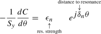
  Substituting $S_{y} = \sqrt {1 - |C|{ }^2}$ (Eq. 2.25) results in dC∕dθ differential equation under the form

  $$\displaystyle \begin{aligned} -\dfrac{1}{\sqrt{1 - |C|{}^2}} \dfrac{dC}{d\theta} = \epsilon_n \ e^{ \textstyle j \delta_n \theta} {} \end{aligned} $$

  (2.40)

Accelerating through a resonance, γ varies: γ ≡ γ(θ). This requires changing δ_nθ ≡ (Gγ − Gγ_n)θ to $\int _0^{\theta } (G\gamma - G\gamma _n) d\theta$. Introduce the crossing speed,

$$\displaystyle \begin{aligned} a = \dfrac{d}{d\theta} (G\gamma - G\gamma_n) =\Bigg[ \begin{array}{lll} G \dfrac{d\gamma}{d\theta} & ~ ~ & \text{imperfection resonance} \\ G \dfrac{d\gamma}{d\theta} \pm \dfrac{du_y}{d\theta} & & \text{intrinsic resonance} \end{array} {} \end{aligned} $$

(2.41)

Note that a possible variation of the betatron tune contributes to the crossing speed (“tune jump” technique to preserve polarization, see Chap. 5), consider constant vertical tune, here. Assume constant acceleration rate, this gives

$$\displaystyle \begin{aligned} G\gamma - G\gamma_n = a \theta \qquad \text{and} \qquad \int (G\gamma - G\gamma_n) d\theta = \dfrac{a\theta^2}{2}\end{aligned}$$

thus

$$\displaystyle \begin{aligned} -\dfrac{1}{\sqrt{1 - |C|{}^2}} \dfrac{dC}{d\theta} = \epsilon_n \ e^{ \textstyle j \dfrac{a \theta^2 }{2}} \quad (1) {}\end{aligned} $$

(2.42)

Now,

• introduce the angle φ between spin vector S and vertical axis, thus $\left [ \begin {array}{l} S_{y} = \cos \varphi \\ |C|=\sin \varphi \end {array} \right .$;

• and pose 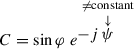; note also $\epsilon _n = |\epsilon _n| e^{ \textstyle j \, \mathrm {Arg} \, \epsilon _n}$, thus Eq. 2.42 takes the form

  $$\displaystyle \begin{aligned} -\dfrac{d}{d\theta} \left( \sin \varphi \ e^{ \textstyle -j \, \psi} \right) = |\epsilon_n| \ e^{ \textstyle j a \frac{\theta^2 }{2}} \ e^{ \textstyle j \mathrm{Arg} \, \epsilon_n} \ \cos \varphi\end{aligned}$$

  Finally, pose ϕ = ψ −Arg 𝜖_n, to get

  $$\displaystyle \begin{aligned} \dfrac{d}{d\theta} \left( \sin \varphi \ e^{ \textstyle -j \, \phi} \right) = - |\epsilon_n| \ e^{ \textstyle j a \frac{\theta^2 }{2}} \ \cos \varphi {} \end{aligned} $$

  (2.43)

  This is the differential equation which Froissart and Stora established, in 1959, in the context of plans for polarized ion beam acceleration in the Saturne synchrotron [10]. Given the present hypothesis of an isolated resonance, integration is over θ :   −∞ →  + ∞. Froissart and Stora solved it by a quantum mechanical approach where the equation to solve is linear, establishing that

  $$\displaystyle \begin{aligned} \cos \left[ \varphi(+\infty) - \varphi(-\infty)\right] = 2\, e^{ \textstyle -\dfrac{\pi}{2} \dfrac{|\epsilon_n|{}^2}{a}} -1 \end{aligned}$$

  a result commonly used under the form

  $$\displaystyle \begin{aligned} \dfrac{P_{\mathrm{final}}}{P_{\mathrm{initial}}} = 2\, e^{ \textstyle -\dfrac{\pi}{2} \dfrac{|\epsilon_n|{}^2}{a}} -1 {}\end{aligned} $$

  (2.44)

  with P_initial and P_final the beam polarization (average of spin states over particle ensemble) respectively far upstream and far downstream of an isolated resonance.

Figure 2.10 is a typical illustration of this depolarizing effect upon crossing of isolated resonances; each resonance in that series of four can be considered isolated as the distance to its neighbors is much greater than the width of the resonance (the width of a resonance is defined in Sect. 2.3.8).

Equation 2.44 shows that in the presence of a particular configuration of perturbing fields (which determines the resonance strength |𝜖_n|), the crossing speed a remains the main parameter. Three resonance crossing regimes can be distinguished:

• $\dfrac {|\epsilon _n|{ }^2}{a}$ large, $\Big [ \begin {array}{l} \text{strong resonance} \\ \text{slow crossing} \end {array}$ → P_f ≈−P_i, polarization flips;

• $\dfrac {|\epsilon _n|{ }^2}{a}$ small, $\Big [ \begin {array}{l} \text{weak resonance} \\ \text{fast crossing} \end {array}$ → P_f ≈ P_i, perturbative fields have marginal effect;

• intermediate regime → |P_f ∕ P_i| < 1 → polarization loss.

Preserving polarization requires one of the first two regimes, i.e., adiabatic crossing resulting in spin flip (at 99% for instance), or fast crossing resulting in marginal loss (1% for instance). Practical techniques to achieve that at discussed in Chap. 5.

Resonance Crossing Speed

• Case of constant tune $\left ( \dfrac {du _y}{dt}=0 \right )$:

  $a \equiv \dfrac {d(G \gamma - G\gamma _n)}{d\theta }= G \dfrac {d \gamma }{d\theta }$ is defined with respect to the azimuth variable θ. It is in that manner close to constant.

  $$\displaystyle \begin{aligned} \dfrac{d\gamma}{d\theta} = \dfrac{\Delta \gamma}{2\pi} = \dfrac{1}{2\pi} \dfrac{\Delta W}{E_0} \qquad \text{with} \ \Big[ \begin{array}{l} \Delta W\ \text{ the energy gain per turn}, \\ E_0 \ \text{ the rest energy of the particle} \end{array}\end{aligned}$$
  $$\displaystyle \begin{aligned} p = q \, B_{{y}_0}\rho_0 \quad \Rightarrow \dfrac{dp}{dt} = q \dot{B}_{{y}_0} \rho_0 = F \qquad \left( \dot{B} = \dfrac{dB}{dt} \right)\end{aligned}$$
  $$\displaystyle \begin{aligned} \text{work}\ \text{of }\ \text{F} \quad \Rightarrow \quad \Delta W = F\times 2\pi R = 2\pi R \, q \dot{B}_{{y}_0} \rho_0\end{aligned}$$

  thus

  $$\displaystyle \begin{aligned} \dfrac{d\gamma}{d\theta} = \dfrac{1}{2\pi} \dfrac{2\pi R \, q \dot{B}_{{y}_0} \rho_0}{E_0} = \dfrac{R \, \rho_0 \, \dot{B}}{E_0/q} \qquad \text{ and } \quad a = G \, \dfrac{d\gamma}{d\theta} = G\, \dfrac{R \, \rho_0}{E_0/q} \, \dot B\end{aligned}$$

• Case $\dfrac {du _y}{dt}eq 0$, “tune jump”:

  $$\displaystyle \begin{aligned} \dfrac{d(G \gamma- G\gamma_n)}{d\theta}= \dfrac{d\left(G \gamma - (\mathrm{n} \pm u_y)\right)}{d\theta}\end{aligned}$$

  and

  $$\displaystyle \begin{aligned} a= G \dfrac{d \gamma}{d\theta}\pm \dfrac{du_y}{d\theta}\end{aligned}$$

2.3.7 Spin Motion Through a Weak Resonance

In the case of a weak resonance, the spin differential equation of motion (Eq. 2.23, with Eq. 2.24) finds an analytical solution S_y(θ) [3]. This is an interesting case to explore at this allows an access to the details of spin motion, turn by turn through a resonance.

In the differential equation of motion through a resonance (Eq. 2.43) pose $\cos \varphi \approx 1$, i.e., angle to vertical axis left essentially unchanged by the crossing, this yields

$$\displaystyle \begin{aligned} \dfrac{d}{d\theta} \left( \sin \varphi \ e^{ \textstyle -j \, \phi} \right) = - |\epsilon_n| \ e^{ \textstyle j \frac{a \theta^2}{2}} {} \end{aligned} $$

(2.45)

Pose  $y = \sqrt { \dfrac {a}{\pi }} \theta$; in $d \left ( \sin \varphi \ e^{ \textstyle -j \, \phi } \right ) = - \sqrt { \dfrac {\pi }{a}} \ |\epsilon _n| \ e^{ \textstyle j \frac {\pi y^2}{2}} \ dy$, identify real and imaginary parts, this yields

$$\displaystyle \begin{aligned} \qquad \Bigg\{ \begin{array}{l} \sin \varphi \cos \phi = - \sqrt{ \frac{\pi}{a}} \ |\epsilon_n| \int_{-\infty}^y \cos \frac{\pi y^2}{2} \ dy \\[.5ex] \sin \varphi \sin \phi = + \sqrt{ \frac{\pi}{a}} \ |\epsilon_n| \int_{-\infty}^y \sin \frac{\pi y^2}{2} \ dy \end{array}\end{aligned}$$

and

(2.46)

A Check of the Weak Resonance Approximation Consider full crossing: y →∞. Integrate: $\int _{-\infty }^{\infty } \cos \frac {\pi y^2}{2} \ dy = 1$ and $\int _{-\infty }^{\infty } \sin \frac {\pi y^2}{2} \ dy = 1$, so that

$$\displaystyle \begin{aligned} \begin{array}{r} \sin^2 \varphi = \dfrac{2\pi}{a} \ |\epsilon_n|{}^2 \\ {} \text{thus} \ \sqrt{1- \sin^2 \varphi}= \cos \varphi \approx 1 -\dfrac{\pi}{a}|\epsilon_n|{}^2 \end{array} \Bigg\}\end{aligned}$$

a result in accord with the limited development of Froissart-Stora formula, namely (Eq. 2.44 with Δφ = φ − 0),

$$\displaystyle \begin{aligned} \cos \varphi = 2\, e^{ \textstyle -\dfrac{\pi}{2} \dfrac{|\epsilon_n|{}^2}{a}} -1 \approx 2 \, (1 -\dfrac{\pi}{2}\dfrac{|\epsilon_n|{}^2}{a} ) -1 = 1 -\dfrac{\pi}{a}|\epsilon_n|{}^2 \end{aligned}$$

Back to Eq. 2.46: introduce the Fresnel integrals

$$\displaystyle \begin{aligned} C(x) = \int_0^x \cos \dfrac{\pi t^2}{2} \ dt; \qquad S(x) = \int_0^x \sin \dfrac{\pi t^2}{2} \ dt\end{aligned}$$

and use

$$\displaystyle \begin{aligned} \int_{-\infty}^0 \cos \dfrac{\pi t^2}{2} \, dt = \int_0^{\infty} \cos \dfrac{\pi t^2}{2} \, dt = 0.5; \ \int_{-\infty}^0 \sin \dfrac{\pi t^2}{2} \, dt = \int_0^{\infty} \sin \dfrac{\pi t^2}{2} \, dt = 0.5\end{aligned}$$

This results in

$$\displaystyle \begin{aligned} \begin{array}{rcl} \begin{array}{ll} \text{For } y>0 \ \ i.e.,\ \theta >0 \quad \rightarrow & \overbrace{\sin^2 \varphi = \dfrac{\pi}{a} \ |\epsilon_n|{}^2 \left[ \left(0.5 + C(y)\right)^2 + \left( 0.5 + S(y)\right)^2 \right]}^{\text{downstream of the resonance}} \end{array} \\ \begin{array}{cc} \begin{array}{l} \text{For } y<0 \ \ {i.e.},\ \theta <0 \\ {} pose \ y=-x \ with \ x>0 \end{array} \rightarrow \underbrace{\sin^2 \varphi = \dfrac{\pi}{a} \ |\epsilon_n|{}^2 \left[ \left(0.5 - C(x)\right)^2 + \left( 0.5 - S(x)\right)^2 \right]}_{\text{upstream of the resonance}} \end{array} \\ {} \end{array} \end{aligned} $$

(2.47)

with the origin of the orbital angle θ at the resonance. A graph of the resulting $S_y=\cos \varphi =\sqrt {1-\sin ^2 \varphi }$ is displayed in Fig. 2.11.

Fig. 2.11

A graph of $S_y(\theta ) = \sqrt {1- \sin ^2 \varphi (\theta )}$ (solid curve; after Eq. 2.47). Numerical conditions are taken from AGS Booster, Gγ_n = ν_y resonance—see Sect. 14.1.1.9, markers are from turn-by-turn tracking simulations implemented there

2.3.8 Stationary Spin Precession; Width of a Resonance

If particle energy is fixed, so is the distance to the resonance

$$\displaystyle \begin{aligned} \delta_n = G\gamma - G\gamma_n = constant.\end{aligned}$$

Start from the spin motion equation s_π(θ) = C(θ) s_π,unpert.(θ) (Eq. 2.23) with $-\dfrac {1}{\sqrt {1 - |C|{ }^2}} \dfrac {dC}{d\theta } = \epsilon _n \ e^{ \textstyle j \delta _n \, \theta }$ (Eq. 2.40).

Look for a stationary solution for C(θ): $C(\theta ) = |{s_{\pi }}| \, e^{ \textstyle j \, \delta _n \, \theta }$. it comes

$$\displaystyle \begin{aligned} -\dfrac{1}{\sqrt{1 - |{s_{\pi}}|{}^2}} \left[ \dfrac{d|{s_{\pi}}|}{d\theta} + j\, \delta_n\, |{s_{\pi}}| \right] \, e^{ \textstyle j \, \delta_n\, \theta} = \epsilon_n \ e^{ \textstyle j \delta_n \, \theta}\end{aligned}$$

Look for a solution such that |s_π| = constant, thus $-\dfrac {j\, \delta _n\, |{s_{\pi }}|}{\sqrt {1 - |{s_{\pi }}|{ }^2}} = \epsilon _n$, so yielding

$$\displaystyle \begin{aligned} |{s_{\pi}}|{}^2 =\dfrac{1}{1 + \left( \dfrac{\delta_n}{|\epsilon_n|}\right)^2 } {} \end{aligned} $$

(2.48)

The physical quantity of interest is the polarization $\left < S_{y} \right > = \dfrac {n_+ - n_-}{n_+ + n_-}, n_{\pm }$: the number of particles with spin $\pm \dfrac {1}{2}$. From Eq. 2.48 it comes

$$\displaystyle \begin{aligned} \left< S_{y} \right> = \sqrt{1 - |{s_{\pi}}|{}^2 }= \dfrac{\delta_n}{\sqrt{\epsilon_n^2 +\delta_n^2}} {} \end{aligned} $$

(2.49)

and reciprocally

$$\displaystyle \begin{aligned} \dfrac{\delta_n}{|\epsilon_n|} = \dfrac{\left< S_{y} \right>}{\sqrt{1 - {\left< S_{y} \right>}^2}}\end{aligned}$$

|𝜖_n| is the resonance width (more rigorously, a measure of the latter, at 29.3% depolarization, Fig. 2.12).

Fig. 2.12

Polarization as a function of normalized distance δ_n∕|𝜖_n| to the resonance (Eq. 2.49). |𝜖_n| is the resonance width

The dependence of polarization upon distance to the resonance is displayed in Fig. 2.12. It is for instance 70.7%, 95% and 99% at distances respectively δ_n = |𝜖_n|, 3 |𝜖_n| and 7 |𝜖_n|.

2.3.9 Non-linear Resonances

Sextupoles excite non-linear depolarizing resonances [4]. These are driven by betatron motion, their effect on spin depends on both horizontal and vertical particle invariants, ε_x and ε_y (their effect on beam polarization depends on horizontal and vertical beam emittance): the greater ε_x,y, the greater the sextupole perturbative field

$$\displaystyle \begin{aligned} B_x = H\, x\, y = 2 H\, (B_0 \rho_0) \, x \, {y} {} \end{aligned} $$

(2.50)

Their location depends on both horizontal and vertical tunes:

$$\displaystyle \begin{aligned} G\gamma_n =n \pm u_x \pm u_y\end{aligned}$$

The perturbation function (Eq. 2.19) reduces to

$$\displaystyle \begin{aligned} f(\theta) = - S_{y} e^{ \textstyle -j \alpha} \lambda_x \dfrac{B_x}{B_0} = - 2 S_{y} e^{ \textstyle -j \alpha} \lambda_x H(\theta) \rho_0 \, x\, y \quad [ \text{with} \ \lambda_x = (1+G\gamma) \dfrac{R}{\rho_0}]\end{aligned}$$

so that (Eq. 2.26)

$$\displaystyle \begin{aligned} -\dfrac{1}{S_{y}} \dfrac{dC}{d\theta} = 2\lambda_x \rho_0 H(\theta) \, x(\theta) \, y(\theta) \, e^{ \textstyle jG \gamma \alpha} {} \end{aligned} $$

(2.51)

Substituting $x\, y (\theta ) = \left (F_x(\theta ) \, e^{ \textstyle j(u _{x} \theta + \varphi _{x})} + CC \right ) \left (F_y(\theta ) \, e^{ \textstyle j(u _{y} \theta + \varphi _{y})} + CC \right )$ wherein , yields

$$\displaystyle \begin{aligned} \begin{array}{rcl} & xy=\dfrac{1}{4}\sqrt{\textstyle \beta_x \dfrac{\varepsilon_x}{\pi}} \sqrt{\textstyle \beta_y \dfrac{\varepsilon_y}{\pi}} \left[ e^{\textstyle j \left( \int_0^s\frac{ds}{\beta_{x}} + \int_0^s\frac{ds}{\beta_{y}} - u_{x}\theta - u_{y}\theta \right) } e^{\textstyle j \left( u_{x}\theta + u_{y}\theta + \varphi_x + \varphi_y\right) } + CC \right. \\ & \left. + e^{\textstyle j \left( \int_0^s\frac{ds}{\beta_{x}} - \int_0^s\frac{ds}{\beta_{y}} - u_{x}\theta + u_{y}\theta \right) } e^{\textstyle j \left( u_{x}\theta - u_{y}\theta + \varphi_x - \varphi_y\right) } + CC \right] \end{array} \end{aligned} $$

(2.52)

Consider for instance the resonance Gγ_n = n − ν_x − ν_y, which stems from the term

$$\displaystyle \begin{aligned} \begin{array}{rcl} & - \dfrac{1}{S_{y}} \dfrac{dC}{d\theta} = \dfrac{1+G\gamma}{2} H(\theta)R \times \\ & \sqrt{\textstyle \beta_x \dfrac{\varepsilon_x}{\pi}} \, \sqrt{\textstyle \beta_y \dfrac{\varepsilon_y}{\pi}} \, e^{\textstyle j \left( \int_0^s\frac{ds}{\beta_{x}} + \int_0^s\frac{ds}{\beta_{y}} - u_{x}\theta - u_{y}\theta \right) } e^{\textstyle j \left( u_{x}\theta + u_{y}\theta + \varphi_x + \varphi_y\right) }\, e^{\textstyle j G\gamma \alpha } \end{array} \end{aligned} $$

(2.53)

In Eq. 2.51 re-write the factor e^jGγα  → e^{−jGγ(θ − α)} e^jGγθ, re-arrange, to get

$$\displaystyle \begin{aligned} \begin{array}{rcl} & - \dfrac{1}{S_{y}} \dfrac{dC}{d\theta} = \dfrac{1+G\gamma}{2} H(\theta)R \times \\ & \underbrace{ \sqrt{\textstyle \beta_x \dfrac{\varepsilon_x}{\pi}} \sqrt{\textstyle \beta_y \dfrac{\varepsilon_y}{\pi}} e^{\textstyle j \left( \int_0^s\frac{ds}{\beta_{x}} + \int_0^s\frac{ds}{\beta_{y}} - u_{x}\theta - u_{y}\theta -G\gamma (\theta - \alpha)\right) }}_{\text{1-turn periodic} } e^{\textstyle j \left( u_{x}\theta + u_{y}\theta + \varphi_x + \varphi_y\right) } {} \end{array} \end{aligned} $$

(2.54)

Expand the 1-turn periodic component in Eq. 2.55 in Fourier series, ∑_n𝜖_ne^−jnθ, the harmonic strength writes

$$\displaystyle \begin{aligned} \epsilon_n = \dfrac{1+G\gamma}{4\pi} R \oint H(\theta) \sqrt{\textstyle \beta_x \dfrac{\varepsilon_x}{\pi}} \sqrt{\textstyle \beta_y \dfrac{\varepsilon_y}{\pi}} e^{\textstyle j \left( \int_0^s\frac{ds}{\beta_{x}} + \int_0^s\frac{ds}{\beta_{y}} - u_{x}\theta - u_{y}\theta -G\gamma (\theta - \alpha)\right) } e^{\textstyle j n \theta } \, d\theta\end{aligned}$$

Near the resonance Gγ ≈ n − ν_x − ν_y, thus the previous expression reduces to

$$\displaystyle \begin{aligned} \epsilon_n = \frac{1+G\gamma}{4\pi} R \oint H(\theta) \sqrt{\textstyle \beta_x \dfrac{\varepsilon_x}{\pi}} \sqrt{\textstyle \beta_y \dfrac{\varepsilon_y}{\pi}} e^{\textstyle j \left( \int_0^s\frac{ds}{\beta_{x}} + \int_0^s\frac{ds}{\beta_{y}} + G\gamma \alpha \right) } \, d\theta\end{aligned}$$

In the thin-lens approximation, take ( Δθ)_Sextupole = L_i∕R the orbital extent of lens i located at s_i = s(θ = θ_i), the integral $\oint$ simplifies to a discrete sum over the lenses. Note (HL)_i the integrated sextupole strength, , α_i the cumulated orbit deviation at sextupole i, the resonance strength then writes

$$\displaystyle \begin{aligned} \epsilon_n = \dfrac{1 + G\gamma }{4\pi} \ \sum_{\mathrm{Sextu}} (HL)_i\, \sqrt{\beta_{x,i} \dfrac{\varepsilon_{x}}{\pi}} \sqrt{\beta_{y,i} \dfrac{\varepsilon_{y}}{\pi}} \, e^{\textstyle j \left( \int_0^{s_i} \frac{ds}{\beta_{x,i}} + \int_0^{s_i} \frac{ds}{\beta_{y,i}} +jG \gamma\alpha \right) } \end{aligned}$$

Distinguishing the real and imaginary components, the strength of the harmonics in the thin-lens approximation writes

$$\displaystyle \begin{aligned} \left\{ \begin{array}{r} \mathcal{R}e( \epsilon_n) \\ \mathcal{I} m(\epsilon_n) \end{array} \right\} = \dfrac{1+G\gamma}{4\pi}\, \sum_{\mathrm{Sextu}} \left\{ \begin{array}{l} \cos (G\gamma \alpha_i + \varphi_{x,i} + \varphi_{y,i})\\ \sin (G\gamma \alpha_i + \varphi_{x,i} + \varphi_{y,i})\end{array} \right\} (HL)_i \, \sqrt{\beta_{x,i} \dfrac{\varepsilon_{x}}{\pi}}\sqrt{\beta_{y,i} \dfrac{\varepsilon_{y}}{\pi}} {} \end{aligned} $$

(2.55)

with the betatron phase advance from the origin.

2.4 Homework

In Exercises 2.4 to 2.4, theoretical elements introduced in the course are used to build ad hoc elementary, short, numerical simulations aimed at producing the numerical results expected from theory. These exercises also allow additional, “hands-on”, insight in the arcanes of spin motion theory, spin motion in cyclic accelerators and the effects of such parameters as energy, perturbing fields, betatron motion frequency and amplitude. In order to complete and understand these simulations and their input data, it is necessary to have at hand the manual of the computer code used as this is where all useful explanations regarding optical components resorted to and their keywords, input and output data files and their content, etc., will be found. Note that any code with capabilities of spin tracking through arbitrary E and B fields, as necessitated in these three exercises, can be utilized; the code resorted to here and its manual can be downloaded from sourceforge [17] details regarding its utilization are given in due place in the exercises concerned, 2.4 to 2.4.

Exercises 2.4 to 2.4 are theoretical questions, only requiring paper and pencil.

Exercise 1: Low Energy Spin Rotator

This exercise serves two purposes: (1) moving a spin through a combined electric × magnetic field device and checking simulation outcomes against theoretical expectations, on the one hand, but also, (2) getting a taste of numerical simulation of spin motion through accelerator optical components.

Prior to injection into downstream stages, a linac for instance, spins generally need be set normal to the beam propagation axis, from their longitudinal orientation at the source. A Wien filter may be used for that: this is the case for instance in CEBAF electron injector (Fig. 8.4, p. 204) a similar device is under study for the EIC [18].

Working Hypotheses Refer to the reference frame in Fig. 2.13,

• the X axis is the electron propagation direction in the Wien filter,

  Fig. 2.13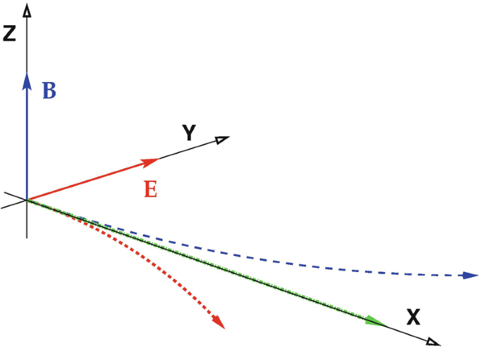

  

  Straight electron trajectory across a Wien filter spin rotator. Blue trajectory: case E = 0; Red trajectory: case B = 0

• take E ∥Y, B ∥Z, v ∥X,

• E_Y(X) and B_Z(X) fields are considered step functions in a first part of the simulations; yet field fall-offs do matter and are included in a second part.

• 1. Recall the relationship between E_Y and B_Z for a straight electron trajectory.

• 2. From the analogy between velocity and spin precession equations, namely (with ()′ = d()∕ds)

  $$\displaystyle \begin{aligned} \mathbf v{\, '} = \mathbf v \times \mathbf B/B\rho \quad \mathrm{and} \quad \mathbf S^{\,\prime} = \mathbf S \times \mathbf \Omega /B\rho \end{aligned}$$

  express the spin precession under the effect of this E, B crossed fields device, in terms of distance s, B_Z, E_Y, v∕c, particle rigidity Bρ and Wien filter length L.

• 3. Take electron energy 350 keV, L=1.5 m. Find the numerical values of E_Y and B_Z.

• 4. An input data file for the simulation of a 50 cm segment of the spin rotator is provided in [19]—README files are provided there as well, for guidance. In view of the next questions the input file is actually in two parts: WFSegment.dat which is specific to this question and WFSegment.inc which contains the 50 cm segment proper and called by the former, both available from [19].

  WFSegment.dat computes particle and spin motion through the 50 cm Wien filter segment, by stepwise numerical integration, and produces a graph of spin motion over the 50 cm; the simulation material includes the corresponding gnuplot script: gnuplot_spin.gnu, its content clarifies which computational output data, from which output file, are concerned in the present question.

  • 4.a It comes out of a preliminary run of WFSegment.dat (following the README file instructions) that the Wien filter E_Y and B_Z field values assigned in WFSegment.inc are not accurate: electron final transverse coordinates are not zero, its spin rotation is not 30^∘.

    Confirm this by running the simulation file as is and providing graphs of the electron trajectory and spin precession over the 50 cm segment. Find in the result listing the (present, incorrect) values of the trajectory coordinates and spin precession angle at the exit of this loosely tuned Wien filter.

  • 4.b In WFSegment.inc, update E_Y and B_Z to their theoretical values, as per question 3.

    Provide the new graphs of the electron trajectory, it should be straight along the X-axis, and of spin motion over the 150 cm Wien filter (as in Fig. 2.14), it should end up normal to the X-axis after a 150 cm path.

    Fig. 2.14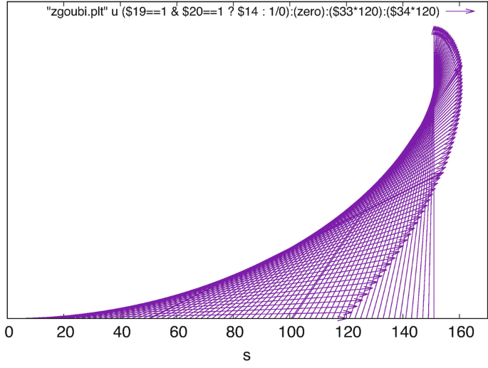

    

    Spin precession along the X axis, from longitudinal at s = 0 to ∥E at s = 1.5 m

  • 4.c Using the theoretical E_Y and B_Z values, compute the dependence of the final electron coordinates (position and angle) and spin precession angle, on the integration step size. Provide a graph. Explain what you observe.

    Hint: use the following form of REBELOTE do-loop command to repeat tracking through WIENFILT for a series of integration step size values:

    'REBELOTE' 100 0.1 0 1        ! Repeat the previous sequence, 100 times, and prior to each repeat, 1                                                      ! change value of one parameter, WIENFILT 80 0.01:10.           ! namely, number 80 (integration step size) in WIENFILT.

    Add FAISTORE[FNAME=zgoubi.fai] before REBELOTE, to store particle data at each pass.

    What is the maximum step size for a relative error on spin precession below 10⁻⁴?

• 5. Add λ_E ≈ λ_B ≈ 5 ∼ 7 cm long E and B field fall-off at both ends of the Wien filter 50 cm segment. Ensuring zero particle coordinates at exit and 30^∘ spin precession now requires adjusting the fields.

  A fitting procedure allows computing the matched values of E_Y and B_Z; their relative difference to the hard edge theoretical values is expected to be small.

  Provide graphs of the electron trajectory, and of E_Y(X) and B_Z(X).

• 6. The E and B fringe fields in a Wien filter actually have different extents. This causes an offset of particle trajectory.

  Keep the electric field entrance and exit fall-offs λ_E = 5 cm fixed, and vary the magnetic field fringe length in the range 3 ≤ λ_B ≤ 7 cm; re-match the field values to recover exit coordinates equal to zero together with 30^∘ spin precession angle.

  Reproduce Fig. 2.15: the series of trajectories, Y(X), obtained for this series of values of the ratio λ_E∕λ_B.

  Fig. 2.15

  

  A scan of the on-momentum orbit across the Wien filter, with varying fringe field extent ratio λ_E∕λ_B. The orbit is zero at entrance by hypothesis, and zeroed at the exit

  Provide a graph of the dependence on the ratio λ_E∕λ_B, of the relative variation of E_Y and B_Z.

  Hint: use the following form of REBELOTE do-loop command, placed after FIT, to repeat the fitting procedure for a series of λ_E∕λ_B values:

  'REBELOTE' 37 0.1 0 1   ! NPASS is of the form int∗(7[cm]-3[cm])+1 to allow for lambdaB/lambdaE=1. 2 WIENFILT 22 3.:7.                       ! vary lambda_B at entrance EFB from 3 to 7 cm. WIENFILT 52 3.:7.                           ! vary lambda_B at exit EFB from 3 to 7 cm.

Solution A detailed solution of this exercise is given in [20]. All computer code input files for questions 4–6 can be found in the USPAS Spin Class repository [20], where simulation result files (result listings, gnuplot scripts and graphs, etc.) can be found as well.

Exercise 2: Synchronized Torque

This exercise resorts to theory in order to build spin motion simulations; it includes the introduction of a local spin rotator and the investigation of subsequent resonant behavior (the spin rotator torque superposes to the uniform field, possibly synchronized with the betatron motion). It requires simulating orbital motion of a single proton in a uniform field (the field of a classical cyclotron, typically), on a constant radius orbit, thus at constant energy.

Simulation data files can be based on the following two, found in [20]: synchSpinTorque.INC.dat which computes the circular motion of a few protons in a uniform 5 kG field, and their spin motion, and the optical sequence file 60degSector.inc which is called by the former; both include comments, for guidance.

For each question, explain what is expected from theory, and compare with simulation outcomes. As a guidance, Fig. 2.16 gives an idea of expected outcomes.

• 1. Find the closed orbit for a 200 keV proton in that 5 kG uniform field.

  Fig. 2.16

  

  Left: vertical spin component as a function of orbital angle, for various Gγ values. Middle: spin motion on a sphere, some non-integer Gγ value. Right: spin motion on a sphere, integer Gγ; every turn the spin jumps by an angle equal to the spin rotator angle, 10^∘ here

• 2. Introduce a 30^∘ precession of the spin, rotation axis is the longitudinal axis (a local pure spin rotation may be applied as it avoids any perturbation of the orbital motion, a solenoid can be used otherwise).

  • 2.a Plot the vertical spin component as a function of orbital angle, over a few tens of turns.

  • 2.b Plot the projection of the spin vector motion in the horizontal plane.

  • 2.c Plot the projection of the spin vector motion on a sphere.

  • 2.d Compute the spin closed orbit vector at the origin of the optical sequence, and the spin tune.

• 3. Change the proton energy to 108.412 MeV, repeat questions 1 and 2.

  How many turns are needed to flip the spin?

• 4. Repeat for 370.082556 MeV.

Solution A detailed solution of this exercise is given in [19]. All computer code input files can be found in the USPAS Spin Class repository [20], where simulation result files (result listings, gnuplot scripts and graphs, etc.) can be found as well.

Exercise 3: Periodic Spin Precession in a Ring

This exercise is a follow up of the previous one, “Synchronized Torque”. Orbital motion of a single proton in a uniform field, on a constant radius orbit is considered again, here. The periodic solution of the spin equation of motion in a cyclic accelerator is investigated, it is known as the “stable spin precession direction”, or “spin closed orbit”.

Consider the motion of the spin of a particle on a closed orbit around the ring, in this configuration, a stable spin precession direction can be found, which closes on itself after a turn.

• 1. Find the closed spin precession solution at the location of the longitudinal kick (SPINR), in the different energy cases addressed in Exercise 2.2.

  Hint: A matching procedure can be used, with constraint equal initial and final spin coordinates.

• 2. Propagate that closed solution over a few turns around the ring. Produce a graph of s_π around the ring, in the laboratory frame. Repeat for the different energies (as in Fig. 2.17).

  Fig. 2.17

  

  Left: spin components as a function of orbital angle, Gγ = 2.5. Right: projection of spin motion in the bend plane, Gγ = 2

• 3. Prove that spins at an angle to the stable precession direction precess around the latter.

Solution A detailed solution of this exercise is given in [19]. All computer code input files can be found in the USPAS Spin Class repository [20], where simulation result files (result listings, gnuplot scripts and graphs, etc.) can be found as well.

Exercise 4: Strength of a Longitudinal Axis Spin Rotator

Show that if a device (known as a snake, see “Rotators and Snakes”, Chap. 4) is introduced which causes a spin rotation of angle ϕ_snake around the longitudinal axis, the strength of the integer resonance it induces is $|\epsilon _n^{\mathrm {snake}}| = \phi _{\mathrm {snake}} \, /2\pi$.

Solution The question is treated in Sect. 2.3.5.3.

Exercise 5: Orbit Distortion and Spin Rotator, Superposed

Consider a lattice featuring a vertical orbit distortion which excites imperfection resonances with strength 𝜖^imp. Assume that lattice includes a longitudinal spin rotator with resonance strength 𝜖^long..

Express the imperfection resonance strength resulting from the superposition of these two perturbative effects. Write the Froissart and Stora formula in that case.

(Hint: consider the derivation of Eq. 2.29).

Solution The following is a guidance, detailed calculation is left to the reader.

Consider the differential equation for C in the case of linear resonances (Eq. 2.26): two perturbative terms have to be retained, namely, B_x arising from a non-zero vertical closed orbit, and B_s arising from a longitudinal spin rotator. Thus, Eq. 2.27 features two series, one for 𝜖^imp, one for 𝜖^long., thus the complex strength is the sum of the two contributions,

$$\displaystyle \begin{aligned} \epsilon = \epsilon^{\mathrm{imp}} + \epsilon^{\mathrm{long.}}\end{aligned}$$

The Froissart and Stora formula (Eq. 2.44) in that case writes

$$\displaystyle \begin{aligned} \dfrac{P_{\mathrm{final}}}{P_{\mathrm{initial}}} = 2\, e^{ \textstyle -\dfrac{\pi}{2} \dfrac{|\epsilon^{\mathrm{imp}} + \epsilon^{\mathrm{long.}}|{}^2}{a}} -1\end{aligned}$$

Exercise 6: Strength of Coupling Resonances

Calculate the resonance strength series in the thin-lens approximation (i.e., in a similar form to Eq. 2.35) in the case of skew quadrupole fields.

Solution Skew quadrupoles, or quadrupole roll defects, cause horizontal field components of the form

$$\displaystyle \begin{aligned} B_x(\theta) = G\, x (\theta) = K_{sk}(\theta)\times B_0 \rho_0 \times {x}_{\beta}(\theta)\end{aligned}$$

with K_sk the field strength. These excite resonances at all Gγ_n = n ± ν_x.

Considering Eq. 2.31, getting the resonance strength is a matter of substituting K → K_sk and $y_{\beta }(\theta )= F_{y}(\theta ) \, e^{ \textstyle j(u _{y} \theta + \varphi _{y})} \ + CC \rightarrow x_{\beta }(\theta )= F_{x}(\theta ) \, e^{ \textstyle j(u _{x} \theta + \varphi _{x})} \ + CC$. Propagating these changes in Eq. 2.35 yields the coupling resonance strength

$$\displaystyle \begin{aligned} \left\{ \begin{array}{r} \mathcal{R}e( \epsilon_n^{\pm}) \\ \mathcal{I}\! m( \epsilon_n^{\pm}) \end{array} \right\} = \dfrac{1+G\gamma_n}{4\pi}\, \sum_{\mathrm{Qpoles}} \left\{ \begin{array}{l} \cos (G\gamma_n \alpha_i \pm \varphi_i)\\ \sin (G\gamma_n \alpha_i \pm \varphi_i)\end{array} \right\} (K_{sk}L)_i \, \sqrt{\beta_{x,i} \dfrac{\varepsilon_{x}}{\pi}}\end{aligned}$$

with $\varphi _i = \int _0^{s(\theta _i)} \dfrac {ds}{\beta _{x}}$ the horizontal betatron phase advance from the origin.

References

E. Grorud, J.L. Laclare, G. Leleux, Résonances de dépolarisation dans Saturne 2. Internal Rep. GOC-GERMA-75-48/TP-28, CEA Saclay (24 jullet 1975)
E. Grorud, J.L. Laclare, G. Leleux, Crossing of depolarization resonances in strongly modulated structures. IEEE Trans. Nucl. Sci. NS-26(3), 3209 (1979)
G. Leleux, Traversée des résonances de dépolarisation. Internal Report, Groupe Théorie, Laboratoire National Saturne, CEA Saclay (15 février 1991)
E. Grorud, J.L. Laclare, G. Leleux, Résonances de dépolarisation dans Saturne 2 (résonances systématiques d’ordre supérieur à 1). Rapport interne LNS-020, LNS CEN/Saclay (1975)
T. Aniel, J.L. Laclare, G. Leleux, A. Nakach, A. Ropert, Polarized particles at Saturne. J. Phys. Colloques 46(C2), C2-499-C2-507 (1985). https://hal.archives-ouvertes.fr/jpa-00224582/document
L.G. Ratner, T.K. Khoe, Acceleration of polarized protons in the zero gradient synchrotron (ZGS). IEEEE Trans. Nucl. Sci. NS-20(3), 217–220 (1973). https://doi.org/10.1109/TNS.1973.4327083. https://accelconf.web.cern.ch/p73/PDF/PAC1973_0217.PDF; Khoe, T., et al.: Acceleration of polarized protons to 8.5 GeV/c. Part. Accel. 6, 213 (1975) https://inspirehep.net/files/b19f7e869ddbb52e6f291bbc65b9d1f1
E.D. Courant, R.D. Ruth, The acceleration of polarized protons in circular accelerators. BNL 51270, Brookhaven National Laboratory (September 12, 1980)
L.H. Thomas, The kinematics of an electron with an axis. Lond. Edinb. Dublin Philos. Mag. J. Sci. 3(13), 1–22 (1927). https://doi.org/10.1080/14786440108564170
V. Bargmann, L. Michel, V.L. Telegdi, Precession of the polarization of particles moving in a homogeneous electromagnetic field. Phys. Rev. Lett. 2(10), 435 (1959)
M. Froissart, R. Stora, Dépolarisation d’un faisceau de protons polarisés dans un synchrotron. Nucl. Instrum. Methods 7, 297–305 (1959)
L.C. Teng, Deolarization of a polarized proton beam in a circular accelerator. Rep. FN-267 0100, Fermilab (November 1974)
B.W. Montague, Polarized beams in high energy storage rings. Phys. Rep. (Rev. Sect. Phys. Lett.) 113(1), 1–96 (1984)
J. Buon, J.P. Koutchouk, Polarization of electron and proton beams. Report CERN-SL-94-80-AP (1994). http://cds.cern.ch/record/269521/files/p879.pdf
S.R. Mane, Yu.M. Shatunov, K. Yokoya, Spin-polarized charged particle beams in high-energy accelerators. Rep. Prog. Phys. 68, 1997 (2005). http://iopscience.iop.org/0034-4885/68/9/R01
S.Y. Lee, Spin Dynamics and Snakes in Synchrotrons (World Scientific, 1997)
M. Conte, W. MacKay, An Introduction to the Physics of Particle Accelerators, 2nd edn. (World Scientific, 2008)
F. Méot, The ray-tracing code Zgoubi. NIM A 767, 112–125 (2014). Zgoubi Users’ Guide: https://sourceforge.net/p/zgoubi/code/HEAD/tree/trunk/guide/Zgoubi.pdf. Zgoubi download package at sourceforge: https://sourceforge.net/p/zgoubi/code/HEAD/tree/trunk/
F. Méot, E. Wang, Spin simulations in eRHIC Wien filter. Tech Note EIC/68; BNL-212123-2019-TECH (2019). https://technotes.bnl.gov/PDF?publicationId=212123
A link to the solutions of exercises 1-3 in USPAS web site: https://uspas.fnal.gov/materials/21onlineSBU/Spin-Dynamics/Home-work/Spin-Dynamics-and-Spinors/Solutions.shtml
A link to zgoubi input data files and result files for Exercises 1-3 in USPAS web site: https://uspas.fnal.gov/materials/21onlineSBU/Spin-Dynamics/Home-work/Spin-Dynamics-and-Spinors.shtml
Author information
Authors and Affiliations
Corresponding author
Editor information
Editors and Affiliations
Rights and permissions
Open Access This chapter is licensed under the terms of the Creative Commons Attribution 4.0 International License (http://creativecommons.org/licenses/by/4.0/), which permits use, sharing, adaptation, distribution and reproduction in any medium or format, as long as you give appropriate credit to the original author(s) and the source, provide a link to the Creative Commons license and indicate if changes were made.
The images or other third party material in this chapter are included in the chapter's Creative Commons license, unless indicated otherwise in a credit line to the material. If material is not included in the chapter's Creative Commons license and your intended use is not permitted by statutory regulation or exceeds the permitted use, you will need to obtain permission directly from the copyright holder.
Copyright information
© 2023 This is a U.S. government work and not under copyright protection in the U.S.; foreign copyright protection may apply
About this chapter
Cite this chapter
Méot, F. (2023). Spin Dynamics. In: Méot, F., Huang, H., Ptitsyn, V., Lin, F. (eds) Polarized Beam Dynamics and Instrumentation in Particle Accelerators. Particle Acceleration and Detection. Springer, Cham. https://doi.org/10.1007/978-3-031-16715-7_2
Download citation
DOI: https://doi.org/10.1007/978-3-031-16715-7_2
Published:
Publisher Name: Springer, Cham
Print ISBN: 978-3-031-16714-0
Online ISBN: 978-3-031-16715-7
eBook Packages: Physics and AstronomyPhysics and Astronomy (R0)