
Abstract
This chapter is a brief introduction to antennas and electromagnetic radiation, focusing on antennas for EMC tests. We skip the math intense part around Maxwell’s Equations.
The formulas and statements in this chapter apply to the far-field (not the near-field), free-space, matched impedances (of antennas and receiver/transmitter equipment), and matched polarization (of the electromagnetic waves and the antenna polarization).
Antennas do not match transmission line impedances to wave impedances. If they did, a 377 ℧ transmission line would radiate all its power without requiring an antenna. Describing an antenna as an impedance transformator is similar to telling a child that babies are delivered by storks. Both are explanations that may satisfy a certain audience, but neither is consistent with the actual physics.
— Dr. Todd Hubing
You have full access to this open access chapter, Download chapter PDF
Keywords
- Antennas
- Intended antennas
- Unintended antennas
- Radiated emission testing
- Radiated immunity testing
- Far-field antennas
- Near-field antennas
- Isotropic radiator
- Electric dipole
- Dipole antenna
- Monopole antenna
- Directivity
- Antenna gain
- Effective aperture
- Antenna factor
- Multipath effect
- Radiation from differential-mode current
- Radiation from common-mode current
- Free-space path loss
- Link budget
9.1 Antennas and EMC Testing
An antenna is an interface between radio waves propagating through space and electric currents moving along metal conductors. It can act as a receiver (converting electromagnetic waves from space into voltages and currents in a conductor) or as a transmitter (converting voltages and currents into electromagnetic waves).
In EMC compliance testing, antennas have two functions:
-
Radiated emission testing. Antennas act as receivers.
-
Radiated immunity testing. Antennas act as transmitters.
Moreover, a distinction is made between E-field and H-field antennas.
-
E-field antennas. Electric field antennas , for example: biconical antennas, bilogical antennas, horn antennas, log-periodic antennas, and electric near-field probes (see Fig. 9.1).
Fig. 9.1 
E-field antenna examples by Rohde & Schwarz. From left to right: double-ridged waveguide horn antenna R&S®HF907, log-periodic antenna R&S®HL223, biconical antenna R&S®HK116E, and ultralog antenna R&S®HL562E
-
H-field antennas. Magnetic field antennas are usually all kinds of loop antennas for the near- and the far-field (see Fig. 9.2).
Fig. 9.2 
H-field antenna examples by Rohde & Schwarz. From left to right: active loop antenna R&S®HFH2-Z2E, triple-loop antenna R&S®HM020E


And last but not least, antennas are divided into near-field and far-field antennas:
-
Near-field antennas. Dedicated near-field antennas are called near-field probes (see Fig. 9.3). Electric and magnetic near-field probes are often used during EMC troubleshooting to identify unintentional radiators on PCBAs or unintended radiation through slots of enclosures. Magnetic field immunity tests are usually performed in the near-field of a loop antenna (e.g. at f = 50 Hz or 60 Hz).
Fig. 9.3 
EMC near-field probes R&S®HZ-15 with oscilloscope R&S®RTO2000 by Rohde & Schwarz. H-field near-field probes have loops, E-field probes not
-
Far-field antennas. Far-field antennas are used for EMC compliance emission and immunity tests (see Fig. 9.1). In some cases, far-field antennas are also used for near-field radiated immunity tests (radiated fields in close proximity [6]).

9.2 Isotropic Radiator
A spherical isotropic radiator (isotropic antenna) radiates equally in all directions (from one single point) and therefore has no directivity. Such an antenna does only exist in theory.
Let us define S [W/m2] as the power density of the field around an antenna at a given distance d [m]. The average power density S [W/m2] of an isotropic radiator is simply the radiated power P rad [W] by the antenna divided by the surface area of the spherical surface [m2] at a distance d [m] from the center of the radiator [11]:
where,
-
P rad = radiated power by an isotropic radiator in [m2]
-
d = distance from the isotropic radiator to the spherical surface in [m]
9.3 Antenna Directivity D
The directivity D of an antenna is defined as the ratio of the radiation intensity in a given direction from the antenna to the radiation intensity averaged over all directions. Thus, the directivity is an antenna parameter that measures the degree to which the emitted radiation is concentrated in a single direction. Figure 9.4 shows the radiation pattern (power density) of a transmitting antenna with directivity compared to an isotropic radiator. Directivity is also defined for receiving antennas. The directivity when receiving is equal to the directivity when transmitting.

Signal strength of a spherical isotropic radiator vs. an antenna with directivity (gain)
9.4 Antenna Gain G
Every real-world antenna has a directivity—meaning: it does not radiate equally in every direction. This leads us to the term antenna gain . The antenna gain G is a key performance number that combines the antenna’s directivity D and electrical efficiency e 0 [2]:
where,
-
e 0 = radiation efficiency of antenna (dimensionless)
-
D = directivity of antenna (without any losses, dimensionless)
For a loss-free antenna: G = D. The antenna gain G is defined as the ratio of the power radiated in the desired direction of an antenna compared to the power radiated from a reference antenna (e.g., isotropic radiator or dipole) with the identical power input (this means the antenna’s electrical efficiency factor P rad∕P t, which considers the antenna losses, is already taken into account in gain G) [11]. The antenna gain with reference to an isotropic radiator G i or to a λ∕2-dipole antenna G d is defined as:
where,
-
G i = gain of an antenna with reference to an isotropic radiator (dimensionless)
-
G d = gain of an antenna with reference to a λ∕2-dipole antenna (dimensionless)
Antenna gains are often given in [dBi] and [dBd]:
The antenna gains of loss-free λ∕2-dipoles and λ∕4-monopoles compared to an isotropic radiator are [2]:
Now, we are ready to calculate the often used terms: effective isotropic radiated power (EIRP ) and effective radiated power (ERP ) [9]:
where,
-
EIRP = RMS input power required to lossless isotropic radiator to give the identical maximum power density far from the antenna as the actual antenna in [W]
-
ERP = RMS input power required to lossless λ∕2-dipole to give the identical maximum power density far from the antenna as the actual antenna in [W]
-
P t = power input to the transmitting antenna in [W]
-
G i = antenna gain compared to isotropic radiator (dimensionless)
-
G d = antenna gain compared to λ∕2-dipole (dimensionless)
Assuming line of sight and free space (Fig. 9.5), the maximum power density S max [W∕m2] at a distance d [m] from the transmitting antenna (in the direction of the transmitting antenna’s main-lobe and in the far-field) can be written as:
where,
-
EIRP = RMS input power required to lossless isotropic radiator to give the identical maximum power density far from the antenna as the actual antenna in [W]
Fig. 9.5 
Transmitting and receiving antennas in free-space
-
d = distance from the transmitting antenna (in the far-field) in [m]

The term realized antenna gain G realized does not only include the antenna efficiency (ohmic losses, etc.) but also the impedance mismatch loss and is given as [1]:
where,
-
G i = antenna gain, compared to a spherical isotropic radiator (dimensionless)
-
\(| \underline {\varGamma }| =\) magnitude of the complex reflection coefficient between the signal generator or amplifier and the antenna (dimensionless)
9.5 Effective Aperture Ae
The effective area of an antenna is also called effective aperture A e [m2]. The effective aperture represents the ratio of power P r [W] (output power of the receiving antenna) to the power density S r [W∕m2] of the electromagnetic wave at the receiving antenna [2]:
where,
-
P r = RMS output power at the receiving antenna terminals in [W]
-
S r = power density S r at the receiving antenna in [W∕m2]
The maximum effective aperture A em [m2] for any antenna is [2]:
where,
-
λ = wavelength of the sinusoidal incident wave—which must be matched with the receiving antenna’s polarization—in [m]
-
G i = antenna gain of the receiving antenna (dimensionless)
The antenna gain G i can be expressed as a function of the maximum effective aperture A em [m2] and the wavelength λ [m] of the incident wave:
9.6 Antenna Factor AF
The antenna factor AF is a function of the signal’s frequency f [Hz] and is used to calculate the received field strength E [V/m] or H [A/m] based on the measured voltage V r [V] at the receiving antenna’s terminals [11]:
where,
-
E = RMS value of the electric field strength at the receiving antenna in [V/m]
-
H = RMS value of the magnetic field strength at the receiving antenna in [S/m]
-
V r = RMS value of the voltage at the receiving antenna’s terminals in [V]
In case of matched impedances at the receiving antenna’s terminals (Fig. 9.6), free space, a plane wave, and aligned receiving antenna to the polarization of the incident wave, we can write:
In case of free space and a plane wave, we can set λ = c∕f and η = η 0 = 120π ℧ in Eq. 9.21 and get:
where,
-
P r = RMS output power at the receiving antennas terminals in [W]
Fig. 9.6 
Simplified equivalent circuit of a receiving antenna with open load circuit voltage \( \underline {V}_0\) [V], antenna impedance \( \underline {Z}_a\) [Ω], receiver impedance \( \underline {Z}_r\) [Ω], and voltage at the receiving antenna terminals \( \underline {V}_r\) [V]
-
S r = power density S r at the receiving antenna in [W∕m2]
-
A em = maximum effective aperture of the receiving antenna (which requires alignment of the wave and the receiving antenna polarization) in [m2]
-
V r = RMS voltage at the receiving antenna terminals in [V]
-
\(\operatorname {Re}( \underline {Z}_r) =\) real value of the impedance of the receiver at the receiving antenna’s terminals in [Ω]
-
η = intrinsic impedance (in the far-field: Z w is equally to the intrinsic impedance η) of the incident plane wave at the receiving antenna in [Ω]
-
E = RMS value of the electric field strength at the receiving antenna in [V/m]
-
λ = wavelength of the sinusoidal incident plane wave in [m]
-
G ir = antenna gain of the receiving antenna (dimensionless)

Incase of Z r = 50 ℧, we can write:
where,
-
AFE = antenna factor of an E-field antenna in case of a plane wave (far-field) in free-space, a 50 ℧-system and matched polarization of the incident E-field and the antenna in [1/m]
-
λ = wavelength of the sinusoidal incident plane wave in [m]
-
G ir = antenna gain of the receiving antenna (dimensionless)
The antenna factor AF is often given in decibel:
9.7 Ground Plane Reflection and Multipath Effect
Assuming a transmitting and a receiving antenna placed above a reflective ground plane, where the receiving antenna and the ground plane are in the far-field of the transmitting antenna (see Fig. 9.7). The received field at the receiver antenna is the sum of the direct wave \(\overrightarrow {E}_d\) [V/m] and the reflected wave \(\overrightarrow {E}_r\) [V/m]:

Ground plane and receiving antenna are in the far-field of the transmitter
where,
-
\(\overrightarrow {E}_{sum} =\) E-field sum of direct and reflected waves at receiving antenna in [V/m]
-
\(\overrightarrow {E}_d =\) E-field at the receiving antenna from direct path in [V/m]
-
\(\overrightarrow {E}_r =\) E-field at the receiving antenna from reflected path in [V/m]
This phenomena is called multipath effect . The field strength |E sum| [V/m] at the receiving antenna depends on the distances the waves have traveled, the polarization of the antennas, the reflection coefficient \( \underline {\varGamma }\) of the ground plane, the attenuation α [1/m] of the media, and the frequency f [Hz] of the signal. Assuming that the ground plane and the receiving antenna are in the far-field of the transmitting antenna (so that R rad is not influenced by the ground plane), a perfectly conducting ground plane (\( \underline {\varGamma } = +1\) or − 1 [2]) and a lossless media (α = 0), the reflective field strength |E r| [V/m] could be as high as the field strength of the direct wave |E d| [V/m]. However, it could also happen that both fields cancel each other out at the receiving antenna. This means:
9.8 Intended Antennas
In EMC, the term intended antenna denotes an antenna for generating or receiving a specific electric, magnetic, or electromagnetic field in a predefined setup.
9.8.1 E-Field Antennas and Emission Testing
Radiated emission EMC standards like CISPR 11 [8], CISPR 32 [3], or FCC Part 15 [4] specify the radiated emission limits in [μV/m] or [dBμV/m]. Therefore, E-field antennas are used as receiving antennas (Fig. 9.8). In other words, the physical quantity of interest is the E-field [dBμV/m], and the measured physical quantity is the voltage V measure [dBμV] at the measurement equipment (e.g., spectrum analyzer or EMI receiver). The field strength of the E-field at the antenna can be calculated like this:
where,
-
E = RMS field strength of the E-field at the antenna in [dBμV/m]
Fig. 9.8 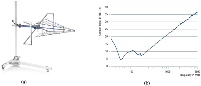
Example of an EMC emission and immunity testing E-field antenna. (a) Wideband biconilog antenna R&S®HL562E and frequency range from 30 MHz to 6 GHz. (b) Antenna factor of the wideband biconilog antenna R&S®HL562E by Rohde & Schwarz
-
AFE = antenna factor of an E-field antenna in [dB(1/m)]
-
Losses = losses of all cables and connectors from the receiver antenna to the measurement equipment (e.g., spectrum analyzer) in [dB]
-
V measure = measured RMS voltage at the measurement equipment (e.g., spectrum analyzer) in [dBμV]

9.8.2 E-Field Antennas and Immunity Testing
The physical quantity of interest for many radiated immunity EMC standards (like IEC 61000-4-3 [5]) is the E-field at a certain distance d (e.g., E = 10 V/m at d = 10 m). Therefore, E-field antennas like bilogical, log-periodic, or horn antennas are used—basically the identical antennas as for E-field emission testing.
From the antenna fundamentals from above, we know how to calculate the maximum power density S max [W/m2] at a distance d [m] for a transmitting antenna in free space with antenna gain G it and power P t [W] at the transmitting antenna terminals:
where,
-
S max = maximum power density for the input power of P t to the antenna at distance d (in case of matched polarization, main lobe, free space, and line of sight in the far-field) in [W/m2]
-
EIRP = RMS input power required to lossless isotropic radiator to give the identical maximum power density far from the antenna as the actual antenna in [W]
-
d = distance from the transmitting antenna (in the far-field and in the direction of the antenna’s main lobe) in [m]
-
P t = RMS power input to the transmitting antenna in [W]
-
G it = antenna gain of the transmitting antenna compared to an isotropic radiator (dimensionless)
Furthermore, we know the power density S [W/m2] of a plane wave in free space (far-field: wave impedance Z w [Ω] is equal characteristic impedance η 0 = 120π ℧) is given as [11]:
where,
-
E = RMS value of the electric field strength in [V/m]
-
η 0 = 120π ℧ = intrinsic impedance of free-space in [Ω]
If we combine Eqs. 9.31 and 9.32, we can determine the field strength E [V/m] at a given distance d [m] from the antenna for a given transmitting antenna input power P t [W]:
where,
-
E = RMS field strength of the electric field at distance d from the transmitting antenna for input power P t (assuming free space, line of sight, distance d in the far-field and in the direction of the transmitting antenna’s main lobe and matched polarization to the transmitting antenna) in [V/m]
-
P t = RMS power input to the transmitting antenna in [W]
-
G it = antenna gain of the transmitting antenna compared to an isotropic radiator (dimensionless)
-
G it[dBi] = antenna gain of the transmitting antenna compared to an isotropic radiator in [dBi]
-
d = distance from the transmitting antenna in [m]
Thus, the required input power P t [W] of a transmitting antenna for achieving a desired field strength E [V/m] at a given distance d [m] is (in free space, no reflective ground plane):
where,
-
P t = RMS input power at the transmitting antenna’s input terminals for achieving electric field strength E at distance d (assuming free space, line of sight, distance d in the far-field and in the direction of the transmitting antenna’s main lobe and matched polarization to the transmitting antenna) in [W]
-
E = RMS field strength of the electric field in [V/m]
-
G it = antenna gain of the transmitting antenna compared to an isotropic radiator (dimensionless)
-
G it[dBi] = antenna gain of the transmitting antenna compared to an isotropic radiator in [dBi]
-
d = distance from the transmitting antenna in [m]
9.8.3 H-Field Antennas and Emission Testing
Magnetic radiated emission EMC standards like MIL-STD-461 (RE101, f = 30 Hz to 100 kHz) require H-field loop antennas as receiving antennas (Fig. 9.9). In case the antenna factor is given in [dB(S/m)], the field strength of the H-field at the antenna can be calculated like this:
where,
-
H = RMS field strength of the H-field at the antenna in [dBμA/m]
Fig. 9.9 
Example of an emission testing H-field antenna. (a) A.H. Systems Inc. SA-560 passive loop antenna. (b) Coil factor of the passive loop antenna SAS-560 by A.H. Systems. The passive loop antenna SAS-560 was specifically designed for tests according to MIL-STD-461 RE101
-
AFH = antenna factor of an H-field antenna in [dB(S/m)]
-
Losses = losses of all cables and connectors from the receiver antenna to the measurement equipment (e.g., spectrum analyzer) in [dB]
-
V measure = measured RMS voltage at the measurement equipment (e.g., spectrum analyzer) in [dBμV]

In case the antenna factor for the receiving loop antenna is given in [dBpT/μV], the field strength of the H-field at the antenna can be calculated like this:
where,
-
H = RMS field strength of the H-field at the antenna in [dBpT]
-
AFH = antenna factor of an H-field antenna in [dBpT/μV]
-
Losses = losses of all cables and connectors from the receiver antenna to the measurement equipment (e.g., spectrum analyzer) in [dB]
-
V measure = measured RMS voltage at the measurement equipment (e.g., spectrum analyzer) in [μV]
9.8.4 H-Field Antennas and Immunity Testing
Radiated magnetic field EMC immunity standards, like IEC 61000-4-8 [7] (f = 50 Hz and 60 Hz) or MIL-STD-461 (RS101, f = 30 Hz to 100 kHz) require induction coils as transmitting antennas. In contrast to the E-field EMC tests—where the identical antennas are used for immunity and emission tests—the H-field immunity tests specify dedicated antennas, which are different from the H-field emission measurements.
Two important properties of an induction coil for H-field immunity tests are:
-
Homogeneity. Magnetic field immunity tests often require that the field strength should not vary more than, e.g., ±3 dB (see Fig. 9.10) over the volume of the EUT. The magnetic field homogeneity over a given volume is dependent on the induction coil. Details about the induction coils and the test setups are given in the respective EMC standards.
Fig. 9.10 
H-field homogeneity of a 1×1 m square loop antenna [7]. (a) 3 dB—area in the plane to the loop antenna. (b) 3 dB—area orthogonal to the loop antenna
-
Induction coil factor. The induction coil factor is the antenna factor of an induction coil. It describes the ratio between the magnetic field strength H [A/m] generated by an induction coil of given dimensions and the corresponding current I [A] value. The field is measured at the center of the coil plane without the EUT.

The manufacturer of an induction coil for magnetic immunity tests specifies in the datasheet of the coil antenna:
-
The test volume and position of the homogeneous magnetic field region
-
The operation frequency (range) of the antenna
-
The coil factor
The magnetic field strength H [A/m] at the position of interest (relative to the induction coil) can be calculated like this:
where,
-
H = RMS value of the magnetic field in the area of interest in [A/m]
-
c f = coil factor of the induction coil for a given frequency (range) f and a predefined volume (at a defined relative position to the induction coil) in [(A/m)/A]
-
I = RMS value of the current flowing through the induction coil in [A]
9.9 Unintended Antennas
Current loops, PCB structures, cables, or slots may act as unintended antennas . As a result, they receive or emit electromagnetic radiation unintentionally.
9.9.1 E-Field from Differential-Mode Currents in Small Loops
Let us assume a setup like shown in Fig. 9.11 where the following is given [11]:
-
Electrically small current loop (circumference < λ∕4), so that the current distribution (magnitude, phase) is constant along the current loop.
Fig. 9.11 
Radiated emissions E DM [V/m] due to differential-mode current I DM [A] around a current loop with area A [m2]. The direction of the electric field E DM [V/m] is parallel to the wires
-
Measurement point of the E-field is in the far-field.

Given the points above, the maximum electric field E DM,max [V/m] caused by a differential-mode current \( \underline {I}_{DM}\) [A] can be approximated as [11]:
where,
-
E DM,max = maximum RMS field strength radiated by electrically small current loop with area A and differential current I DM in [V/m]
-
I DM = RMS value of the differential-mode current in [A]
-
f = frequency of the sinusoidal current signal in [Hz]
-
A = area of the current loop in [m2]
-
d = distance to the center of the current loop in [m]
Reducing unintended radiation emissions due to a small differential-mode current loop gives the following options:
-
1.
Reducing the current amplitude. It is usually not practical to reduce the amplitude of the signal current \( \underline {I}_{DM}\) [A] because the amplitude was initially set due to functional reasons.
-
2.
Reducing the frequency or the amplitude of high-frequency harmonics. Let us assume the signal is a digital signal. Because the radiated emissions are proportional to the square of the frequency f 2 [Hz], amplitudes of the higher-frequency harmonics of a digital signal should be kept low by increasing the rise /fall time of the digital signal. Section 5.3 describes how to reduce the amplitude of the high-frequency harmonics of a digital signal.
-
3.
Reducing the current loop area. Loop areas can often not be changed without an extensive redesign. Therefore, loop areas should be considered early in the design phase.
Differential-mode currents do not radiate efficiently, and in practice, radiated emissions due to differential-mode currents are seldom an issue. Usually, the common-mode currents along cables are the root cause for high radiated emissions.
9.9.2 E-Field from Common-Mode Currents in Short Cables
Let us assume a setup like shown in Fig. 9.12 where the following is given [11]:
-
Electrically short cable length l [m] (e.g., l < λ∕4 [10]), so that the current distribution (magnitude, phase) is constant along the conductor.
Fig. 9.12 
Radiated emissions E CM [V/m] due to common-mode current I CM [A] through two closely spaced parallel conductors of length l < λ∕4. The direction of the electric field E CM [V/m] is parallel to the wires
-
Measurement point of the E-field is in the far-field.

Given the points above, the maximum electric field E CM,max [V/m] caused by the common-mode current \( \underline {I}_{CM}\) [A] can be approximated as [11]:
where,
-
E CM,max = maximum RMS field-strength radiated by electrically short cable of length l and common-mode current I CM in [V/m]
-
I CM = RMS value of the common-mode current in [A]
-
f = frequency of the sinusoidal current signal in [Hz]
-
l = length of the conductor or transmission line in [m]
-
d = distance to the center of the cable in [m]
Because common-mode currents are normally not required for system operation, the first rule is to avoid them. Once the common-mode currents are here: reduce them. One of the most common options to reduce common-mode currents is adding a clamp ferrite over the cable or wires, which are causing unintended radiated emissions. More information about cable mount ferrite beads can be found in Sect. 11.5.1 on page 169.
9.9.3 Maximum E-Field from Common-Mode Signals
Section 9.9.2 does only consider short cables (antennas) compared to the wavelength λ [m]. Therefore, these cables are not very effective radiators, which does not mean that they will never lead to failed EMC emission tests. Nonetheless, things get even worse when cable lengths l [m] match a multiple of a quarter wavelength nλ∕4 [m]. This section presents simple approximations for the worst-case emissions from given common-mode voltages and currents.
9.9.3.1 Generic Calculation of Maximum E-Field
Let us assume a sinusoidal signal with a RMS voltage V RMS [V] that drives a resonant structure like a λ∕4-monopole antenna. As a result, the current distribution along the antenna has a RMS value of I RMS [A]. Assuming a lossless antenna (R loss = 0 ℧), where the antenna input impedance \( \underline {Z}_{in}\) [Ω] is:
we can calculate the radiated power P rad [W] of this lossless antenna as [11]:
Combining Eqs. 9.34 and 9.41 for a lossless transmitter (where directivity D is equal the antenna gain G i), we get:
This leads us to the maximum radiated field-strength E max [V/m] at the resonance of a lossless antenna with matched impedance, matched polarization, and line-of-sight path:
where,
-
E max = maximum E-field at distance d for matched impedances, matched polarization, line-of-sight path, and a lossless antenna driven by V RMS in [V/m]
-
V RMS = RMS voltage that drives the lossless antenna in [V]
-
I RMS = RMS value of the current distribution along the lossless antenna in [A]
-
R rad = radiation resistance of the lossless antenna (function of frequency) in [Ω]
-
η 0 = 120π ℧ = intrinsic impedance of free space in [Ω]
-
G i = D = antenna gain of the lossless antenna (dimensionless)
-
d = distance from the antenna, where E max is measured in [m]
9.9.3.2 Maximum E-Field for a Given Common-Mode Current
Assuming a common-mode current \( \underline {I}_{CM}\) [A] flows along a resonant structure (e.g., a cable). When in resonance (and only then!), the maximum electric field-strength E max [V/m] can be approximated based on Eq. 9.43 as:
where,
-
E max = maximum RMS E-field at distance d for matched impedances, matched polarization, line-of-sight path, and a resonant structure driven by I CM in [V/m]
-
I CM = RMS common-mode current that flows along the resonant structure in [A]
-
R rad = radiation resistance in [Ω] (λ∕2-dipole: 73 ℧, λ∕4-monopole: 36.5 ℧)
-
η 0 = 120π ℧ = intrinsic impedance of free-space in [Ω]
-
G i = antenna gain (λ∕2-dipole, 1.64; λ∕4-monopole, 3.28)
-
d = distance from the antenna, where E max is measured in [m]
9.9.3.3 Maximum E-Field for a Given Common-Mode Voltage
Assuming a common-mode voltage \( \underline {V}_{CM}\) [V] that drives a resonant structure (e.g., a cable). When in resonance (and only then!), the maximum electric field-strength E max [V/m] can be approximated based on Eq. 9.43 as:
where,
-
E max = maximum RMS E-field at distance d for matched impedances, matched polarization, line-of-sight path, and a resonant structure driven by V CM in [V/m]
-
V CM = RMS common-mode voltage that drives the resonant structure in [V]
-
R rad = radiation resistance in [Ω] (λ∕2-dipole, 73 ℧; λ∕4-monopole, 36.5 ℧)
-
η 0 = 120π ℧ = intrinsic impedance of free space in [Ω]
-
G i = antenna gain (λ∕2-dipole, 1.64; λ∕4-monopole, 3.28)
-
d = distance from the antenna, where E max is measured in [m]
9.9.4 Maximum E-Field from PCB with Attached Cable
Let us assume a setup like shown in Fig. 9.13 where the following is given:
-
A cable connected to a PCBA, which is driven by an unintended antenna-mode (common-mode) voltage \( \underline {V}_{AM}\) [V] and connected to an infinite ground plane at the other end.
Fig. 9.13 
Unintended antenna structure: cable connected to a PCBA on one end and attached to an infinite ground plane at the other end. An antenna-mode (common-mode) voltage \( \underline {V}_{AM}\) [V] drives an antenna-mode current \( \underline {I}_{AM}\) [A] through a cable
-
The structure in Fig. 9.13 is essentially an unbalanced monopole antenna, which reaches the maximum radiation E AM,max [V/m] when the cable length l cable [m] and/or the board size l board [m] are a quarter wavelength λ∕4 [m] or larger.
-
Measurement point of the E-field is in the far-field, over a reflective ground plane.

The maximum RMS value of the electric field E AM,max [V/m] measured in a anechoic chamber (with a reflecting ground plane) caused by an antenna-mode signal with \( \underline {V}_{AM}\) [V] and \( \underline {I}_{AM}\) [A] that drives the board-cable structure as an antenna can be approximated like this [12,13,14]:
where,
and
-
V AM = antenna-mode RMS voltage driving the monopole antenna (cable) in [V]
-
I AM,max = highest antenna-mode RMS current that exists on the cable in [A]
-
R min = 36.5 ℧ = radiation resistance of a resonant λ∕4-monopole antenna in [Ω]
-
l board = effective board length in [m]
-
l cable = cable length in [m]
-
L = length of the PCBA (board) in [m]
-
W = width of the PCBA (board) in [m]
-
k board = impact of board size l board on R min in case l board ≤ λ∕4
-
k cable = impact of cable length l cable on R min in case l cable ≤ λ∕4
-
d = distance to the radiating structure (PCBA, cable) in [m]
-
f = frequency of the sinusoidal signal \( \underline {V}_{AM}\) in [Hz]
-
λ = wavelength of the sinusoidal signal \( \underline {V}_{AM}\) in [m]
-
c = 2.998 ⋅ 108 m/sec = speed of light
9.10 Free-Space Path Loss
The term free-space loss, free-space path loss factor, or free-space path loss (FSPL) refers to the attenuation of the electromagnetic field between a transmitting and a receiving antenna in case the space between the antennas is free of obstacles and a line-of-sight path through free-space.
A way to calculate the FSPL is given by the Friis transmission equation , which assumes matched impedances, matched polarization of the transmit, and receive antennas and that the receiving antenna is in the far-field [11]:
where,
-
P r = output power at the receiving antennas terminals in [W]
-
P t = input power to the transmitting antenna in [W]
-
G ir = antenna gain of the transmitting antenna (dimensionless)
-
G ir = antenna gain of the receiving antenna (dimensionless)
-
λ = wavelength of the sinusoidal electromagnetic wave in [m]
-
d = distance between the transmitting and receiving antennas in [m]
-
f = frequency of the sinusoidal electromagnetic wave in [Hz]
-
\(c = 1/(\sqrt {\mu _0\epsilon _0}) = 2.998 \cdot 10^{8}\) m/sec = speed of light
9.11 Link Budget
The link budget is an accounting of all of the power gains and losses that a signal experiences along a transmission path (from transmitter to receiver). If you want to calculate the received power P r [dBm] for a given transmitter-receiver setup (transmitter, frequency, antennas, distance, etc.), you calculate the link budget. In simple terms, this means:
If we rewrite the link budget formula above in a little more detailed way, we get:
where,
-
P r = maximum received power, e.g., at a spectrum analyzer (connected via coaxial cable with the receiving antenna) in case of the receiving antenna in the far-field, in the direction of the main lobe of the transmitting antenna, matched impedances, matched polarization of the incident wave, and the receiving antenna and free space in [dBm]
-
P t = output power of, e.g., a signal generator (connected via coaxial cable with the transmitting antenna) in [dBm]
-
G ir = antenna gain of the transmitting antenna in [dBi]
-
G ir = antenna gain of the receiving antenna in [dBi]
-
L t = transmitter losses (coaxial cable, connectors, etc.) in [dB]
-
FPSL = free-space path loss in [dB]
-
L misc = miscellaneous losses (fading, polarization mismatch, etc.) in [dB]
-
L r = receiver losses (coaxial cable, connectors, etc.) in [dB]
9.12 Summary
-
Antennas Types and EMC There are dedicated antennas for the near-field and the far-fields and for the E- and H-fields (Table 9.1).
Table 9.1 Antenna types and EMC -
Antenna directivity D. The directivity D of an antenna is defined as the ratio of the radiation intensity in a given direction from the antenna to the radiation intensity averaged over all directions. The directivity does not take losses of the antenna into account.
-
Antenna gain G. The antenna gain G corresponds to the directivity D of the antenna, but with losses (efficiency) of the antenna taken into account.
-
Antenna factor (AF). Antennas for EMC tests are typically characterized by their antenna factors AF.
-
Unintended antennas. Common-mode currents are more likely to lead to undesired radiation than differential-mode currents (compare Eqs. 9.38 vs. 9.39). From an EMC point of view, common-mode currents through unintended antennas should be prevented by design (radiated emissions are proportional to the common-mode current).
-
Free-space path loss (FSPL). The FSPL is a practical and simplified approximation for the attenuation of an electromagnetic wave in the far-field (in the case of line of sight and free space).
References
ANTENNAS & ACCESSORIES, CATALOG 2020/2021. Rohde & Schwarz GmbH & Co. KG. Mar. 2020.
Constantine A. Balanis. Antenna Theory - Analysis and Design. 3rd edition. John Wiley & Sons Inc., 2005.
CISPR 32 Electromagnetic compatibility of multimedia equipment – Emission requirements. International Electrotechnical Commission (IEC). 2015.
Code of Federal Regulations - Title 47 - Chapter I - Subchapter A - Part 15 (FCC 47 CFR Part 15). Federal Communication Commission (FCC, USA). 2021.
Electromagnetic compatibility (EMC) - Part 4–3 : Testing and measurement techniques - Radiated, radio-frequency, electromagnetic field immunity test. International Electrotechnical Commission (IEC). 2020.
Electromagnetic compatibility (EMC) - Part 4–39: Testing and measurement techniques - Radiated fields in close proximity - Immunity test. International Electrotechnical Commission (IEC). 2017.
Electromagnetic compatibility (EMC) - Part 4–8: Testing and measurement techniques - Power frequency magnetic field immunity test. International Electrotechnical Commission (IEC). 2009.
Industrial, scientific and medical equipment - Radio-frequency disturbance characteristics - Limits and methods of measurement. International Electrotechnical Commission (IEC). 2015.
Wendy M. Middleton. Reference Data For Engineers: Radio, Electronics, Computer and Communications. 9th edition. John Wiley & Sons, Inc., 2001.
Henry W. Ott. Electromagnetic Compatibility Engineering. John Wiley & Sons Inc., Sept. 11, 2009.
Clayton R. Paul. Introduction to electromagnetic compatibility. 2nd edition. John Wiley & Sons Inc., 2008.
Todd Hubing Shaowei Deng and Daryl Beetner. “Estimating Maximum Radiated Emissions From Printed Circuit Boards With an Attached Cable”. In: IEEE TRANSACTIONS ON ELECTROMAGNETIC COMPATIBILITY Vol. 50.No. 1 (2008), pp. 215–218.
Changyi Su. “DEVELOPMENT OF REDUCED COMPLEXITY MODELS FOR ELECTROMAGNETIC MODELING”. PhD thesis. Clemson University, 2011. URL: https://tigerprints.clemson.edu/cgi/viewcontent.cgi?article=1788&context=all_dissertations.
Changyi Su and Dr. Todd H Hubing. Calculating Radiated Emissions due to I/O Line Coupling on Printed Circuit Boards using the Imbalance Difference Method. Tech. rep. Clemson University, 2011.
Author information
Authors and Affiliations
Rights and permissions
Open Access This chapter is licensed under the terms of the Creative Commons Attribution 4.0 International License (http://creativecommons.org/licenses/by/4.0/), which permits use, sharing, adaptation, distribution and reproduction in any medium or format, as long as you give appropriate credit to the original author(s) and the source, provide a link to the Creative Commons license and indicate if changes were made.
The images or other third party material in this chapter are included in the chapter's Creative Commons license, unless indicated otherwise in a credit line to the material. If material is not included in the chapter's Creative Commons license and your intended use is not permitted by statutory regulation or exceeds the permitted use, you will need to obtain permission directly from the copyright holder.
Copyright information
© 2023 The Author(s)
About this chapter

Cite this chapter
Keller, R.B. (2023). Antennas. In: Design for Electromagnetic Compatibility--In a Nutshell. Springer, Cham. https://doi.org/10.1007/978-3-031-14186-7_9
Download citation
DOI: https://doi.org/10.1007/978-3-031-14186-7_9
Published:
Publisher Name: Springer, Cham
Print ISBN: 978-3-031-14185-0
Online ISBN: 978-3-031-14186-7
eBook Packages: EngineeringEngineering (R0)