Elements of Graphs and Complexity Theory

Abstract

This chapter recalls some elements and definitions in graph theory and complexity theory. On the one hand, basic algorithmic courses very often include graph algorithms. Some of these algorithms have simply been transposed to solve difficult optimization problems in a heuristic way. On the other hand, it is important to be able to determine whether a problem falls into the category of difficult problems. Indeed, one will not develop a heuristic algorithm if there is an efficient algorithm to find an exact solution. Another objective of this chapter is to make the book self-contained.

Before designing a heuristic method to find good solutions to a problem, it is necessary to be able to formalize it mathematically and to check that it belongs to a difficult class. Thus, this chapter recalls some elements and definitions in graph theory and complexity theory in order to make the book self-contained. On the one hand, basic algorithmic courses very often include graph algorithms. Some of these algorithms have simply been transposed to solve difficult optimization problems in a heuristic way. On the other hand, it is important to be able to determine whether a problem falls into the category of difficult problems. Indeed, one will not develop a heuristic algorithm if there is an efficient algorithm to find an exact solution.

1 Combinatorial Optimization

The typical field of application of metaheuristics is combinatorial optimization. Let us briefly introduce this domain with an example of a combinatorial problem: the coloring of a geography map. It is desired to assign a color for each country drawn on a map so that any two countries that have a common border do not receive the same color. In Fig. 1.1, five different colors are used, without worrying about the political attribution of the islands or enclaves.

Fig. 1.1

An old European map colored with five colors (taking the background into account)

This is a combinatorial problem. Indeed, if there are n areas to color with five colors, there are 5ⁿ different ways to color the map. Most of these colorings are unfeasible because they do not respect the constraint that two areas with a common border do not receive an identical color. The question could be asked whether there is a feasible coloring using only four colors. More generally, one may want to find a coloring using a minimum number of colors. Consequently, we are dealing here with a combinatorial optimization problem.

How to model this problem more formally? Let us take a smaller example (see Fig. 1.2): can we color Switzerland (s) and neighboring countries (Germany d, France f, Italy, Liechtenstein, and Austria a) with three colors?

Fig. 1.2

Switzerland and its neighbor countries that we want to color. Each country is symbolized by a disk, and a common border is symbolized by a line connecting the corresponding countries. The map coloring can be transformed into the coloring of the vertices of a graph

A first model can be written using 18 binary variables that are put into equations or inequations. Let us introduce variables x _s1, x _s2, x _s3, x _d1, x _d2, …, x _a3 that should either take value 1 or 0. x _ik = 1 means that country i receives color k. Now, we can impose that a given country i receives exactly one color by writing the equation: x _i1 + x _i2 + x _i3 = 1. To avoid assigning the same color to two countries (i and j) having a common border, we can write three inequalities (one for each color):

$x_{i1} + x_{j1} \leqslant 1$, $x_{i2} + x_{j2} \leqslant 1$ and $x_{i3} + x_{j3} \leqslant 1$.

Another model can introduce 18 Boolean variables b _s1, b _s2, b _s3, b _d1, b _d2, …, b _a3 that indicate the color (1, 2 or 3) of each country. b _ik = true means that country i receives color k. Now, we write a long Boolean formula that is true if and only if there is a feasible 3-coloring. First of all, we can impose that Switzerland is colored with at least one color: b _s1 ∨ b _s2 ∨ b _s3. But it should not receive both color 1 and color 2 at the same time: This can be written $\overline {b_{s1}\land b_{s2}}$, which is equivalent to $\overline {b_{s1}}\lor \overline { b_{s2}}$. Then, it should also not receive both color 1 and color 3 or color 2 and color 3. Thus, to impose that Switzerland is colored with exactly 1 color, we have the conjunction of four clauses:

$$\displaystyle \begin{aligned} (b_{s1}\lor b_{s2}\lor b_{s3})\land(\overline{b_{s1}}\lor\overline{ b_{s2}})\land(\overline{b_{s1}}\lor\overline{ b_{s3}})\land(\overline{b_{s2}}\lor\overline{ b_{s3}})\end{aligned}$$

For each of the countries concerned, it is also necessary to write a conjunction of four clauses but with the variables corresponding to the other countries. Finally, for each border, it is necessary to impose that the colors on both sides are different. For example, for the border between Switzerland and France, we must have:

$$\displaystyle \begin{aligned} (\overline{b_{s1}}\lor\overline{ b_{f1}}) \land (\overline{b_{s2}}\lor\overline{ b_{f2}}) \land (\overline{b_{s3}}\lor\overline{ b_{f3}})\end{aligned}$$

Now a question arises: how many variables are needed to color a map with n countries which have a total of m common borders using k colors? Another one is: how many constraints (equation, inequation, or clauses ) are needed to describe the problem? First, it is necessary to introduce n ⋅ k variables. Then, for each country, we can write one equation or $1+\frac {k\cdot (k - 1)}{2}$ clauses to be sure that each country receives exactly one color. Finally, for each border, it is necessary to write one inequation or m ⋅ k clauses. The problem of coloring such a map with k colors has a solution if and only if there is a value 1 or 0 for each of the binary variables or a value true or false for each of the Boolean variables such that all the constraints are simultaneously satisfied.

The Boolean model is called the satisfiability problem (SAT) . It plays a central role in complexity theory. This extensive development is to formalize the problem by a set of equations or inequations or by a unique, long Boolean formula, but does not inform us yet how to discover a solution!

An extremely primitive algorithm to find a solution is to examine all the possible values for the variables (there are 2^nk different sets of values), and for each set, we have to check if the formula is true.

As modeled above, coloring a map is a decision problem. Its solution is either true (a feasible coloring with k colors exists) or false (this is impossible). Assuming that an algorithm $\mathscr {A}$ is available to obtain the values to assign to the variables so that all equations or inequations are satisfied or the Boolean formula is true—or to say that such values do not exist—is it possible to solve the optimization problem: which is the minimum number k of colors for having a feasible coloring?

One way to answer this question is to note that we need at most n colors for n areas and to assign a distinct color to each of them. As a result, we know that an n-coloring exists. We can apply the algorithm $\mathscr {A}$ to ask for an n − 1 coloring, then n − 2, etc. until getting the answer that no coloring exists. The ultimate value for which the algorithm has found a solution corresponds to an optimal coloring.

A faster technique is to proceed by a dichotomy: rather than reducing the number of color by one unit at each call of algorithm $\mathscr {A}$, two values, k _min and k _max, are stored so that it is known that there is no feasible coloring (respectively, a feasible coloring exists). By eliminating the case of the trivial map that has no boundary, we know that we can start with k _min = 1 and k _max = n. The algorithm is asked for a $k = \lfloor \frac {k_{min} + k_{max}}{2}\rfloor$ coloring. If the answer is yes, we modify $k_{max} \gets \lfloor \frac {k_{min} + k_{max}}{2}\rfloor$; if the answer is no, we change $k_{min} \gets \lfloor \frac {k_{min} + k_{max}}{2}\rfloor$. The method is repeated until k _max = k _min + 1. This value corresponds to the optimum number of colors. So, an optimization problem can be solved with an algorithm answering the corresponding decision problem.

1.1 Linear Programming

Linear programming is an extremely useful tool for mathematically modeling many optimization problems. Mathematical programming is the selection of a best element, with regard to some quantitative criterion, from some set of feasible alternatives. When the expression of this criterion is a linear function and all feasible alternatives can be described by means of linear functions, we are talking about linear programming.

A linear program under canonical form can be mathematically written as follows:

$$\displaystyle \begin{aligned} \mbox{Maximize} && z & = & c_1 x_1 & + & c_2 x_2 & + & \cdots & + & c_n x_n \end{aligned} $$

(1.1)

$$\displaystyle \begin{aligned}\mbox{Subject} && & & a_{1 1} x_1 & + & a_{1 2} x_2 & + & \cdots & + &a_{1 n} x_n & \leqslant b_1 & \end{aligned} $$

(1.2)

$$\displaystyle \begin{aligned} \mbox{to:} && & & a_{2 1} x_1 & + & a_{2 2} x_2 & + & \cdots & + & a_{2 n} x_n & \leqslant b_2 &\\ && && \cdots & & & & \cdots & & \cdots & & & \\ && & & a_{m 1} x_1 & + & a_{m 2} x_2 & + & \cdots & + &a_{m n} x_n & \leqslant b_m &\\ {} && & & & & & & & & x_j & \geqslant 0\ (j = 1, \dots, n) \\ \end{aligned} $$

(1.3)

[-28pt]

z represents the objective function and x _j the decision variables. For a production problem, the c _j can be seen as revenues, the b _i being quantities of raw material available and the a _ij the unit consumption of material i for the production of good j.

The canonical form of linear programming is not limiting, in the sense that any linear program can be expressed under this form. Indeed, if the objective is to minimize z, this is equivalent to maximizing − z; if a variable x can be either positive or negative or null, it can be substituted by x″ − x′, where x″ and x′ must be nonnegative; finally, if we have an equality constraint a _i1 x ₁ + a _i2 x ₂ + ⋯ + a _in x _n = b _i, it can be replaced by the constraints $a_{i1} x_1 + a_{i2} x_2 + \dots + a_{in} x_n \leqslant b_i$ and $-a_{i1} x_1 - a_{i2} x_2 - \dots - a_{in} x_n \leqslant -b_i$.

The map coloring problem can be modeled by a slightly special linear program. For that, one introduces the variables y _k that indicate if the color k is used (y _k = 1) or not (y _k = 0, k = 1, …, n) in addition to the variables x _ik that indicate if the area i receives the color k. The integer linear program allows formalizing the optimization version of the map coloring problem:

$$\displaystyle \begin{aligned} \begin{array}{rcl} {} \mbox{Minimize} & z &\displaystyle = \sum_{k = 1}^n{y_k} \end{array} \end{aligned} $$

(1.4)

$$\displaystyle \begin{aligned} \begin{array}{rcl} \mbox{Subject to:} & &\displaystyle \\ {} \sum_{k = 1}^n{x_{ik}} & = &\displaystyle 1\quad i = 1, \dots, n \end{array} \end{aligned} $$

(1.5)

$$\displaystyle \begin{aligned} \begin{array}{rcl} {} x_{ik} - y_k & \leqslant&\displaystyle 0\quad i, k = 1, \dots, n \end{array} \end{aligned} $$

(1.6)

$$\displaystyle \begin{aligned} \begin{array}{rcl} {} x_{ik} + x_{jk} & \leqslant &\displaystyle 1\quad \forall(i, j)\ \mbox{having a common border}, \end{array} \end{aligned} $$

(1.7)

$$\displaystyle \begin{aligned} \begin{array}{rcl} & &\displaystyle \ \ \quad k = 1, \dots, n\\ {} x_{ik}, y_k \ & \in &\displaystyle \{0, 1\} \end{array} \end{aligned} $$

(1.8)

The objective (1.4) is to use the minimum number of colors. The first set of constraints (1.5) imposes that each vertex receives exactly one color; the second set (1.6) ensures that a vertex is not assigned to an unused color; the set (1.7) prevents the same color to be assigned to contiguous areas. The integrity constraints (1.8) can also be written with linear inequalities ($y_k \geqslant 0,\quad y_k \leqslant 1,\quad y_k \in \mathbb {Z}$).

Linear programming is a very powerful tool for modeling and formalizing problems. If there are no integrity constraints, problems with thousands of variables and thousands of constraints can be effectively solved. In this case, the resolution is barely more complex than the resolution of a system of linear equations. The key limitation is essentially due to the memory space required for data storage as well as any numerical problems that may occur if the data is poorly conditioned.

However, integer linear programs, like the coloring problem expressed above, are generally difficult to solve, and specific techniques should be designed. Metaheuristics are among these techniques.

If the formulation of a problem under the form of a linear program allows a rigorous modeling, it does not help our mind much for its solving. Indeed, the sight is the most important of our senses. The adage says a small drawing is better than a long speech. The graphs represent a more appropriate way for our spirit to perceive a problem. Before presenting other models for the coloring problem (see Sect. 2.8), some definitions in graph theory are recalled so that this book is self-contained.

1.2 A Small Glossary on Graphs and Networks

Graphs are a very useful tool for problem modeling when there are elements that have relationships between them. The elements are represented by a point and two related elements are connected by a segment. Thus, the previously seen map coloring problem can be drawn by a small graph, as shown in the Fig. 1.2.

1.2.1 Undirected Graph, Vertex, (Undirected) Edge

An undirected graph G is a pair of a set V  of elements called vertices or nodes and of a set E of undirected edges , each of them associated with a (unordered) pair of nodes, which are their endpoints. Such a graph is noted as G = (V, E). A vertex of a graph is represented by a point or a circle. An edge is represented by a line.

If two vertices v and w are joined by an edge, they are adjacent . The edge is incident with v and w.

When several edges connect the same pair of vertices, we have multiple edges . When both endpoints of an edge are the same vertex, this is a loop .

When $V = \varnothing$ (and $E = \varnothing$), we have the null graph. When $V \neq \varnothing$ and $E = \varnothing$, we have an empty graph. A graph with no loop and no multiple edges is a simple graph ; otherwise, this is a multigraph . Figure 1.2 depicts a simple graph.

The complement graph $\overline {G}$ of a simple graph G has the same set of vertices and two distinct vertices of $\overline {G}$ are adjacent if and only if they are not adjacent in G.

1.2.2 Directed Graph, Arcs

In some cases, the relationships between the pairs of elements are ordered. This is a directed graph or digraph . The edges of a digraph are called the arcs or directed edges . An arc is represented by an arrow connecting its endpoints.

It is therefore necessary to distinguish both endpoints of an arc (i, j). The starting point i is called the tail and the arrival point j is the head. j is a direct successor of i and i is a direct predecessor of j. The set of direct successors of a node i is written Succ(i), and the set of its direct predecessors Pred(i).

An arc whose tail and head are the same vertex is also called a loop, as for the undirected case. Two arcs having the same tail and the same head are parallel or multiple arcs.

1.2.3 Incidence Matrix

The incidence matrix A of a graph with n vertices and m arcs and without loops is a matrix with m columns and n rows. The coefficients a _ij(i = 1, …, n, j = 1, …, m) of A are defined as follows:

$$\displaystyle \begin{aligned} a_{ij} = \left\{ \begin{array}{rl} -1 & \text{if } i \text{ is the tail of the arc } (i,j)\\ 1 & \text{if } j \text{ is the head of the arc } (i,j)\\ 0 & \text{else} \end{array} \right. \end{aligned}$$

In the case of an undirected graph, both endpoints are represented by 1s in the vertex-edge incidence matrix. It should be noticed that the incidence matrix does not allow to properly represent loops.

1.2.4 Adjacency Matrix

The adjacency matrix of a simple undirected graph is a square matrix with the coefficient a _ij is 1 if vertices i and j are adjacent and 0 otherwise.

1.2.5 Degree

The degree of a vertex v of an undirected graph, noted deg(v), is the number of edges that are incident to v. A loop increases by 2 the degree of a vertex. A vertex of degree 1 is pendent. A graph is regular if all its vertices have the same degree. For a directed graph, the outdegree of a vertex, noted deg ⁺(v), is the number of arcs having v as tail. The indegree of a vertex, deg ⁻(v), is the number of arcs having v as head.

1.2.6 Path, Simple Path, Elementary Path, and Cycle

A path (also referred to as a walk ) is an alternating sequence of vertices and edges, beginning and ending with a vertex, such that each edge is surrounded by its endpoints. A simple path (also referred to as a trail ) is a walk for which all edges are distinct. An elementary path (also simply referred to as a path) is a trail in which all vertices (and therefore also all edges) are distinct. A cycle is a trail where the first vertex is corresponding to the last vertex. A simple cycle is a cycle in which the only repeated vertex is the first/last one. The length of a walk is its number of edges. Contrary to French, there is no difference in the wording between undirected and directed graphs. So, the edges, paths, etc. must be qualified with “directed” or “undirected.” However, arcs are always directed edges.

1.2.7 Connected Graph

An undirected graph is connected if there is a path between every pair of its vertices. A connected component of a graph is a maximal subset of its vertices (and incident edges) such that there is a path between every pair of the vertices. A directed graph is strongly connected if there is a directed path in both directions between any pair of vertices.

1.2.8 Tree, Subgraph, and Line Graph

A tree is a connected graph without cycles (acyclic). A leaf is a pendent vertex of a tree. A forest is a graph without cycles. Each of its connected component is a tree. A rooted tree is a directed graph with a unique path from one vertex (the root of the tree) to each remaining vertex.

G′ = (V ′, E′) is a subgraph of G = (V, E), if V ′⊂ V  and E′ has all the edges of E with both endpoints in V ′. A spanning tree of a graph G is a subgraph of G which is a tree.

The line graph L(G) of a graph G is built as follows (see also Fig. 2.12):

• Each edge of G is associated with a vertex of L(G).

• Two vertices of L(G) are joined by an edge if their corresponding edges in G share an endpoint.

1.2.9 Eulerian, Hamiltonian Graph

A graph is Eulerian if it contains a walk that uses every edge exactly once. A graph is Hamiltonian if it contains a walk that uses every vertex exactly once. Sometimes, Eulerian and Hamiltonian graphs are limited to the case when there is a cycle that uses every edge or every vertex exactly once (the first/last vertex excepted).

1.2.10 Complete, Bipartite Graphs, Clique, and Stable Set

In a complete graph , every two vertices are adjacent. All edges that could exist are present. A bipartite graph G = (V, E) is such that V = V ₁ ∪ V ₂, $V_1 \cap V_2 = \varnothing$ and each edge of E has one endpoint in V ₁ and the other in V ₂. A clique is a maximal set of mutually adjacent vertices that induces a complete subgraph. A stable set or independent set is a subset of vertices that induces a subgraph without any edges. A number of elements defined in the above paragraphs are illustrated in Fig. 1.3

Fig. 1.3

Basic definition of graph components

1.2.11 Graph Coloring and Matching

The vertex coloring problem has been used as an introductory example in the Sect. 1.1 devoted to combinatorial optimization. A proper coloring is a labeling of the vertices of a graph by elements from a given set of colors such that distinct colors are assigned to the endpoints of each edge. The chromatic index of a graph G, noted χ(G), represents the minimum number of colors of a proper coloring of G. An edge coloring is a labeling of the edges by elements from a set of colors. The proper edge coloring problem is to minimize the number of colors required so that two incident edges do not receive the same color. A matching is a set of edges sharing no common endpoints. A perfect matching is a matching that matches every vertex of the graph.

1.2.12 Network

In many situations, a weight w(e) is associated with every edge e of a graph. Typically, w(e) is a distance, a capacity or a cost. A network, noted R = (V, E, w), is a graph together with a function $w: E \rightarrow \mathbb {R}$. The length of a path in a network is the sum of the weights of its edges.

1.2.13 Flow

A classical problem in a directed network R = (V, E, w) is to assign a nonnegative flow x _ij to each edge e = (i, j) so that ∑_{j ∈ Succ(i)} x _ij =∑_{k ∈ Pred(i)} x _ki ∀i ∈ V, i ≠ s, t. Vertex s is the source-node and t the sink-node. If $0 \leqslant x_{ij} \leqslant w_{ij} \forall (i, j) \in E$, the flow from s to t is feasible.

A cut is a partition of the vertices of a network R = (V, E, w) into two subsets A ⊂ V  and $\overline {A} \subset V$. The capacity of a cut from A to $\overline {A}$ is the sum of the weight of the edges that have one endpoint in A and the other in $\overline {A}$.

Network flows are convenient to model problems that have, at first glance, nothing in common with flows, like resource allocation problems (see, e.g., Sect. 2.5.1). Further, in this chapter, we will review some well-known and effective algorithms for the minimum spanning tree, the shortest path, or the optimum flow in a network. Other problems, like graph coloring, are intractable. The only algorithms known to solve them require a time that can grow exponentially with the size of the graph.

Complexity theory focuses on classifying computational problems into easy and intractable ones. Metaheuristics have been designed to identify satisfactory solutions to difficult problems, while requiring a limited computing effort. Before developing a new algorithm on the basis of the principles of metaheuristics, it is essential to be sure the problem addressed is an intractable one and that there are not already effective algorithms to solve it. The rest of this chapter exposes some theoretical bases in the field of classification of problems according to their difficulty.

2 Elements of Complexity Theory

The purpose of complexity theory is to classify the problems in order to predict whether they will be easy to solve. To limit ourselves to sequential algorithms, we consider, very roughly, that an easy problem can be solved by an algorithm, which computational effort is limited by a function that polynomially depends on the size of the data to be treated. We can immediately dare why the difficulty limit must be on the class of polynomials and not on that of logarithmic, trigonometric, or exponential functions.

The reason is very simple: we can perfectly conceive that more effort is required to process a larger volume of data, eliminating nongrowing functions like trigonometric ones. Limited to sequential methods, it is clear that each record must be read at least once, which implies a growth in the number of operations at least linear. This eliminates logarithmic, square root, etc. functions. Naturally, for a parallel treatment of the data by several tasks, it is quite reasonable to define a class of problems (very easy), requesting a number of operations and memory per processor increasing at most logarithmically with the data volume. An example of such a problem is finding the largest number of a set.

Finally, we must consider that an exponential function (in the mathematical sense, such as 2^x, but also extensions such as $x^{\log x}$, x! or x ^x) always grow faster than any polynomial. This growth is incredibly impressive.

Let us examine the example of an algorithm that requires 3⁵⁰ operations for a problem with 50 elements. If this algorithm is run on a machine able to perform 10⁹ operations per second, the machine will not complete its work before 23 million years. By comparison, solving a problem with ten elements—five times smaller—with the same algorithm would take only 60 microseconds.

Hence, it would not be reasonable in practice to consider as easy a problem requiring an exponential number of operations to be solved. But combinatorial problems include an exponential number of solutions. As a result, complete enumeration algorithms, sometimes called “brute force,” cannot be reasonably considered acceptable. Thus, the computation of a shortest path between two vertices of a network cannot be solved by enumerating the complete set of all paths since it is exponentially large. Algorithms using mathematical properties of the shortest walks must be used. These algorithms perform a number of steps that is polynomial in the network size. On the one hand, finding a shortest walk is an easy problem. On the other hand, finding a longest (or a shortest) path (without circuits or without visiting twice the same vertex) between two vertices is an intractable problem , because no polynomial algorithm is known to solve it.

Finally, we must mention that the class of polynomials has an interesting property: it is closed. The composition of two polynomials is also a polynomial. In the context of programming, it means that a polynomial number of calls to a subroutine that requires a computational effort that grows polynomially with the data size leads to a polynomial algorithm.

2.1 Algorithmic Complexity

Complexity theory and algorithmic complexity should not be mixed up. As already mentioned, complexity theory focuses on the problem classification. The purpose of algorithmic complexity is to evaluate the resources required to run a given algorithm. It is therefore possible to develop an algorithm of high complexity for a problem belonging to the class of “simple” problems.

To be able to put a problem into a complexity class, we will not assume the use of any given algorithm to solve this problem, but we will analyze the performance of the best possible algorithm—not necessarily known—for this problem and running on a given type of machine. We must not confuse the simplicity of an algorithm (expressed, e.g., by the number of lines of code needed to implement it) and its complexity. Indeed, a naive algorithm can be of high algorithmic complexity.

For instance, to test if an integer p is prime, we can try to divide it by all the integers between 2 and $\sqrt {p}$. If all these divisions have a reminder, we can conclude that p is prime. Otherwise, there is a certificate (a divider of p) proving that p is not prime. This algorithm is easy to implement. However, it is not polynomial in the size of the data. Indeed, just n =log₂(p) bits are required to code the number p. Therefore, the algorithm requires a number of divisions proportional to 2^n∕2, which is not polynomial.

However, it has been proven in 2002 that there is a polynomial algorithm to detect if a number p is prime. As we can expect, this algorithm is undoubtedly a sophisticated one. Its analysis and implementation is just a task at the limits of human capacities. So, testing whether a number is prime or not remains a simple problem (because there is a polynomial algorithm to solve it). However, this algorithm is difficult to implement and would require a prohibitive computational time to prove that 2^{82, 589, 933} − 1 is prime. Conversely, there are algorithms that could theoretically degenerate but that consistently behave appropriately in practice, like the simplex algorithm for linear programming.

The resources required during the execution of an algorithm are limited. They are of several types: number of processors, memory space, and time. Looking at this last resource, we could measure the effectiveness of an algorithm by evaluating its running time on a given machine. Unluckily, this measure presents many weaknesses. First, it is relative to a particular machine, whose lifetime is limited to a few years. Then, the way the algorithm has been implemented (programming language, compiler, options, operating system) can notably influence its running time. Therefore, it is preferred to measure the characteristic number of operations that an algorithm will perform. Indeed, this number does not depend on the machine or language and can be perfectly theoretically evaluated.

We call complexity of an algorithm a function f(n) that gives the characteristic number of steps executed in the worst case, when it runs on a problem whose data size is n. It should be mentioned that this complexity has nothing to do with the length of the code or with the difficulty to code it. The average number of steps is also seldom used since this number is generally difficult to evaluate. Indeed, it would be necessary to take an average for all possible data sets. In addition, the worst-case evaluation is essential for applications where the running time is critical.

2.2 Bachmann-Landau Notation

In practice, a rough overestimate is used to evaluate the number of steps performed by an algorithm to solve a problem of size n. Suppose that two algorithms, $\mathscr {A}_1$ and $\mathscr {A}_2$ perform, respectively, for the same problem of size n, f(n) = 10n ² and g(n) = 0.2 ⋅ n ³ operations.

On the one hand, for n = 10, it is clear that $\mathscr {A}_1$ performs five times more operations than $\mathscr {A}_2$. On the other hand, as soon as $n \geqslant 50$, $\mathscr {A}_2$ will perform more steps than $\mathscr {A}_1$.

As n grows large, the n ³ term will come to dominate. The positive coefficients in front of n ² and n ³ inf(n) and g(n) become irrelevant. The function g(n) will exceed f(n) once n grows larger than a given value. The order of a function captures the asymptotic growth of a function.

2.2.1 Definitions

If f and g are two real functions of a real (or integer) variable n, it is said that f is of an order lower or equal to g if there are two positive constants n ₀ and c such that $\forall n \geqslant n_0, f(n) \leqslant c \cdot g(n)$. This means that g(n) grows larger than f(n) as soon as $n \geqslant n_0$, irrespective of the constant factor c. With Bachmann-Landau notation, this is written f(n) = O(g(n)) or f(n) ∈ O(g(n)). This is the big O notation.

The diagram in Fig. 1.4 illustrates the usefulness of this notation. It gives the observed computation time to construct a traveling salesman’s tour for various problem sizes. Observing the measurement dispersion for small sizes, it seems difficult to find a function for expressing the exact computational time. However, the observations for large sizes show the $n \log n$ behavior of this method, presented in Sect. 6.3.2.

Fig. 1.4

Observed computational time for building a traveling salesman tour as a function of the number n of cities. For instances with more than a million cities, the time remains below the $c \cdot n \log n$ function. This verifies that the method is in $O(n \log n)$

The practical interest of this notation is that it is often easy to find a function g that increases asymptotically faster than the exact function f which may be difficult to evaluate. So, if the number of steps of an algorithm is smaller than g(n) for large values of n, it is said that the algorithm runs at worst in O(g(n)).

Sometimes, we are not interested in the worst case but in the best case. It is said that f(n) ∈ Ω(g(n)) if f(n) increases asymptotically faster than g(n).

Mathematically, f(n) ∈ Ω(g(n)) if $\forall n \geqslant n_0, f(n) \geqslant c \cdot g(x)$. This is equivalent to g(n) = O(f(n)). This notation is useful to show that an algorithm $\mathscr {A}$ is less efficient than another $\mathscr {B}$: at best, the last performs at least as many steps than $\mathscr {A}$. It can also be used to show that an algorithm $\mathscr {C}$ is optimal: at worst, $\mathscr {C}$ performs a number of steps that is not larger than the minimum number of steps required by any algorithm to solve the problem.

If the best and the worst case are the same, i.e., if ∃c ₂ > c ₁ > 0 such that $c_1 \cdot g(n) \leqslant f(n) \leqslant c_2 \cdot g(n)$, then it is written f(n) ∈ Θ(g(n)) .

The Θ(⋅) notation should be distinguished from a notion (often not well-defined) of an average complexity. Indeed, taking the example of the Quicksort algorithm to sort n elements, we can say it is in Ω(n) and in O(n ²). But this algorithm is not in $\varTheta (n \log n )$, even if its average computational time is proportional to $n \log n$.

Indeed, it can be proven that the mathematical expectation of the computational time of Quicksort for a set of n elements randomly mixed up is proportional to $n \log n$. The notations $\overline {O}(\cdot )$ (theoretical expected value) and $\hat {O}(\cdot )$ (empirical average) are used later in this book. However, they are not frequently used in the literature. To use them properly, we must specify which data set is considered and the probability of occurrence of each problem instance, etc.

In mathematics and more seldom in computer sciences, there also exist the small o notations:

• f(n) ∈ o(g(n)) if $\lim _{n \to \infty }{\frac {g(n)}{f(n)}} > 0$

• f(n) ∈ ω(g(n)) if $\lim _{n \to \infty }{\frac {f(n)}{g(n)}} > 0$

• f(n) ∼ g(n) if $\lim _{n \to \infty }{\frac {f(n)}{g(n)}} = 1$

There are many advantages to express the algorithmic complexity of an algorithm with the big O notation:

• f(n) ∈ O(g(n)) means that g(n) is larger than the true complexity; this often allows to find a function g(n) with an easy calculus while finding f(n) ∈ Θ(g(n)) would have been much more difficult.

• 25n ³ = O(3n ³) and 3n ³ = O(25n ³), this means that two functions that differ solely from a constant factor have the same order; this allows to ignore the relative speed of computers; instead of writing O(25n ³), we can write O(n ³) which is equivalent and simpler.

• 3n ³ + 55n = O(n ³), this means that the lower order terms can be neglected; only the larger power has to be kept.

It is important to stress that the complexity of an algorithm is a theoretical concept, which is derived by reflection and calculations. This can be established with a sheet and a pencil. The complexity is typically expressed by the order of the computational time (or an abstract number of steps performed by a virtual processor) depending on the size of the problem.

Functions commonly encountered in algorithmic complexity are given below, with the slower-growing functions listed first. Figure 1.5 depicts the growth of some of these functions.

• O(1): constant.

  Fig. 1.5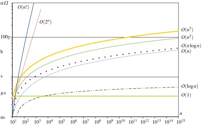

  

  Illustration of the growth of some functions frequently used to express the complexity of an algorithm. The horizontal axis indicates the size of the problem (with exponential growth) and the vertical axis gives the order of magnitude of the computation time (with iterated-exponential growth, from a nanosecond to the expected life of our universe)

• $O(\log n)$: logarithmic; the base is not provided since O(log_a n) = O(log_b n).

• O(n ^c): fractional power, with 0 < c < 1.

• O(n): linear.

• $O(n \log n)$: linearithmic.

• O(n ²): quadratic.

• O(n ³): cubic.

• O(n ^c): polynomial, with c > 1 constant.

• $O(n^{\log n})$: quasi-polynomial, super-polynomial, sub-exponential.

• O(c ⁿ): exponential, with c > 1 constant.

• O(n!): factorial.

2.3 Basic Complexity Classes

Complexity theory has evolved considerably since the beginning of the 1970s, when Cook showed there is a problem which, if we were able to solve it in polynomial time, then it would allow us to solve many others efficiently, like the traveling salesman, the integer linear programming, the graph coloring, etc. [1].

To achieve this result, it was necessary to formulate a generic problem in mathematical terms, how a computer works, and how computational time can be measured. To simplify this theory as much as possible, the type of problems considered is limited to decision problems .

A decision problem is formalized by a generic problem and a question; the answer should be either “yes” or “no.”

Example of a Generic Problem

Let C = {c ₁, …, c _n} be a set of n cities, integer distances d _ij between the cities c _i and c _j (i, j = 1, …, n), and B an integer bound.

Question

Is there a tour of length not higher than B visiting every city of C? Put differently, we look for a permutation p of the elements 1, 2, …, n such that $d_{p_n, p_1} + \sum _{i = 1}^{n-1}{d_{p_i}, d_{p_{i+1}}} \leqslant B$.

This is the decision version of the traveling salesman problem (TSP for short). The optimization version of the problem seeks to find the shortest possible route that visits each city exactly once and returns to the origin city. This is undoubtedly the best-known combinatorial optimization problem that is intractable.

2.3.1 Encoding Scheme, Language, and Turing Machine

A problem instance can be represented as a text file. We must subsequently use given conventions, for example, put on the first line n, the number of cities, then B, the bound, on the second line, and each of the following line will contain three numbers, interpreted as i, j and d _ij. Put differently, an encoding scheme is used.

We can adopt the formal grammar of language theory, which is similar to those used in compiling techniques. Let Σ be a finite set of symbols or an alphabet. We write Σ ^∗ the set of all strings that can be built with the alphabet Σ. An encoding scheme e for a generic problem π allows describing any instance I of π by a string x ∈ Σ ^∗. For the TSP, I contains n, B and all the d _ij values.

An encoding scheme e for generic problem π partitions the strings of Σ ^∗ into three classes:

• 1. The strings that do not encode a problem instance I of π

• 2. The strings encoding a problem instance I of π for which the answer is “no”

• 3. The strings encoding a problem instance I of π for which the answer is “yes”

This last class is called the language associated with π and e, denoted L(π, e).

In theoretical computer science, or more precisely in automata theory, the computing power of various machine models is studied. Among the simplest automata, there are finite-state automata. They are utilized to design or analyze a communication protocol for instance. Their states are represented by the vertices of a graph and transitions, represented by arcs. Providing an input string, the automaton changes from one state to another according to the symbol of the string being read and associated transitions rules. Since an automaton maintains a finite number of states, this machine possesses a bounded memory.

A slightly more complex model is a push-down automaton, functioning similarly to a finite-state machine, but has a stack. At each step, a symbol of the string is interpreted, as well as the symbol at the top of the stack (if the last is not empty). The automaton changes its state and places a new symbol at the top of the stack. This type of automaton is able to make more complex computations. For instance, it can recognize the strings of a non-contextual language. Hence, it can perform the syntax analysis of a program described by a grammar of type 2. An even more powerful computer model than a stack automaton is the Turing machine.

Deterministic Turing Machine

To mathematically represent how a computer works, Alan Turing imagined a fictive machine (there were no computers in 1936) whose operations can be modeled by a transition function. This machine is able to implement all the usual algorithms. It is able to recognize a string generated by a general grammar of type 0 in a finite time. Figure 1.6 illustrates such a machine, composed of a program that controls the scrolling of a magnetic tape and a read/write head.

Fig. 1.6

Schematic representation of a deterministic Turing machine, which allows modeling and formalizing a computer

A program for a deterministic Turing machine is specified by:

• 1. A tape alphabet Γ—the set of symbols that can be written on the tape. Γ contains at least Σ, the set of symbols that encodes a decision problem instance, the special blank symbol b not belonging to Σ and eventually other control symbols.

• 2. A set of states Q, containing at least q ₀, the initial state, q _Y, the final state indicating that the answer to the instance is “yes” and q _N, the final state indicating that the answer is “no.”

• 3. A transition function δ : Q ∖{q _Y, q _N}× Γ  →  Q × Γ ×{−1, 1}.

This function represents the actions to be performed by the machine when it is in a certain state and reads a certain symbol. A Turing machine works as follows: its initial state is q ₀, the read/write head is positioned on cell 1; the tape contains the string x ∈ Σ ^∗ in cells 1 through |x| and b for all other cells. Let q be the current state of the machine, σ the symbol read from the tape and (q′, σ′, Δ) = δ(σ, q). One step of the machine consists in:

• Replacing σ by σ′ in the current cell

• Moving the head one cell to the left if Δ = −1 or one cell to the right if Δ = 1

• Changing the internal state to q′

The machine stops either in state q _Y or in state q _N. This is the reason why the transition function δ is only defined for nonfinal states of the machine.

Although very simple, a Turing machine can conceptually represent everything that happens in a common computer. This is not the case for simpler machines, like the finite-state automaton (which head always moves toward the same direction) or the push-down automaton.

Example of a Turing Machine Program

Let M = (Γ, Σ, Q, δ) be a Turing Machine program:

Tape alphabet: Γ = {0, 1, b}

Input alphabet: Σ = {0, 1}

Set of states: Q = {q ₀, q ₁, q ₂, q ₃, q _Y, q _N}

Transition function δ: given in Table 1.1

Table 1.1 Specification of the transition function δ of a Turing machine

2.3.2 Class P of Languages

The class P (standing for polynomial) contains the problems considered easy: those for which an algorithm can solve the problem with a number of steps polynomially limited to the instance data size (the length of the string x initially written on the tape). More formally, this class is defined as follows: we say the machine M accepts x ∈ Σ ^∗ if and only if M stops in the state q _Y. The language recognized by M is the set of strings x ∈ Σ ^∗ such that M accepts x. We can verify that the language recognized by the machine given by the program in Table 1.1 is the strings encoding a binary number divisible by 4.

An algorithm is a program that stops for any string x ∈ Σ ^∗. The computational time of an algorithm is the number of steps performed by the machine before it stops. The complexity of a program M is the largest computational time T _M(n) required by the machine to stop, whatever the string x of length n initially written on the tape is. A deterministic Turing machine program is in polynomial time if there is a polynomial p such that $T_M(n) \leqslant p(n)$

The class P of languages includes all the languages L such that there is a program for deterministic Turing machine recognizing L in polynomial time. By abuse of language, we say the problem π belongs to the class P if the language associated with π and with an encoding scheme e (unspecified but supposed to be reasonable) belongs to P. When we use the expression “there is a program”; we know this program exists, but without necessarily knowing how to code it. Conversely, if we are aware of an algorithm—not necessarily the best one—running in polynomial time for this problem, then the problem belongs to the complexity class P.

2.3.3 Class NP of Languages

Informally, the class NP (standing for nondeterministic polynomial) of languages includes all the problems for which we can verify in polynomial time that a given solution produces the answer “yes.” For a problem to be part of this class, the requirements are looser than for the class P. Indeed, it is not required to be able to find a solution in polynomial time but only to be able to verify the correctness of a given solution in polynomial time. Practically, this class contains intractable problems, for which we are not aware of a polynomial time solving algorithm.

To formalize this definition, theoretic computer scientists have imagined a new type of theoretical computer, the nondeterministic Turing machine, which has no material equivalent in our real world. Conceptually, this machine is composed of a module that guesses the solution of the problem and writes it into the negative index cells of the tape (see Fig. 1.7). This artifice allows us to overcome our ignorance of an efficient algorithm to solve the problem: the machine just does the job and guesses the solution.

Fig. 1.7

Schematic representation of a nondeterministic Turing machine. This machine allows formalizing the NP class, but does not exist in the real world

The specification of a program for a nondeterministic Turing machine is identical to that of a deterministic one. Initially, the machine is in state q ₀, the tape contains the string x encoding the problem in cells 1 to |x|, and the program is idle. At that time, a guessing phase starts during which the module writes random symbols in the negative cells and stops arbitrarily. Next, the machine’s program is activated, and it works as a deterministic Turing machine.

With such a machine, it is obvious that a given string x can generate various computations, because of the nondeterministic character of the guessing phase. The machine can end in q _N state even if the problem includes a feasible solution. Different runs with various computational times can end in the q _Y state. But the machine cannot end in the state q _Y for a problem that has no solution.

By definition, the language L _M recognized by the nondeterministic machine M is the set of strings x ∈ Σ ^∗ such that there is at least one computation for which the string x is accepted. The computation time T _M(n) is the minimum number of steps taken by the machine to accept a string x of length n. The number of steps in the guessing phase is not counted. The complexity of a program is defined in a similar way to that of a deterministic machine.

The class NP of languages is formally defined as the set of languages L for which there exists a program M for a nondeterministic Turing machine so that M recognizes L in polynomial time. We insist on the fact that the name of this class comes from “nondeterministic polynomial” and not from “non-polynomial.”

Polynomial Transformation

The notion of polynomial transformation of an initial problem into a second one is fundamental in the theory of complexity, because it is of substantial help for problem classification. Indeed, if we are able to efficiently solve the second problem—or, for intractable problems, if we were able to efficiently solve the second problem—and we know an inexpensive way of transforming the initial problem into the second one, then we can also effectively solve the initial problem.

Formally, a first language $L_1 \subset \varSigma _1^*$ can be polynomially transformed into a second language $L_2 \subset \varSigma _2^*$ if there is a function $f : \varSigma _1^* \rightarrow \varSigma _2^*$ that can be evaluated in polynomial time by a deterministic Turing machine, such that, for all problem instance $x \in \varSigma _1^*$ with “yes” answer, f(x) is an instance of the second problem with “yes” answer. Such a polynomial transformation is written $L1 \varpropto L2$. We write L ₁ ∝_T(n) L ₂ if we want to specify the time T(n) required to evaluate f.

Figure 1.8 illustrates the principle of a polynomial transformation. When transforming a problem into another one, it is solely concerned about the complexity of the evaluation of the f function and the answers “yes-no” of both instances should be the same. The complexity of solving instance 2 or that of the decoding of a solution of instance 1 from that of instance 2 is not required.

Fig. 1.8

Polynomial transformation of Problem ₁ to Problem ₂ in time T(n). The theory only requires to be able to carry out the operations represented with solid line arrows

Example of Polynomial Transformation

Let us consider the problem of finding a Hamiltonian cycle in a graph (a cycle passing only once by all the vertices of the graph before returning to the starting vertex) and the traveling salesman problem. The last is to answer the question: is there a tour of total length no more than B? The f function to transform the Hamiltonian cycle into an instance of a traveling salesman builds a complete network on the same set of vertices as for the graph. In the network, it associates a weight of zero with the existing edges of the graph and a weight of one with the edges that are missing in the graph. The bound B is zero.

There is a solution of length 0 to the traveling salesman if and only if there is a Hamiltonian cycle in the initial graph. We deduce the Hamiltonian cycle can be transformed into a traveling salesman problem. It should be noted that the opposite is not necessarily true.

2.3.4 Class NP-Complete

A problem π belongs to the class NP-complete if π belongs to NP and every problem of NP can be polynomially transformed into π.

Starting from the definition of a polynomial transformation and noting the composition of two polynomials is still a polynomial, we have the following properties:

• If π is NP-complete and π can be solved in polynomial time, then P = NP.

• If π is NP-complete and π does not belong to P, then P ≠ NP.

• If π ₁ polynomially transforms into π ₂ and π ₂ polynomially transforms into π ₃, then π ₁ polynomially transforms into π ₃.

• If π ₁ is NP-complete, π ₂ belongs to NP and π ₁ polynomially transforms into π ₂, then π ₂ is NP-complete.

No NP-complete problem that can be solved in polynomial time is known. It is conjectured that no such problem exists, hence it is assumed that P ≠ NP. The latter property listed above is frequently exploited to show that a problem π ₂, of a priori unknown complexity, is NP-complete. For this, a problem π ₁ belonging to the NP-complete class is chosen, and a polynomial transformation of any instance of π ₁ into an instance of π ₂ is exhibited.

The NP-complete class definition presented above is purely theoretical. Maybe, this class is just an empty one! Therefore, it should be asked whether there exists at least one problem belonging to this class or not? It is indeed far from obvious to find a “universal” problem of NP such that all the other problems of NP can be polynomially transformed into this problem. It is not possible to imagine what all the problems of NP are and even less to find a transformation for each of them into the universal problem. However, such a problem exists, and the first that was shown to be NP-complete was the satisfiability problem.

Satisfiability

Let u ₁, …u _m be a set of Boolean variables. A literal is a variable or its negation. A (disjunctive) clause is a finite collection of literals connected together with logical “or” (∨). A clause is false if and only if all its literals are false. A satisfiability problem is a collection of clauses connected together with the logical “and” (∧). An instance of satisfiability is feasible if there are assignments of values to the Boolean variables such that all the clauses are simultaneously true.

For instance, the satisfiability problem $(u_1 \lor \overline {u_2}) \land (\overline {u_1} \lor u_2)$ is feasible. However, $(u_1 \lor u_3) \land (u_1 \lor \overline {u_3}) \land (\overline {u_1}) \land (u_2)$ is not a feasible instance. The graph coloring problem modeled with a Boolean formula given at the very beginning of this chapter is a satisfiability problem.

In the early 1970s, Cook shows that satisfiability is NP-complete. From this result, it was quite easy to show that many others also belong to the class NP-complete, using the principle stated in the remark above. In the late 1970s, several hundred problems were shown to be NP-complete.

Below is the example of the polynomial transformation of satisfiability into the stable set problem. Since any problem of NP can be transformed into satisfiability and any satisfiability instance can be transformed into the stable set, the latter is NP-complete.

Stable Set

Data: a graph G = (V, E) and k an integer. Question: Is there a subset V ′⊆ V, |V ′| = k such that ∀i, j ∈ V ′, (i, j)∉E (i.e., a subset of k nonadjacent vertices)?

Satisfiability is transformed into stable set as follows:

• A vertex is associated with all literals of each clauses.

• For each clause, a complete subgraph is created.

• Incompatible literals-vertices are connected together (a variable and its negation).

• A stable set of k vertices is searched in this graph, where k is the number of clauses.

Such a transformation is illustrated in Fig. 1.9 for a little instance with three literals and three clauses.

Fig. 1.9

Polynomial transformation of satisfiability instance: $(\bar {x} \lor y \lor \bar {z}) \land (x \lor \bar {y}) \land (y \lor z)$ to a stable set

Example of Unknown Complexity Problems

At this time, thousands of problems have been identified to be either in P or in NP-complete class. A number of them are not yet classified more precisely than in NP. Here are two examples of such problems:

• In a soccer league, each team play each other once. The winning team receives three points. The losing team receives zero points. In case of a tie, each team receives one point. Given a series of scores for each team, can this series be the result obtained at the end of a championship? Note: if the winner receives only two points, then there is a polynomial algorithm to answer this question.

• Is it possible to orient the edges of a graph so that it is strongly connected and that each vertex has an odd indegree?

2.3.5 Strongly NP-Complete Class

In some cases, NP-complete problem instances are well solved by means of ad hoc algorithms. For instance, dynamic programming can manage knapsack problems (see Sect. 2.5.3) with numerous items. A condition for these instances to be easily solved is that the largest number appearing in the data is limited. For the knapsack problem, this number is its volume. On the contrary, other problems cannot be solved effectively, even if the value of the largest number appearing in the problem is limited.

We are addressing a number problem if there is no polynomial p(n) such that the largest number M appearing in the data of an instance of size n is bounded by p(n). The partition of a set into two subsets of equal weight or the traveling salesman are, therefore, problems on numbers because, if we add one bit to the size of the problem, M can be multiplied by two. Therefore, for these problems, M can be in O(2ⁿ), which is not polynomial.

We say an algorithm is pseudo-polynomial if it runs in a time bounded by a polynomial depending on the size n of the data and the largest number M appearing in the problem. The partition of a set into two subsets of equal weight is an NP-complete problem for which there is a simple pseudo-polynomial algorithm.

Instance of a Partition Problem

Is it possible to divide the set {5, 2, 1, 6, 4} into two subsets of equal weights? The sum of the weights for this partition problem instance is 18. Therefore, we look for two subsets of weight 9.

To solve this problem, we create an array of n rows, where n is the number of elements in the set, and M = 9 columns, where M is half of the sum of the element weights. We eventually fill the cells of this table with × by proceeding line by line. Using only the first element, of weight 5, we manage to create a subset of weight 0 (if we do not take this element) or a subset of weight 5 (taking it). Hence, we place × in the columns 0 and 5 of the first line.

Using only the first two elements, it is possible to create subsets whose weight is the same as with a single element (by not taking the second element). In the second line of the table, we can copy the × of the previous line. By taking the second element, we can create subsets of weights 2 and 7. Hence, we put × where we put them for the previous line but shifted by the weight of the second element (here: 2).

The process is then repeated until all the elements have been considered. As soon as there is a × in the last column, it means it is possible to create a subset of weight M. This is the case for this instance. One solution is {2, 1, 6}{5, 4}. The complexity of the algorithm is O(M ⋅ n), which is indeed polynomial in n and M.

	Sum of the weights
Element	0	1	2	3	4	5	6	7	8	9
5	×					×
2	×		×			×		×
1	×	×	×	×		×	×	×	×
6	×	×	×	×		×	×	×	×	×
4	×	×	×	×	×	×	×	×	×	×

Let π be a number problem and π _p(n) ⊂ π, the subset restricted to instances for which $M \leqslant p(n)$. The set π _p(n) contains only instances of π with “small” numbers. It is said that π is strongly NP-complete if and only if there is a polynomial p(n) such that π _p(n) is NP-complete.

With this definition, a strongly NP-complete problem cannot be solved in pseudo-polynomial time if the class P is different from the class NP. Thus, the traveling salesman problem is strongly NP-complete because the Hamiltonian cycle can polynomially transform into the traveling salesman with a distance matrix containing only 0s or 1s. Since the Hamiltonian cycle is NP-complete, traveling salesman instances involving only small numbers are also NP-complete.

Conversely, the problems that can be solved with dynamic programming, like the knapsack or the partition problem, are not strongly NP-complete. Indeed, if the sum of the weights of the n elements of a partition problem is bounded by a polynomial p(n), the algorithm presented above has complexity in O(n ⋅ p(n)) which is polynomial.

2.4 Other Complexity Classes

Countless other complexity classes have been proposed. Among those which are most frequently encountered in the literature and which can be described intuitively, we can cite:

NP-Hard:

The problems considered above are decision problems, not optimization ones. With a dichotomy algorithm, we can easily solve the optimization problem associated with a decision problem. A problem is NP-hard if any problem of NP can transform into this problem in polynomial time. Unlike the NP-complete class, we do not force the latter to be part of NP. Thus, an optimization problem whose decisional version is NP-complete falls into the category of NP-hard problems.

P-SPACE:

The problems that can be solved with a machine whose memory is limited by a polynomial in the data size belong to the class P-SPACE. No limit is imposed here on the computational time, which can be exponential. Thus, all the problems of NP are in P-SPACE because we can design exhaustive enumeration algorithms that do not require too much memory. An example of a problem in this class is to determine whether a two-player deterministic game is unfair, i.e., if player B is sure to lose if player A does not make mistakes. This problem is unlikely to be part of the class NP, because it is hard to imagine that a concise certificate can be given for solutions to problems of this class.

Class L :

The problems which can be solved with a machine whose working memory is bounded by a polynomial in the size of the data—by disregarding the space necessary for the storage of the problem data—are part of the class L. This class includes problems of finding elements in databases whose size does not fit in the computer RAM.

Class NC :

The class NC contains the problems that can be solved in poly-logarithmic time on a machine including a polynomial number of processors. The problems of this class can therefore be solved in parallel in a shorter time than that which is needed to sequentially read the data. The sorting of the elements of an array falls under the NC class.

Few results have been established regarding the relationships between these various complexity classes. With the exception of the obvious inclusions in the broad sense L ⊆ P ⊆ NP ⊆ NP-complete ⊆ P-SPACE and NC ⊆ P, the only strict inclusion established is L ≠  P-SPACE. It is conjectured that P ≠ NP. This is a millennium problem. A deeper presentation of this topic can be found in [2].

Problems

1.1

Draw Five Segments

Try to draw five segments of lines on the plane so that each segment cuts exactly three others. Formalize this problem in terms of graphs.

1.2

O Simplification

Simplify the following expressions:

• O(n ⁵ + 2ⁿ)

• $O(5^n + 2^{2^n})$

• Ω(n ² ⋅ n! + (n + 2)!)

• $\varOmega (n \log (\log (n)) + 23 n)$

• $O(n^{\log (n)} + n^{5 + cos(n)})$

• $O(n \log (n) + n^{3 - 2\cdot sin(n)})$

1.3

Turing Machine Program

Write a deterministic Turing machine program that recognizes if the substring ane is written on the tape. The input alphabet is Σ = {a, c, e, n}. Specify the tape alphabet Γ, the state set Q and the transition function δ.

1.4

Clique is NP-Complete

Show that finding a clique of a given size in a graph is NP-complete.

1.5

Asymmetric TSP to Symmetric TSP

Show that the asymmetric traveling salesman problem—the distance from city i to j can be different from the distance from city j to i—can be polynomially transformed into the symmetric TSP by doubling the number of cities.

References

Cook, S.A.: The complexity of theorem-proving procedures. In: Proceedings of the Third Annual ACM Symposium on Theory of Computing, pp. 151–158. ACM, New York (1971). https://doi.org/10.1145/800157.805047
Garey, M.R., Johnson, D.S.: Computers and Intractability — A Guide to the Theory of NP-Completeness. W. H. Freeman, New York (1979)
Author information
Authors and Affiliations
Rights and permissions
Open Access This chapter is licensed under the terms of the Creative Commons Attribution 4.0 International License (http://creativecommons.org/licenses/by/4.0/), which permits use, sharing, adaptation, distribution and reproduction in any medium or format, as long as you give appropriate credit to the original author(s) and the source, provide a link to the Creative Commons license and indicate if changes were made.
The images or other third party material in this chapter are included in the chapter's Creative Commons license, unless indicated otherwise in a credit line to the material. If material is not included in the chapter's Creative Commons license and your intended use is not permitted by statutory regulation or exceeds the permitted use, you will need to obtain permission directly from the copyright holder.
Copyright information
© 2023 The Author(s)
About this chapter
Cite this chapter
Taillard, É.D. (2023). Elements of Graphs and Complexity Theory. In: Design of Heuristic Algorithms for Hard Optimization. Graduate Texts in Operations Research. Springer, Cham. https://doi.org/10.1007/978-3-031-13714-3_1
Download citation
DOI: https://doi.org/10.1007/978-3-031-13714-3_1
Published:
Publisher Name: Springer, Cham
Print ISBN: 978-3-031-13713-6
Online ISBN: 978-3-031-13714-3
eBook Packages: Business and ManagementBusiness and Management (R0)