
Abstract
The core of this book are deep learning methods and neural networks. This chapter considers deep feed-forward neural (FN) networks. We introduce the generic architecture of deep FN networks, and we discuss universality theorems of FN networks. We present network fitting, back-propagation, embedding layers for categorical variables and insurance-specific issues such as the balance property in network fitting, as well as network ensembling to reduce model uncertainty. This chapter is complemented by many examples on non-life insurance pricing, but also on mortality modeling, as well as tools that help to explain deep FN network regression results.
You have full access to this open access chapter, Download chapter PDF
In the sequel, we introduce deep learning models. In this chapter these deep learning models will be based on fully-connected feed-forward neural networks. We present these networks as an extension of GLMs. These networks perform feature engineering themselves. We discuss how networks achieve this, and we explain how networks are used for predictive modeling. There is a vastly growing literature on deep learning with networks, the classical reference is the book of Goodfellow et al. [166], but also the numerous tutorials around the open-source deep learning libraries TensorFlow [2], Keras [77] or PyTorch [296] give an excellent overview of the state-of-the-art in this field.
7.1 Deep Learning and Representation Learning
In Chap. 5 on GLMs, we have been modeling the mean structure of the responses Y , given features x, by the following regression function, see (5.6),
The crucial assumption has been that the regression function (7.1) provides a reasonable functional description of the expected value \({\mathbb E}_{\theta (\boldsymbol {x})}[Y]\) of datum (Y, x). As described in Sect. 5.2.2, this typically requires manual feature engineering of x, bringing feature information into the right structural form.
In contrast to manual feature engineering, deep learning aims at performing an automated feature engineering within the statistical model by massaging information through different transformations. Deep learning uses a finite sequence of functions (z (m))1≤m≤d, called layers,
of (fixed) dimensions \(q_{m} \in {\mathbb N}\), 1 ≤ m ≤ d, and initialization q 0 = q being the dimension of the (raw) feature information \(\boldsymbol {x}\in \mathcal {X} \subset \{1\} \times {\mathbb R}^q\). Each of these layers presents a new representation of the features, that is, after layer m we have a q m-dimensional representation of the raw feature \(\boldsymbol {x} \in \mathcal {X}\)

Note that the first component is always identically equal to 1. For this reason we call the representation \(\boldsymbol {z}^{(m:1)}(\boldsymbol {x}) \in \{1\}\times {\mathbb R}^{q_m}\) of x to be q m-dimensional.
Deep learning now assumes that we have \(d \in {\mathbb N}\) appropriate transformations (layers) z (m), 1 ≤ m ≤ d, such that z (d:1)(x) provides a suitable q d-dimensional representation of the raw feature \(\boldsymbol {x} \in \mathcal {X}\), that then enters a GLM
with link function \(g:\mathcal {M}\to {\mathbb R}\) and regression parameter \(\boldsymbol {\beta } \in {\mathbb R}^{q_d+1}\). This regression architecture is called a feed-forward network of depth \(d \in {\mathbb N}\) because information x is processed in a directed acyclic (feed-forward) path through the d layers z (1), …, z (d) before entering the final GLM.
Each layer z (m) involves parameters. Successful deep learning simultaneously fits these parameters as well as the regression parameter β to the available learning data \(\mathcal {L}\) so that we obtain an optimal predictive model on the test data \(\mathcal {T}\). That is, the learned model should optimally generalize to unseen data, we refer to Chap. 4 on predictive modeling. Thus, the process of optimal representation learning is also part of the model fitting procedure. In contrast to GLMs, the resulting log-likelihood functions are non-concave in their parameters because, typically, each layer involves non-linear transformations. This makes model fitting a challenge. State-of-the-art model fitting in deep learning uses variants of the gradient descent algorithm which we have already met in Sect. 6.2.4.
Remark 7.1. Representation learning x↦z (d:1)(x) is closely related to Mercer’s kernel [272]. If we have a portfolio with features x 1, …, x n, we obtain a Mercer’s kernel by considering the matrix
In many regression problems it can be shown that one can equivalently work with the design matrix  or with Mercer’s kernel \(\mathbf {K} \in {\mathbb R}^{n\times n}\). Mercer’s kernel does not require the full knowledge of the learned representations z
(d:1)(x
i), but it suffices to know the discrepancies between z
(d:1)(x
i) and z
(d:1)(x
j) measured by the scalar products K(x
i, x
j). This is also closely related to the cosine similarity in word embeddings, see (10.11). This approach then results in replacing the search for an optimal representation learning by a search of the optimal Mercer’s kernel for the given data; this is called the kernel trick in machine learning.
or with Mercer’s kernel \(\mathbf {K} \in {\mathbb R}^{n\times n}\). Mercer’s kernel does not require the full knowledge of the learned representations z
(d:1)(x
i), but it suffices to know the discrepancies between z
(d:1)(x
i) and z
(d:1)(x
j) measured by the scalar products K(x
i, x
j). This is also closely related to the cosine similarity in word embeddings, see (10.11). This approach then results in replacing the search for an optimal representation learning by a search of the optimal Mercer’s kernel for the given data; this is called the kernel trick in machine learning.
7.2 Generic Feed-Forward Neural Networks
Feed-forward neural (FN) networks use special layers z (m) in (7.2)–(7.3), whose components are called neurons. This is discussed and studied in detail in this section.
7.2.1 Construction of Feed-Forward Neural Networks
FN networks are regression functions of type (7.3) where each neuron \(z_j^{(m)}\), 1 ≤ j ≤ q
m, of the layers  , 1 ≤ m ≤ d, has the structure of a GLM; the first component \(z_0^{(m)}=1\) always plays the role of the intercept and does not need any modeling.
A first important choice is the activation function \(\phi : {\mathbb R} \to {\mathbb R}\) which plays the role of the inverse link function g −1. To perform non-linear representation learning, this activation function should be non-linear, too. The most popular choices of activation functions are listed in Table 7.1.
The first three examples in Table 7.1 are smooth functions with simple derivatives, see the last column of Table 7.1. Having simple derivatives is an advantage in gradient descent algorithms for model fitting. The derivative of the ReLU activation function for x ≠ 0 is given by the step function activation, and in 0 one typically considers a sub-gradient. We briefly comment on these activation functions.
-
We are mainly going to use the hyperbolic tangent activation function
$$\displaystyle \begin{aligned} x~\mapsto~\tanh (x)~=~\frac{e^{x}-e^{-x}}{e^{x}+e^{-x}} ~=~ 2\left(1+e^{-2x}\right)^{-1}-1 ~\in~ (-1,1). \end{aligned}$$Figure 7.1 illustrates the hyperbolic tangent activation function.
Fig. 7.1 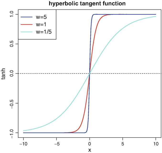
Hyperbolic tangent activation function \(x \mapsto \tanh (wx) \in (-1,1)\) for (fixed) weights w ∈{1∕5, 1, 5} and x ∈ (−10, 10)
The hyperbolic tangent activation function is anti-symmetric w.r.t. the origin with range (−1, 1). This anti-symmetry and boundedness is an advantage in fitting deep FN network architectures. For this reason we usually prefer the hyperbolic tangent over other activation functions.
-
The sigmoid activation function corresponds to the logistic function that was used in the Bernoulli and the categorical EFs, see Sects. 2.1.2 and 5.7. The sigmoid activation function can be obtained from the hyperbolic tangent activation function by setting \(\phi (x)=(\tanh (x/2)+1)/2\).
-
The step function activation is not really used in applications. However, it allows for nice interpretations, and it links FN networks to the theory of regression and classification trees (CARTs); see Breiman et al. [54] for CARTs.
-
The exponential activation function is a nice differentiable choice whenever the range should be one-sided bounded.
-
The ReLU activation function is also called hinge function or ramp function. This is the preferred choice in the machine learning community. However, typically, we will not use it because in our experience it is less robust in fitting compared to the hyperbolic tangent activation function. This may be for two reasons, firstly, the ReLU activation is unbounded, and secondly, it is identically equal to zero for x < 0, which implies that there is no sensitivity in negative choices of x.

A FN layer with activation function ϕ is a mapping

having neurons for 1 ≤ j ≤ q m
with given network weights \(\boldsymbol {w}^{(m)}_j=(w^{(m)}_{l,j})_{0\le l \le q_{m-1}} \in {\mathbb R}^{q_{m-1}+1}\).
Interpretation
Every neuron \(\boldsymbol {z}\mapsto z_j^{(m)}(\boldsymbol {z})\) describes a GLM regression function with link function ϕ −1 and regression parameter \(\boldsymbol {w}^{(m)}_j \in {\mathbb R}^{q_{m-1}+1}\) for features \(\boldsymbol {z} \in \{1\}\times {\mathbb R}^{q_{m-1}}\). These GLM regression functions can be interpreted as data compression, i.e., in each neuron the q m−1-dimensional feature z is projected to a real number \(\langle \boldsymbol {w}^{(m)}_j, \boldsymbol {z} \rangle \in {\mathbb R}\) which is then (non-linearly) activated by ϕ. Since this leads to a substantial loss of information, we perform this procedure of data compression q m times in FN layer z (m), so that each neuron in \((z_j^{(m)}(\boldsymbol {z}))_{1\le j \le q_m}\) represents a different projection of input z. Choosing suitable weights \(\boldsymbol {w}^{(m)}_j\) will allow us to extract the crucial feature information from z to receive good explanatory variables for the regression task at hand.
A FN network of depth \(d \in {\mathbb N}\) is obtained by composing d FN layers z (1), …, z (d) to receive the mapping
Choosing a strictly monotone and smooth link function g and a regression parameter \(\boldsymbol {\beta } \in {\mathbb R}^{q_d+1}\) we receive the FN network regression function
This FN network regression function (7.8) has a network parameter
 of dimension
In Fig. 7.2 we illustrate a FN network of depth d = 3, FN layers of dimensions (q 1, q 2, q 3) = (20, 15, 10) and input dimension q 0 = 40.Footnote 1 This gives us a network parameter \(\boldsymbol {\vartheta } \in {\mathbb R}^r\) of dimension r = 1′306. On the left-hand side we have the raw features \(\boldsymbol {x} \in \mathcal {X}\subset \{1\}\times {\mathbb R}^{q_0}\), these are processed through the three FN layers, where the black circles illustrate the neurons \(z_j^{(m)}\). The third FN layer z (3) has dimension q 3 = 10 providing the learned representation \(\boldsymbol {z}^{(3:1)}(\boldsymbol {x})\in \{1\}\times {\mathbb R}^{q_3}\) of x. This is used in the final GLM step (7.8) in the green box of Fig. 7.2.

FN network of depth d = 3, with number of neurons (q 1, q 2, q 3) = (20, 15, 10) and input dimension q 0 = 40. This gives us a network parameter \(\boldsymbol {\vartheta } \in {\mathbb R}^r\) of dimension r = 1′306
Remarks 7.2.
-
One distinguishes between FN networks of depth d = 1, called shallow networks, and FN networks of depth d > 1, called deep networks. In this sense, deep learning means that we learn suitable feature representations through multiple FN layers d > 1. We come back to this in Sect. 7.2.2, below. Remark that some people would only call a network deep if d ≫ 1, here d > 1 will be chosen for the definition of deep (which is also a precise definition).
-
There are two ways of receiving a GLM. If we have a (trivial) FN network of depth d = 0, this naturally corresponds to a GLM, see Fig. 7.2. In that case, one works with the original features \(\boldsymbol {x} \in \mathcal {X}\) in (7.8). The second way of receiving a GLM is given by choosing the identity function as activation function ϕ(x) = x. This implies that x↦z (d:1)(x) = A x is a linear function for some matrix \(A \in {\mathbb R}^{(q_d+1) \times (q+1)}\) and, henceforth, we receive a GLM.
-
Under the above interpretation of the representation learning structure (7.7), we may also give a different intuition for the FN layers. Typically, we expect that the first FN layers decompose feature information x into bits and pieces, which are then recomposed in a suitable way for the prediction task. In this sense, we typically choose a larger dimension for the early FN layers otherwise we may lose too much information already from the very beginning.
-
The neural network introduced in (7.7) is called FN network because the signals propagate from one layer to the next (directed acyclic graph). If the network has loops it is called a recurrent neural (RN) network. RN networks have been applied very successfully in image and speech recognition, for instance, long short-term memory (LSTM) networks are very useful for time-series analysis. We study RN networks in Chap. 8, below. A third type of neural networks are convolutional neural (CN) networks which are very successfully applied to image recognition because they are capable to detect similar structures at different places in images, i.e., CN networks learn local representations. We will discuss CN network architectures in Chap. 9, below.
-
The generic FN network architecture (7.8) can be complemented by drop-out layers, normalization layers, skip connections, embedding layers, etc. Such layers are special purpose layers, for instance, taking care of over-fitting. We introduce and discuss these below.
-
The regression function (7.8) has a one-dimensional output for regression modeling. Of course, categorical classification can be done completely analogously by choosing a link function g suitable for classification, see Sect. 5.7. A similar approach also works if, for instance, we want to model simultaneously the mean and the dispersion of the data with a two-dimensional output function g −1.
7.2.2 Universality Theorems
The use of FN networks for representation learning is motivated by the so-called universality theorems which say that any compactly supported continuous (regression) function can be approximated arbitrarily well by a suitably large FN network. As such, we can understand the FN network framework as an approximation tool which, of course, is useful far beyond statistical modeling. In Chapter 12 we give some proofs of selected universality statements to illustrate the flavor of such results. In particular, Cybenko [86], Hornik et al. [192], Hornik [191], Leshno et al. [247], Park–Sandberg [293, 294], Petrushev [302] and Isenbeck–Rüschendorf [198] have shown (under mild conditions on the activation function) that shallow FN networks can approximate any compactly supported continuous function arbitrarily well (in supremum norm or in L 2-norm), if we allow for an arbitrary number of neurons \(q_1\in {\mathbb N}\) in the single FN layer. Roughly speaking, such a result for shallow FN networks holds true if and only if the chosen activation function is non-polynomial, see Leshno et al. [247]. Such results are proved either by algebraic methods of Stone–Weierstrass type or by Wiener–Tauberian denseness type arguments. Moreover, approximation results are studied in Barron [25, 26], Yukich et al. [399], Makavoz [262], Pinkus [303] and Döhler–Rüschendorf [108].
The above stated universality theorems say that shallow FN networks are sufficient from an approximation point of view. Nevertheless, we will mainly use deep (multiple layers) FN networks, below. These have better convergence properties to given function classes because they more easily promote interactions in feature components compared to shallow ones. Such questions have been studied, e.g., by Elbrächter et al. [120], Kidger–Lyons [215], Lu et al. [260] or Cheridito et al. [75]. For instance, Elbrächter et al. [120] compare finite-depth wide networks to finite-width deep networks (under the choice of the ReLU activation function), and they conclude that for many function classes deep networks lead to exponential approximation rates, whereas shallow networks only provide polynomial approximation rates at the same number of network parameters. This motivates to consider sufficiently deep FN networks for representation learning because these typically have a better approximation capacity compared to shallow ones.
We motivate this by two simple examples. For this motivation we use the step function activation  . If we have the step function activation, each neuron partitions \({\mathbb R}^{q_{m-1}}\) along a hyperplane, i.e.,

For a shallow FN network we can study the question of the maximal complexity of the resulting partition of the feature space \(\mathcal {X} \subset \{1\}\times {\mathbb R}^{q_0}\) when considering q 1 neurons (7.9) in the single FN layer z (1). Zaslavsky [400] proved that q 1 hyperplanes can partition the Euclidean space \({\mathbb R}^{q_0}\) in at most
This number (7.10) can be seen as a maximal upper complexity bound for shallow FN networks with step function activation. It grows exponentially for q 1 ≤ q 0, and it slows down to a polynomial growth for q 1 > q 0. Thus, the complexity of shallow FN networks grows comparably slow as the width q 1 of the network exceeds q 0, and therefore we often need a huge network to receive a good approximation.
This result (7.10) should be contrasted to Theorem 4 in Montúfar et al. [280] who give a lower bound on the complexity of regression functions of deep FN networks (under the ReLU activation function). Assume q m ≥ q 0 for all 1 ≤ m ≤ d. The maximal complexity is bounded below by
If we choose as an example a FN network with fixed width q m = 4 for all m ≥ 1 and an input of dimension q 0 = 2, we receive from (7.11) a lower bound of
Thus, we have an exponential growth in depth d →∞. This contrasts the polynomial complexity growth (7.10) of shallow FN networks.
Example 7.3 (Shallow vs. Deep Networks: Partitions). We give a second more explicit example that compares shallow and deep FN networks. Choose q 0 = 2 and assume we want to describe a regression function
If we think of a tool box of basis functions to build regression function μ we may want to choose indicator functions x↦χ A(x) ∈{0, 1} for arbitrary rectangles \(A=[x^-_{1},x^+_{1})\times [x^-_{2},x^+_{2}) \subset {\mathbb R}^2\). We show that we can easily construct such indicator functions χ A(x) for given rectangles \(A \subset {\mathbb R}^2\) with FN networks of depth d = 2, but not with shallow FN networks.
For illustrative purposes, we fix a square \(A=[-1/2,1/2)\times [-1/2,1/2) \subset {\mathbb R}^2\), and we want to construct χ A(x) with a network of depth d = 2. This indicator function χ A is illustrated in Fig. 7.3.

Indicator function χ A(x) for square \(A=[-1/2,1/2)\times [-1/2,1/2) \subset {\mathbb R}^2\)

Shallow FN networks with q 1 = 4 (lhs), q 1 = 8 (middle) and q 1 = 64 (rhs)
We choose the step function activation for ϕ and a first FN layer with q 1 = 4 neurons

This FN layer has a network parameter, see also (7.9),
having dimension q 1(q 0 + 1) = 12. For the second FN layer with q 2 = 4 neurons we choose the step function activation and

This FN layer has a network parameter
having dimension q
2(q
1 + 1) = 20. For the output layer we choose the identity link g(x) = x, and the regression parameter  . As a result, we obtain
That is, this network of depth d = 2, number of neurons (q 1, q 2) = (4, 4), step function activation and identity link can perfectly replicate the indicator function for the square A = [−1∕2, 1∕2) × [−1∕2, 1∕2), see Fig. 7.3. This network has r = 37 parameters.
We now consider a shallow FN network with q 1 neurons. The resulting regression function with identity link is given by

where we have used the step function activation  . As in (7.9), each of these neurons leads to a partition of the space \({\mathbb R}^{2}\) with a straight line. Importantly these straight lines go across the entire feature space, and, therefore, we cannot exactly construct the indicator function of Fig. 7.3 with a shallow FN network. This can nicely be seen in Fig. 7.4 (lhs), where we consider a shallow FN network with q
1 = 4 neurons, weights (7.12), and
. As in (7.9), each of these neurons leads to a partition of the space \({\mathbb R}^{2}\) with a straight line. Importantly these straight lines go across the entire feature space, and, therefore, we cannot exactly construct the indicator function of Fig. 7.3 with a shallow FN network. This can nicely be seen in Fig. 7.4 (lhs), where we consider a shallow FN network with q
1 = 4 neurons, weights (7.12), and  .
.

Schematic figure of a loss surface \(\boldsymbol {\vartheta } \mapsto {\mathfrak D}(\boldsymbol {Y}, \boldsymbol {\vartheta })\) from two different angles for a two-dimensional parameter \(\boldsymbol {\vartheta } \in {\mathbb R}^2\)
However, from the universality theorems we know that shallow FN networks can approximate any compactly supported (continuous) function arbitrarily well for sufficiently large q 1. In this example we can introduce additional neurons and let the resulting hyperplanes rotate around the origin. In Fig. 7.4 (middle, rhs) we show this for q 1 = 8 and q 1 = 64 neurons. We observe that this allows us to approximate a circle, see Fig. 7.4 (rhs), and having circles of different sizes at different locations will allow us to approximate the square A considered above. However, of course, this is a much less efficient way compared to the deep FN network (7.13).
Intuitively speaking, shallow FN networks act like additions where we add more and more separating hyperplanes for q 1 →∞ (superposition of basis functions). In contrast to that, going deep allows us to not only use additions but to also use multiplications (composition of basis functions). This is the reason, why we can easily construct the indicator function χ A in the deep case (where we multiply zero’s along the boundary of A), but not in the shallow case. \(\blacksquare \)
7.2.3 Gradient Descent Methods
We describe gradient descent methods in this section. These are used to fit FN networks. Gradient descent algorithms have already been used in Sect. 6.2.4 for fitting LASSO regularized regression models. We will give the full methodological part here, without relying on Sect. 6.2.4.
7.2.3.1 Plain Vanilla Gradient Descent Algorithm
Assume we have independent instances (Y i, x i), 1 ≤ i ≤ n, that follow the same member of the EDF. We choose a regression function
for a strictly monotone and smooth link function g, and a FN network z
(d:1) with network parameter \(\boldsymbol {\vartheta } \in {\mathbb R}^r\). We assume that the chosen activation function ϕ is differentiable. We highlight in the notation that the mean functional μ
𝜗(⋅) depends on the network parameter 𝜗. The canonical parameter of the response Y
i is given by θ(x
i) = h(μ
𝜗(x
i)) ∈ Θ, where h = (κ′)−1 is the canonical link and κ the cumulant function of the chosen member of the EDF. This gives us (under constant dispersion φ) the log-likelihood function, for given data  ,
,
The deviance loss function in this model is given by, see (4.9) and (4.8),
The MLE of 𝜗 is found by either maximizing the log-likelihood function or by minimizing the deviance loss function in 𝜗. This problem cannot be solved in general because of complexity. Typically, the deviance loss function is non-convex in 𝜗 and it may have many local minimums. This is one of the reasons, why we are less ambitious here, and why we just try to find a network parameter \(\widehat {\boldsymbol {\vartheta }}\) which provides a “small” deviance loss \({\mathfrak D}(\boldsymbol {Y}, \widehat {\boldsymbol {\vartheta }})\) for the given data Y . We discuss this further, below, in fact, this is a crucial point in FN network fitting that is related to in-sample over-fitting and, therefore, this point will require a broader discussion.
For the moment, we just try to find a network parameter \(\widehat {\boldsymbol {\vartheta }}\) that provides a small deviance loss \({\mathfrak D}(\boldsymbol {Y}, \widehat {\boldsymbol {\vartheta }})\) for the given data Y . Gradient descent algorithms suggest that we try to step-wise locally improve our current position by changing the network parameter into the direction of the maximal local decrease of the deviance loss function. By assumption, our deviance loss function is differentiable in 𝜗. This allows us to consider the following first order Taylor expansion in 𝜗

This shows that the locally optimal change \(\boldsymbol {\vartheta } \mapsto \widetilde {\boldsymbol {\vartheta }}\) points into the opposite direction of the gradient of the deviance loss function. This motivates the following gradient descent step.
Assume that at algorithmic time \(t \in {\mathbb N}\) we have a network parameter \(\boldsymbol {\vartheta }^{(t)} \in {\mathbb R}^r\). Choose a suitable learning rate ϱ t+1 > 0, and consider the gradient descent update
This gradient descent update gives us the new (smaller) deviance loss at algorithmic time t + 1
Under suitably tempered learning rates (ϱ t)t≥1, this algorithm will converge to a local minimum of the deviance loss function as t →∞ (supposed that we do not get trapped in a saddlepoint).
Remarks 7.4. We give a couple of (preliminary) remarks on the gradient descent algorithm (7.15), more explanation, further derivations, and variants of the gradient descent algorithm will be discussed below.
-
In the applications we will early stop the gradient descent algorithm before reaching a local minimum (to prevent from over-fitting). This is going to be discussed in the next paragraphs.
-
Fine-tuning the learning rate (ϱ t)t is important, in particular, there is a trade-off between smaller and bigger learning rates: they need to be sufficiently small so that the first order Taylor expansion is still a valid approximation, and they should be sufficiently big otherwise the convergence of the algorithm will be very slow because it needs many iterations.
-
The gradient descent algorithm is a first order algorithm, and one is tempted to study higher order approximations, e.g., leading to the Newton–Raphson algorithm. Unfortunately, higher order derivatives are computationally not feasible if the size n of the data
 and the dimension r of the network parameter 𝜗 are large. In fact, even the calculation of the first order derivatives may be challenging and, therefore, stochastic gradient descent methods are considered below. Nevertheless, it is beneficial to have a notion of a second order term. Momentum-based methods originate from approximating the second order terms, these will be studied in (7.19)–(7.20), below.
 -
The gradient descent step (7.15) solves an unconstraint local optimization. Similarly to (6.15)–(6.16) we could change the gradient descent algorithm to a constraint optimization problem, e.g., involving a LASSO constraint that can be solved with the generalized projection operator (6.17).
 and the dimension r of the network parameter 𝜗 are large. In fact, even the calculation of the first order derivatives may be challenging and, therefore, stochastic gradient descent methods are considered below. Nevertheless, it is beneficial to have a notion of a second order term. Momentum-based methods originate from approximating the second order terms, these will be studied in (
7.2.3.2 Gradient Calculation via Back-Propagation
Fast gradient descent algorithms essentially rely on fast gradient calculations of the deviance loss function. Under the EDF setup we have gradient w.r.t. 𝜗
where the last step uses the variance function V (⋅) of the chosen EDF, we also refer to (5.9). The main difficulty is the calculation of the gradient
w.r.t. the network parameter  , and where each FN layer z
(m) involves the weights \(\mathcal {W}^{(m)}=(\boldsymbol {w}_1^{(m)}, \ldots , \boldsymbol {w}_{q_m}^{(m)}) \in {\mathbb R}^{(q_{m-1}+1)\times q_m}\). The workhorse for these gradient calculations is the back-propagation method of Rumelhart et al. [324]. Basically, the back-propagation method is a clever reparametrization of the problem so that the gradients can be calculated more easily. We therefore modify the weight matrices \(\mathcal {W}^{(m)}\) by dropping the first row containing the intercept parameters \(w_{0,j}^{(m)}\), 1 ≤ j ≤ q
m. Define for 1 ≤ m ≤ d + 1
, and where each FN layer z
(m) involves the weights \(\mathcal {W}^{(m)}=(\boldsymbol {w}_1^{(m)}, \ldots , \boldsymbol {w}_{q_m}^{(m)}) \in {\mathbb R}^{(q_{m-1}+1)\times q_m}\). The workhorse for these gradient calculations is the back-propagation method of Rumelhart et al. [324]. Basically, the back-propagation method is a clever reparametrization of the problem so that the gradients can be calculated more easily. We therefore modify the weight matrices \(\mathcal {W}^{(m)}\) by dropping the first row containing the intercept parameters \(w_{0,j}^{(m)}\), 1 ≤ j ≤ q
m. Define for 1 ≤ m ≤ d + 1
where \(w_{j_{m-1},j_{m}}^{(m)}\) denotes component j m−1 of \(\boldsymbol {w}_{j_m}^{(m)}\), and where we set q d+1 = 1 (output dimension) and \(w_{j_d,1}^{(d+1)}=\beta _{j_d}\) for 0 ≤ j d ≤ q d.
Proposition 7.5 (Back-Propagation for the Hyperbolic Tangent Activation). Choose a FN network of depth \(d\in {\mathbb N}\) and with hyperbolic tangent activation function \(\phi (x)=\tanh (x)\).
-
Define recursively
-
initialize q d+1 = 1 and \(\boldsymbol {\delta }^{(d+1)}(\boldsymbol {x})=\mathbf {1}\in {\mathbb R}^{q_{d+1}}\);
-
iterate for d ≥ m ≥ 1
$$\displaystyle \begin{aligned} \boldsymbol{\delta}^{(m)}(\boldsymbol{x})~=~ \mbox{diag}\left(1-\left(z^{(m:1)}_{j_m}(\boldsymbol{x})\right)^2\right)_{1\le j_m\le q_m} \mathcal{W}^{(m+1)}_{(-0)}\, \boldsymbol{\delta}^{(m+1)}(\boldsymbol{x}) ~\in ~{\mathbb R}^{q_m}. \end{aligned}$$
-
-
We obtain for 0 ≤ m ≤ d
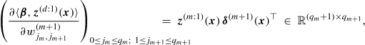
where \(\boldsymbol {z}^{(0:1)}(\boldsymbol {x})=\boldsymbol {x} \in {\mathbb R}^{q_0+1}\) and \(\boldsymbol {w}_1^{(d+1)}=\boldsymbol {\beta } \in {\mathbb R}^{q_d+1}\).

Proof of Proposition 7.5. Choose 1 ≤ m ≤ d and define for the neurons 1 ≤ j m ≤ q m the variables
The learned representation in the m-th FN layer is obtained by activating these variables

For the output we define
The main idea is to calculate the derivatives of 〈β, z (d:1)(x)〉 w.r.t. these new variables \(\zeta _j^{(m)}(\boldsymbol {x})\).
Initialization for m = d + 1
This provides for m = d + 1 and 1 ≤ j d+1 ≤ q d+1 = 1
Recursion for m < d + 1
Next, we calculate the derivatives w.r.t. \(\zeta _{j_d}^{(d)}(\boldsymbol {x})\), for m = d and 1 ≤ j d ≤ q d. They are given by (note q d+1 = 1)
where we have used \(w_{j_d,1}^{(d+1)}=\beta _{j_d}\) and for the hyperbolic tangent activation function ϕ′ = 1 − ϕ 2. Continuing recursively for d > m ≥ 1 and 1 ≤ j m ≤ q m we obtain
Thus, the vectors  are calculated recursively in d ≥ m ≥ 1 with initialization δ
(d+1)(x) = 1 and the recursion
are calculated recursively in d ≥ m ≥ 1 with initialization δ
(d+1)(x) = 1 and the recursion
Finally, we need to show how these derivatives are related to the original derivatives in the gradient descent method. We have for 0 ≤ j d ≤ q d and j d+1 = 1
For 1 ≤ m < d, and 0 ≤ j m ≤ q m and 1 ≤ j m+1 ≤ q m+1 we have
For m = 0, and 0 ≤ l ≤ q 0 and 1 ≤ j 1 ≤ q 1 we have
This completes the proof of Proposition 7.5. □
Remark 7.6. Proposition 7.5 gives the back-propagation method for the hyperbolic tangent activation function which has derivative ϕ′ = 1 − ϕ 2. This becomes visible in the definition of δ (m)(x) where we consider the diagonal matrix
For a general differentiable activation function ϕ this needs to be replaced by, see (7.17),
In the case of the sigmoid activation function this gives us, see also Table 7.1,
_______________________________________________________________
Plain vanilla gradient descent algorithm for FN networks
________________________________________________________________________________________________
-
1.
Choose an initial network parameter \(\boldsymbol {\vartheta }^{(0)} \in {\mathbb R}^r\).
-
2.
Iterate for t ≥ 0 until a stopping criterion is met:
-
(a)
Calculate the gradient \(\nabla _{\boldsymbol {\vartheta }}{\mathfrak D}(\boldsymbol {Y}, \boldsymbol {\vartheta })\) in network parameter 𝜗 = 𝜗 (t) using (7.16) and the back-propagation method of Proposition 7.5 (for the hyperbolic tangent activation function).
-
(b)
Make the gradient descent step for a suitable learning rate ϱ t+1 > 0
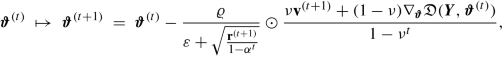
$$\displaystyle \begin{aligned} \boldsymbol{\vartheta}^{(t)} ~\mapsto ~\boldsymbol{\vartheta}^{(t+1)} =\boldsymbol{\vartheta}^{(t)}-\varrho_{t+1} \nabla_{\boldsymbol{\vartheta}}{\mathfrak D}(\boldsymbol{Y}, \boldsymbol{\vartheta}^{(t)}). \end{aligned}$$
-
(a)
__________________________________________________________________
Remark 7.7. The initialization \(\boldsymbol {\vartheta }^{(0)} \in {\mathbb R}^r\) of the gradient descent algorithm needs some care. A FN network has many symmetries, for instance, we can permute neurons within a FN layer and we receive the same predictive model. For this reason, the initial network weights \(\mathcal {W}^{(m)}=(\boldsymbol {w}_1^{(m)}, \ldots , \boldsymbol {w}_{q_m}^{(m)}) \in {\mathbb R}^{(q_{m-1}+1)\times q_m}\), 1 ≤ m ≤ d, should not be chosen with identical components because this will result in a saddlepoint of the corresponding objective function, and gradient descent will not work. For this reason, these weights are initialized randomly either using a uniform or a Gaussian distribution. The former is related to the glorot_uniform initializer in keras,Footnote 2 see (16) in Glorot–Bengio [160]. This initializer scales the support of the uniform distribution with the sizes of the FN layers that are connected by the corresponding weights \(\boldsymbol {w}_j^{(m)}\).
For the output parameter we usually set as initial value  , where \(\widehat {\beta }_0^{(0)}\) is the MLE in the corresponding null model (not considering any features) and transformed to the chosen link g. This choice implies that the gradient descent algorithm starts in the null model, and any decrease in deviance loss can be seen as an improved in-sample loss of using the FN network regression structure over the null model.
7.2.3.3 Stochastic Gradient Descent
The gradient in (7.16) has two parts. We have a vector

and we have a matrix
The gradient of the deviance loss function is obtained by the matrix multiplication
Matrix multiplication can be very slow in numerical implementations if the sample size n is large. For this reason, one typically uses the stochastic gradient descent (SGD) method that does not consider the entire data  simultaneously.
For the SGD method one chooses a fixed batch size \(b \in {\mathbb N}\), and one randomly partitions the entire data Y into (mini-)batches Y 1, …, Y ⌊n∕b⌋ of approximately the same size b (up to cardinality). Each gradient descent update
is then only based on the observations Y s in the corresponding batch 1 ≤ s ≤⌊n∕b⌋. Typically, one sequentially visits all batches, and screening each batch once is called an epoch. Thus, if we run the SGD algorithm over K epochs on batches of size b ≤ n, then we perform K⌊n∕b⌋ gradient descent steps.
Choosing batches of size b reduces the complexity of the matrix multiplication from n to b, and, henceforth, leads to much faster run times in one gradient descent step. On the other hand, batches should have a minimal size so that the gradient descent updates are not too erratic, i.e., if the batches are too small, the randomness in the data may point too often into a (completely) wrong direction for the optimal gradient descent step. For this reason, optimal batch sizes should be chosen carefully. For instance, if we study a low frequency claims count problem, say, with an expected frequency of λ = 10%, we can determine confidence bounds for parameter estimation. This will provide an estimate of a minimal batch size b for a reliable parameter estimate.
To have a few erratic steps in SGD, however, can also be beneficial, as long as there are not too many of those. Sometimes, the algorithm gets trapped in saddlepoints or in flat areas of the objective function (vanishing gradient problem). If this is the case, an erratic step may be beneficial because it may perturb the algorithm out of its bottleneck. In fact, often SGD has a better performance than the plain vanilla gradient descent algorithm that is based on the entire data Y because of these noisy contributions.
7.2.3.4 Momentum-Based Gradient Descent Methods
The gradient descent method only considers a first order Taylor expansion and one is tempted to consider higher order terms to improve the approximation. For instance, Newton’s method uses a second order Taylor term by updating
In many practical applications this calculation is not feasible as the Hessian \(\nabla ^2_{\boldsymbol {\vartheta }}{\mathfrak D}(\boldsymbol {Y}, \boldsymbol {\vartheta }^{(t)})\) cannot be calculated in a reasonable amount of time. Another (simple) way of considering the changes in the gradients is the momentum-based gradient descent method of Rumelhart et al. [324]. This is inspired by mechanics in physics and it is achieved by considering the gradients over several iterations of the algorithm (with exponentially decaying weights). Choose a momentum coefficient ν ∈ [0, 1) and define the initial speed v (0) = 0 \(\in {\mathbb R}^r\).
Replace the gradient descent update (7.15) by
For ν = 0 we have the plain vanilla gradient descent method, for ν > 0 we also memorize the previous gradients (with exponentially decaying weights). Typically this leads to better convergence properties.
Nesterov [284] has noticed that for convex functions the gradient descent updates may have a zig-zag behavior. Therefore, he proposed the so-called Nesterov-accelerated version
Thus, the calculation of the momentum v (t+1) uses a look-ahead 𝜗 (t) + ν v (t) in the gradient calculation (anticipating part of the next step). This provides for the update (7.21) the following equivalent versions, under reparametrization \(\widetilde {\boldsymbol {\vartheta }}^{(t)}= \boldsymbol {\vartheta }^{(t)}+\nu {\mathbf {v}}^{(t)}\),
For the Nesterov accelerated update we can also study, we use the last line of (7.22),
Compared to (7.19)–(7.20), we just shift the index by 1 in the momentum v (t) in the round brackets of (7.23). The typical way how the Nesterov-acceleration is formulated is, yet, another equivalent formulation, namely, only in terms of 𝜗 (t) and \(\widetilde {\boldsymbol {\vartheta }}^{(t)}\). From the second line of (7.22) and (7.21) we have the updates
Typically, one chooses the momentum coefficient ν in (7.24) time-dependent by setting ν t = t∕(t + 3).
In our applications we will use the R interface to the keras library [77]. This library has a couple of standard momentum-based gradient descent methods implemented which use pre-defined learning rates and momentum coefficients. In our analysis we are mainly relying on the variants rmsprop and the Nesterov-accelerated version of adam, called nadam. Therefore, we briefly describe these three variants, and for more information we refer to Sections 8.3 and 8.5 in Goodfellow et al. [166].
Predefined Gradient Descent Methods
-
rmsprop stands for ‘root mean square propagation’, and its origin can be found in a lecture of Hinton et al. [187]. Denote by ⊙ the Hadamard product that computes the component-wise products of two matrices. Choose a weight α ∈ (0, 1) and calculate the accumulated squared gradients, set \({\mathbf r}^{(0)}=0 \in {\mathbb R}^r\),
$$\displaystyle \begin{aligned} {\mathbf r}^{(t)} ~\mapsto ~{\mathbf r}^{(t+1)}~=~\alpha {\mathbf r}^{(t)} + (1-\alpha)\left( \nabla_{\boldsymbol{\vartheta}}{\mathfrak D}(\boldsymbol{Y}, \boldsymbol{\vartheta}^{(t)}) \odot \nabla_{\boldsymbol{\vartheta}}{\mathfrak D}(\boldsymbol{Y}, \boldsymbol{\vartheta}^{(t)})\right) ~\in ~{\mathbb R}^r. \end{aligned} $$The sequence (r (t))t≥1 memorizes the (squared) magnitudes of the components of the gradients \(\nabla _{\boldsymbol {\vartheta }}{\mathfrak D}(\boldsymbol {Y}, \boldsymbol {\vartheta }^{(t)})\), t ≥ 1. This is done individually for each component because we may have directional differences in magnitudes (and momentum). In contrast to (7.19), r (t) does not model the speed, but rather an inverse weight. This then motivates the gradient descent update

where the square-root is taken component-wise, for a global decay rate ϱ > 0, and for a small positive constant ε > 0 to ensure that everything is well-defined.
-
adam stands for ‘adaptive moment’ estimation, and it has been proposed by Kingma–Ba [216]. The momentum is determined by the first two moments in adam, namely, we set \({\mathbf v}^{(0)}={\mathbf r}^{(0)}=0\in {\mathbb R}^r \) and we consider
$$\displaystyle \begin{aligned} \begin{array}{rcl}{} {\mathbf v}^{(t)} & \mapsto &\displaystyle {\mathbf v}^{(t+1)}~=~\nu {\mathbf v}^{(t)} + (1-\nu) \nabla_{\boldsymbol{\vartheta}}{\mathfrak D}(\boldsymbol{Y}, \boldsymbol{\vartheta}^{(t)}), \end{array} \end{aligned} $$(7.25)$$\displaystyle \begin{aligned} \begin{array}{rcl} {\mathbf r}^{(t)} & \mapsto &\displaystyle {\mathbf r}^{(t+1)}~=~\alpha {\mathbf r}^{(t)} + (1-\alpha)\left( \nabla_{\boldsymbol{\vartheta}}{\mathfrak D}(\boldsymbol{Y}, \boldsymbol{\vartheta}^{(t)}) \odot \nabla_{\boldsymbol{\vartheta}}{\mathfrak D}(\boldsymbol{Y}, \boldsymbol{\vartheta}^{(t)})\right),\qquad {} \end{array} \end{aligned} $$(7.26)for given weights ν, α ∈ (0, 1). Similar to Bayesian credibility theory, v (t) and r (t) are biased because these two processes have been initialized in zero. Therefore, they are rescaled by 1∕(1 − ν t) and 1∕(1 − α t), respectively. This gives us the gradient descent update
where the square-root is taken component-wise, for a global decay rate ϱ > 0, and for a small positive constant ε > 0 to ensure that everything is well-defined.
-
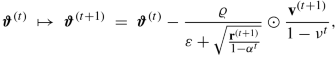
nadam is the Nesterov-accelerated [284] version of adam. Similarly as when going from (7.19)–(7.20) to (7.23), the acceleration is obtained by a shift of 1 in the velocity parameter, thus, consider the Nesterov-accelerated adam update


7.2.3.5 Maximum Likelihood Estimation and Over-fitting
As explained above, we model the mean of the datum (Y, x) by a deep FN network
for a network parameter \(\boldsymbol {\vartheta } \in {\mathbb R}^r\). MLE of this network parameter requires solving for given data Y

In Fig. 7.5 we give a schematic figure of a loss surface \(\boldsymbol {\vartheta } \mapsto {\mathfrak D}(\boldsymbol {Y}, \boldsymbol {\vartheta })\) for a (low-dimensional) example \(\boldsymbol {\vartheta } \in {\mathbb R}^2\). The two plots show the same loss surface from two different angles. This loss surface has three (local) minimums (red color), and the smallest one (global minimum) gives the MLE \(\widehat {\boldsymbol {\vartheta }}^{\text{MLE}}\).

Schematic figure of in-sample over-fitting (red), under-fitting (blue) and extracting systematic effects (green)
In general, this global minimum cannot be found for more complex network architectures because the loss surface typically has a complicated structure for high-dimensional parameter spaces. Is this a problem in FN network fitting? Not really! We are going to explain why. The universality theorems in Sect. 7.2.2 state that more complex FN networks have an excellent approximation capacity. If we translate this to our statistical modeling problem it means that the observations Y can be approximated arbitrarily well by sufficiently complex FN networks. In particular, for a given complex network architecture, the MLE \(\widehat {\boldsymbol {\vartheta }}^{\text{MLE}}\) will provide the optimal fit of this architecture to the data Y , and, as a result, this network does not only reflect the systematic effects in the data but also the noisy part. This behavior is called (in-sample) over-fitting to the learning data \(\mathcal {L}\). It implies that such statistical models typically have a poor generalization to unseen (out-of-sample) test data \(\mathcal {T}\); this is illustrated by the red color in Fig. 7.6. For this reason, in general, we are not interested in finding the MLE \(\widehat {\boldsymbol {\vartheta }}^{\text{MLE}}\) of 𝜗 in FN network regression modeling, but we would like to find a parameter estimate \(\widehat {\boldsymbol {\vartheta }}\) that (only) extracts the systematic effects from the learning data \(\mathcal {L}\). This is illustrated by the different colors in Figs. 7.5 and 7.6, where we assume: (a) red color provides models with a poor generalization power due to over-fitting, (b) blue color provides models with a poor generalization power, too, because these parametrizations do not explain the systematic effects in the data at all (called under-fitting), and (c) green color gives good parametrizations that explain the systematic effects in the data and generalize well to unseen data. Thus, the aim is to find parametrizations that are in the green area of Fig. 7.5. This green area emphasizes that we lose the notion of uniqueness because there are infinitely many models in the green area that have a comparable generalization power. Next we explain how we can exploit the gradient descent algorithm to make it useful for finding parametrizations in the green area. Remark 7.8. The loss surface considerations in Fig. 7.5 are based on a fixed network architecture. Recent research promotes the so-called Graph HyperNetwork (GHN) that is a (hyper-)network which tries to find the optimal network architecture and its parametrization by an additional network, we refer to Zhang et al. [402] and Knyazev et al. [219].

Partition of entire data \(\mathcal {D}\) (lhs) into learning data \(\mathcal {L}\) and test data \(\mathcal {T}\) (middle), and into training data \(\mathcal {U}\), validation data \(\mathcal {V}\) and test data \(\mathcal {T}\) (rhs)
7.2.3.6 Regularization Through Early Stopping
As stated above, if we run the gradient descent algorithm with properly tempered learning rates it will converge to a local minimum of the loss function, which means that the resulting FN network over-fits to the learning data. For this reason we need to early stop the gradient descent algorithm beforehand. Coming back to Fig. 7.5, typically, we start the gradient descent algorithm somewhere in the blue area of the loss surface (supposed that the red area is a sparse set on the loss surface). Visually speaking, the gradient descent algorithm then walks down the valley (green, yellow and red area) by exploiting locally optimal steps. Since at the early stage of the algorithm the systematic effects play a dominant role over the noisy part, the gradient descent algorithm learns these systematic effects at this first stage (blue area in Fig. 7.5). When the algorithm arrives at the green area the noisy part in the data starts to increasingly influence the model calibration (gradient descent steps), and, henceforth, at this stage the algorithm should be stopped, and the learned parameter should be selected for predictive modeling. This early stopping is an implicit way of regularization, because it implies that we stop the parameter fitting before the parameters start to learn very individual features of the (noisy) data (and take extreme values).
This early stopping point is determined by doing an out-of-sample analysis. This requires the learning data \(\mathcal {L}\) to be further split into training data \(\mathcal {U}\) and validation data \(\mathcal {V}\). The training data \(\mathcal {U}\) is used for gradient descent parameter learning, and the validation data \(\mathcal {V}\) is used for tracking the over-fitting by an instantaneous (out-of-sample) validation analysis. This partition is illustrated in Fig. 7.7, which also highlights that the validation data \(\mathcal {V}\) is disjoint from the test data \(\mathcal {T}\), the latter only being used in the final step for comparing different statistical models (e.g., a GLM vs. a FN network). That is, model comparison is done in a proper out-of-sample manner on \(\mathcal {T}\), and each of these models is only fit on \(\mathcal {U}\) and \(\mathcal {V}\). Thus, for FN network fitting with early stopping we need a reasonable amount of data that can be split into 3 sufficiently large data sets so that each is suitable for its purpose.

Training loss \({\mathfrak D}(\mathcal {U}, \boldsymbol {\vartheta }^{(t)})\) vs. validation loss \({\mathfrak D}(\mathcal {V}, \boldsymbol {\vartheta }^{(t)})\) over different iterations t ≥ 0 of the SGD algorithm
For early stopping we partition the learning data \(\mathcal {L}\) into training data \(\mathcal {U}\) and validation data \(\mathcal {V}\). The plain vanilla gradient descent algorithm can then be changed as follows.
________________________________________________________________________________________________
Plain vanilla gradient descent algorithm with early stopping
________________________________________________________________________________________________
-
1.
Choose an initial network parameter \(\boldsymbol {\vartheta }^{(0)} \in {\mathbb R}^r\).
-
2.
Iterate for t ≥ 0 until the early stopping criterion is met:
-
(a)
Calculate the gradient \(\nabla _{\boldsymbol {\vartheta }}{\mathfrak D}(\mathcal {U}, \boldsymbol {\vartheta })\) in network parameter 𝜗 = 𝜗 (t) on the training data \(\mathcal {U}\) using (7.16) and the back-propagation method of Proposition 7.5 (for the hyperbolic tangent activation function).
-
(b)
Make the gradient descent step for a suitable learning rate ϱ t+1 > 0
$$\displaystyle \begin{aligned} \boldsymbol{\vartheta}^{(t)} ~\mapsto ~\boldsymbol{\vartheta}^{(t+1)} =\boldsymbol{\vartheta}^{(t)}-\varrho_{t+1} \nabla_{\boldsymbol{\vartheta}}{\mathfrak D}(\mathcal{U}, \boldsymbol{\vartheta}^{(t)}). \end{aligned}$$ -
(c)
Calculate the validation loss \({\mathfrak D}(\mathcal {V}, \boldsymbol {\vartheta }^{(t)})\) on the validation data \(\mathcal {V}\).
-
(d)
Stop the algorithm if the validation loss increases, i.e., if
$$\displaystyle \begin{aligned} {\mathfrak D}(\mathcal{V}, \boldsymbol{\vartheta}^{(t)})~>~{\mathfrak D}(\mathcal{V}, \boldsymbol{\vartheta}^{(t-1)}),{} \end{aligned} $$(7.27)and return the learned parameter (estimate) \(\widehat {\boldsymbol {\vartheta }}=\boldsymbol {\vartheta }^{(t-1)}\).
-
(a)
__________________________________________________________________
In applications we use the SGD algorithm that can also have erratic steps because not all random (mini-)batches are necessarily typical representations of the data. In such cases we should use more sophisticated stopping criteria than (7.27), for instance, early stop if the validation loss increases five times in a row.
Figure 7.8 provides an example of the application of the SGD algorithm on training data \(\mathcal {U}\) and validation data \(\mathcal {V}\). The training loss is in blue color and the validation loss in green color. We observe that the validation loss has its minimum after 52 epochs (orange vertical line), and hence the fitting algorithm should be stopped at this point. We give a couple of remarks concerning Fig. 7.8:
-
The learning data \(\mathcal {L}\) exactly corresponds to the claims frequency data of Sect. 5.2.4, see also Table 5.2. We take 10% as validation data which gives \(|\mathcal {U}|=549'185\) and \(|\mathcal {V}|=61'021\). For the SGD algorithm we use batches of size 10′000 which implies that one epoch corresponds to ⌊549′185∕10′000⌋ = 54 gradient descent steps. For batches of size 10′000 we expect an approximate estimation precision on an average frequency of \(\bar {\lambda }=7.36\%\) in the Poisson model of
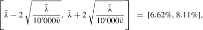
Fig. 7.9 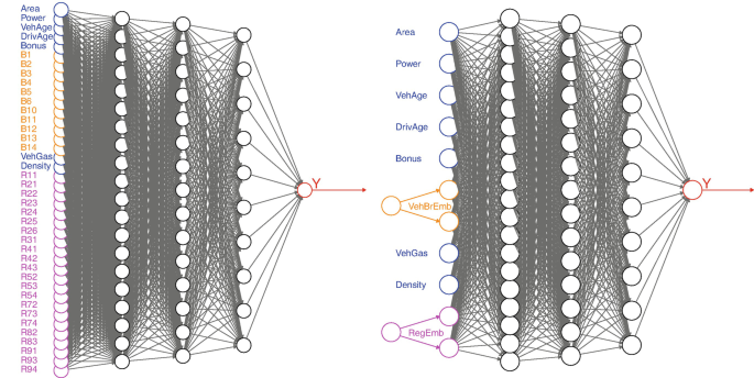
(lhs) One-hot encoding with q 0 = 40, and (rhs) embedding layers for VehBrand and Region with embedding dimension b = 2 and q 0 = 11; the remaining network architecture is identical with (q 1, q 2, q 3) = (20, 15, 10) for depth d = 3
with an average exposure \(\bar {v}=0.5283\) on our learning data, we also refer to Example 3.22.
-
The FN network architecture used in Fig. 7.8 is the one shown in Fig. 7.2 using one-hot encoding for categorical variables, see Sect. 7.3.1, below, and the responses are modeled by a Poisson distribution.
-
The training loss \({\mathfrak D}(\mathcal {U}, \boldsymbol {\vartheta }^{(t)})\), blue curve in Fig. 7.8, is a bit wiggly which comes from the fact that we use a SGD where not every batch leads to the optimal decrease in loss. Remark that the loss figures in the graph correspond to average losses over an entire epoch, i.e., in our case an average over 54 SGD steps. Also remark that the y-scale does not show the Poisson deviance loss: we use the loss figures provided by keras [77] and these figures drop all terms of the deviance loss that are not relevant for parameter estimation.


We close this section with remarks.
Remarks 7.9.
-
We perform early stopping because otherwise a complex FN network would in-sample over-fit to the learning data. At this stage, one could be tempted to choose a smaller network to prevent from over-fitting. In general, this is not a sensible thing to do because the network needs sufficient flexibility to be able to be fitted to the data. That is, we need some redundancy in the model to be able to successfully apply the SGD algorithm, otherwise the algorithm may get trapped in saddlepoints or bottlenecks. Thus, the chosen network architecture should be above the bound of a necessary minimal complexity, and different architectures above this bound will provide similar accuracy (without a clear winner).
-
The chosen network will contain certain elements of randomness, and different runs of the SGD algorithm will provide different solutions. Firstly, the initialization \(\boldsymbol {\vartheta }^{(0)} \in {\mathbb R}^r\) of the algorithm is chosen at random, and since we early stop the algorithm and because we do not have a unique optimal point, the chosen solution will depend on this random initialization. Secondly, the split between training and validation data is done at random, and thirdly the partitioning of the training data into mini-batches is done at random. All these random elements make the early stopped SGD solution non-unique.
-
Early stopping implies that the chosen network parameter estimate \(\widehat {\boldsymbol {\vartheta }}\) does not correspond to a solution of the score equations and, henceforth, asymptotic results about MLEs do not apply, see Theorem 3.28.
7.3 Feed-Forward Neural Network Examples
7.3.1 Feature Pre-processing
Similarly to GLMs, we also need to pre-process the feature components in FN network regression modeling. The former Sect. 5.2.2 for GLMs has been called ‘feature engineering’ because we need to bring the feature components into an appropriate functional form w.r.t. the given regression task. The present section is called ‘feature pre-processing’ because we do not need to engineer the features for FN networks. We only need to bring them into a suitable (tabular) form to enter the network, and the network will then do an automated feature engineering through representation learning.
7.3.1.1 Categorical Feature Components: One-Hot Encoding
The categorical features have been treated by dummy coding within GLMs. Dummy coding provides full rank design matrices. For FN network regression modeling the full rank property is not important because, anyway, we neither have a single (local) minimum in the objective function, nor do we want to calculate the MLE of the network parameter. Typically, in FN network regression modeling one uses one-hot encoding for the categorical variables that encodes every level by a unit vector. Assume the raw feature component \(\widetilde {x}_j\) is a categorical variable taking K different levels {a 1, …, a K}. One-hot encoding is obtained by the embedding map

An explicit example is given in Table 7.2 which should be compared to Table 5.1.
 as row vectors
7.3.1.2 Continuous Feature Components
The continuous feature components do not need any pre-processing but they can directly enter the FN network which will take care of representation learning. However, an efficient use of gradient descent methods typically requires that all feature components live on a similar scale and that they are roughly uniformly spread across their domains. This makes gradient descent steps more efficient in exploiting the relevant directions.
One possibility is to use the MinMaxScaler. Let \(x_j^-\) and \(x_j^+\) be the minimal and maximal possible feature values of the continuous feature component x j, i.e., \(x_j \in [x_j^-,x_j^+]\). We transform this continuous feature component to unit scale for all data 1 ≤ i ≤ n by
The resulting feature values \((x_{i,j}^{\text{MM}})_{1\le i \le n}\) should roughly be uniformly spread across the interval [−1, 1]. If this is not the case, for instance, because we have outliers in the feature values, we may first transform them non-linearly to get more uniformly spread values. For example, we consider the Density of the car frequency example on the log scale.
An alternative to the MinMaxScaler is to consider normalization with the empirical mean \(\bar {x}_j\) and the empirical standard deviation \(\hat {\sigma }_j\) over all data x i,j. That is,
It depends on the application whether the MinMaxScaler or normalization with the empirical mean and standard deviation works better. Important in applications is that we use exactly the same values for the normalization of training data \(\mathcal {U}\), validation data \(\mathcal {V}\) and test data \(\mathcal {T}\), to make the same network applicable to all these data sets. For notational convenience we will drop the upper index in \(x_{i,j}^{\text{MM}}\) or \(x_{i,j}^{\text{sd}}\), respectively, and we throughout assume that all feature components are appropriately pre-processed.
7.3.2 Lab: Poisson FN Network for Car Insurance Frequencies
We present a first FN network example applied to the French MTPL claim frequency data studied in Sect. 5.2.4. We assume that the claim counts N i are independent and Poisson distributed with claim count density (5.26), where we replace the GLM regression function \(\boldsymbol {x} \mapsto \exp \langle \boldsymbol {\beta }, \boldsymbol {x} \rangle \) by a FN network regression function
We use a FN network of depth d = 3 having number of neurons (q 1, q 2, q 3) = (20, 15, 10) and using the hyperbolic tangent activation function. We pre-process the categorical variables VehBrand and Region by one-hot encoding providing input dimensions 11 and 22, respectively. The binary variable VehGas is encoded as 0–1. Because of scarcity of data we right-censor the continuous variables VehAge at 20, DrivAge at 90 and BonusMalus at 150, and we transform Density to the log scale. We then apply to each of these (modified) continuous variables Area, VehPower, VehAge, DrivAge, BonusMalus and log(Density) a MinMaxScaler. This provides us with an input dimension q 0 = 11 + 22 + 1 + 6 = 40. The resulting FN network is illustrated in Fig. 7.2, with the one-hot encoded variables VehBrand in orange color and Region in magenta color. It has a network parameter \(\boldsymbol {\vartheta } \in {\mathbb R}^r\) of dimension r = 1′306.
Listing 7.1 FN network of depth d = 3 using the R library keras [77]

Listing 7.2 FN network illustrated in Fig. 7.2

Listing 7.3 Fitting a FN network using the R library keras [77]

This network is implemented in R using the library keras [77]. The code is provided in Listing 7.1 and the resulting network architecture is summarized in Listing 7.2. This network is now fitted to the data. We use a batch size of 10’000, we use the nadam version of SGD, we use 10% of the learning data \(\mathcal {L}\) as validation data \(\mathcal {V}\) and the remaining 90% as training data \(\mathcal {U}\). We then run the corresponding SGD algorithm and we retrieve the network with the lowest validation loss using a callback. This is illustrated in Listing 7.3. The fitting performance on the training and validation data is illustrated in Fig. 7.8, and we retrieve the network calibration after the 52th epoch because it has the lowest validation loss. The results are presented in Table 7.3.
From the results of Table 7.3 we conclude that the FN network outperforms model Poisson GLM3 (out-of-sample) since it has a (clearly) lower out-of-sample deviance loss on the test data \(\mathcal {T}\). This may indicate that there is an interaction between the feature components that has not been captured in the GLM. The run time of 51s corresponds to the run time until the minimal validation loss is reached, of course, in practice we need to continue beyond this minimal validation loss to ensure that we have really found the minimum. Finally, and importantly, we observe that this early stopped FN network calibration does not meet the balance property because the resulting average frequency of this fitted model of 6.96% is below the empirical frequency of 7.36%. This is a major deficiency of this FN network fitting approach, and this is going to be discussed further in Sect. 7.4.2, below.
We can perform a detailed analysis about different batch sizes, variants of SGD methods, run times, etc. We briefly summarize our findings; this summary is also based on the findings in Ferrario et al. [127]. We have fitted this model on batches of sizes 2’000, 5’000, 10’000 and 20’000, and it seems that a batch size around 5’000 has the best performance, both concerning out-of-sample performance and run time to reach the minimal validation loss. Comparing the different optimizers rmsprop, adam and nadam, a clear preference can be given to nadam: the resulting prediction accuracy is similar in all three optimizers (they all reach the green area in Fig. 7.5), but nadam reaches this optimal point in half of the time compared to rmsprop and adam.
We conclude by highlighting that different initial points 𝜗 (0) of the SGD algorithm will give different network calibrations, and differences can be considerable. This is discussed in Sect. 7.4.4, below. Moreover, we could explore different network architectures, more simple ones, more complex ones, different activation functions, etc. The results of these different architectures will not be essentially different from our results, as long as the networks are above a minimal complexity bound. This closes our first example on FN networks and this example is the benchmark for refined versions that are presented in the subsequent sections.
7.4 Special Features in Networks
7.4.1 Special Purpose Layers
So far, our networks consist of stacked FN layers, and information is passed in a directed acyclic feed-forward path from one to the next FN layer. In this section we discuss special purpose layers that perform a specific task in a FN network. These include embedding layers, drop-out layers and normalization layers. These modules should be seen as add-ons to the FN layers. Besides these add-ons, there are also recurrent layers and convolutional layers. These two types of layers are going to be discussed in own chapters, below, because their importance goes beyond just being add-ons to the FN layers.
7.4.1.1 Embedding Layers for Categorical Feature Components
The categorical feature components have been treated either by dummy coding or by one-hot encoding, and this has resulted in numerous network parameters in the first FN layer, see Fig. 7.2. Natural language processing (NLP) treats categorical feature components differently, namely, it embeds categorical feature components (or words in NLP) into a Euclidean space \({\mathbb R}^b\) of a small dimension b. This small dimension b is a hyper-parameter that has to be selected by the modeler, and which, typically, is selected much smaller than the total number of levels of the categorical feature. This embedding technique is quite common in NLP, see Bengio et al. [27,28,29], but it goes beyond NLP applications, see Guo–Berkhahn [176], and it has been introduced to the actuarial community by Richman [312, 313] and the tutorial of Schelldorfer–Wüthrich [329].
We assume the same set-up as in dummy coding (5.21) and in one-hot encoding (7.28), namely, that we have a raw categorical feature component \(\widetilde {x}_j\) taking K different levels {a 1, …, a K}. In one-hot encoding these K levels are mapped to the K unit vectors of the Euclidean space \({\mathbb R}^K\), and consequently all levels have the same mutual Euclidean distance. This does not seem to be the best way of comparing the different levels because in our regression analysis we would like to identify the levels that are more similar w.r.t. the regression task and, thus, these should cluster. For an embedding layer one chooses a Euclidean space \({\mathbb R}^b\) of a dimension b < K, typically being (much) smaller than K. One then considers the embedding map

That is, every level a k receives a vector representation \(\boldsymbol {e}^{(k)} \in {\mathbb R}^b\) which is lower dimensional than its one-hot encoding counterpart in \({\mathbb R}^K\). Proximity of the representations e (k) and \(\boldsymbol {e}^{(k')}\) in \({\mathbb R}^b\), i.e., of two levels a k and \(a_{k'}\), should be related to similarity w.r.t. the regression task at hand. Such an embedding involves K vectors \(\boldsymbol {e}^{(k)}\in {\mathbb R}^b\) of dimension b, thus, it involves Kb parameters, called embedding weights.
In network modeling, these embedding weights e (1), …, e (K) can also be learned during gradient descent training. Basically, it just means that for the categorical variables we add an additional embedding layer before the first FN layer z (1), i.e., we increase the depth of the network by 1 for the categorical feature components (by a layer that is not fully connected). This is illustrated in Fig. 7.9 (rhs) for the French MTPL insurance example of Sect. 7.3.2. The graph on the left-hand side shows the network if we apply one-hot encoding to the categorical variables VehBrand and Region; this results in a network parameter of dimension r = 1′306. The graph on the right-hand side first embeds VehBrand and Region into two 2-dimensional spaces, illustrated by the orange and magenta circles. These embeddings are concatenated with the remaining feature components, which then provides a new dimension q 0 = 7 + 2 + 2 = 11 in that example. This results in a network parameter of dimension r = 726 + 22 + 44 = 792, where 22 + 44 = 66 stands for the 2-dimensional embedding weights of the 11 VehBrands and the 22 French Regions, see Listing 7.5. Example 7.10 (Embedding Layers for Categorical Features). We revisit the example of Sect. 7.3.2, but we replace one-hot encoding of the categorical variables by embedding layers of dimension b = 2. The corresponding R code is given in Listing 7.4 and the resulting model is illustrated in Listing 7.5 and Fig. 7.9 (rhs).
Listing 7.4 FN network of depth d = 3 using embedding layers

Listing 7.5 Summary of FN network of Fig. 7.9 (rhs) using embedding layers of dimension b = 2

Apart from replacing one-hot encoding by embedding layers, we use exactly the same FN network architecture as in Sect. 7.3.2 and we apply the same fitting strategy in terms of batch sizes, optimizer and early stopping strategy. The results are presented in Table 7.4.
A first remark is that the model calibration takes longer using embedding layers compared to one-hot encoding. The main reason for this is that having an embedding layer increases the depth of the network by one layer, as can be seen from Fig. 7.9. Therefore, the back-propagation takes more time, and the convergence is slower requiring more gradient descent steps. We have less over-fitting as can be seen from Fig. 7.10. The final fitted model has a slightly better out-of-sample performance compared to the one-hot encoding one. However, this slight improvement in the performance should not be overstated because, as explained in Remarks 7.9, there are a couple of elements of randomness involved in SGD fitting, and choosing a different seed may change the results. We remark that the balance property is not fulfilled because the average frequency of the fitted model does not meet the empirical frequency, see the last column of Table 7.4; we come back to this in Sect. 7.4.2, below.

Training loss \({\mathfrak D}(\mathcal {U}, \boldsymbol {\vartheta }^{(t)})\) vs. validation loss \({\mathfrak D}(\mathcal {V}, \boldsymbol {\vartheta }^{(t)})\) over different iterations t ≥ 0 of the SGD algorithm in the deep FN network with embedding layers for categorical variables
A major advantage of using embedding layers for the categorical variables is that we receive a continuous representation of nominal variables, where proximity can be interpreted as similarity for the regression task at hand. This is nicely illustrated in Fig. 7.11 which shows the resulting 2-dimensional embeddings \(\boldsymbol {e}^{\mathtt {VehBrand}}\in {\mathbb R}^2 \) and \(\boldsymbol {e}^{\mathtt {Region}} \in {\mathbb R}^2\) of the categorical variables VehBrand and Region. The Region embedding \(\boldsymbol {e}^{\mathtt {Region}} \in {\mathbb R}^2\) shows surprising similarities with the French map, for instance, Paris region R11 is adjacent to R23, R22, R21, R26, R24 (which is also the case in the French map), the Isle of Corsica R94 and the South of France R93, R91 and R73 are well separated from other regions, etc. Similar observations can be made for the embedding of VehBrand, Japanese cars B12 are far apart from the other cars, cars B1, B2, B3 and B6 (Renault, Nissan, Citroen, Volkswagen, Audi, Skoda, Seat and Fiat) cluster, etc. \(\blacksquare \)

Embedding weights \(\boldsymbol {e}^{\mathtt {VehBrand}}\in {\mathbb R}^2\) and \(\boldsymbol {e}^{\mathtt {Region}}\in {\mathbb R}^2\) of the categorical variables VehBrand and Region for embedding dimension b = 2
7.4.1.2 Drop-Out Layers and Regularization
Above, over-fitting to the learning data has been taken care of by early stopping. In view of Sect. 6.2 one could also use regularization. This can easily be obtained by replacing (7.14), for instance, by the following L p-regularized counterpart
for some p ≥ 1, regularization parameter λ > 0 and where the reduced network parameter \(\boldsymbol {\vartheta }_-\in {\mathbb R}^{r-1}\) excludes the intercept parameter β 0 of the output layer, we also refer to (6.4) in the context of GLMs. For grouped penalty terms we refer to (6.21). The difficulty with this approach is the tuning of the regularization parameter(s) λ: run time is one issue, suitable grouping is another issue, and non-uniqueness of the optimal network a further one that can substantially distort the selection of reasonable regularization parameters.
A more popular method to prevent from over-fitting individual neurons in a FN layer to a certain task are so-called drop-out layers. A drop-out layer is an additional layer between FN layers that removes at random during gradient descent training neurons from the network, i.e., in each gradient descent step, any of the earmarked neurons is offset independently from the others with a fixed probability δ ∈ (0, 1). This random removal will imply that the composite of the remaining neurons needs to be sufficiently well balanced to take over the role of the dropped-out neurons. Therefore, a single neuron cannot be over-trained to a certain task because it needs to be able play several different roles. Drop-out has been introduced by Srivastava et al. [345] and Wager et al. [373].
Listing 7.6 FN network of depth d = 3 using a drop-out layer, ridge regularization and a normalization layer

Listing 7.6 gives an example, where we add a drop-out layer with a drop-out probability of δ = 0.01 after the first FN layer, and in the second FN layer we apply ridge regularization to the weights \((w^{(2)}_{1,1}, \ldots , w^{(2)}_{q_1,q_2})\), i.e., excluding the intercepts \(w^{(2)}_{0,j}\), 1 ≤ j ≤ q 2. Both the drop-out layer and regularization are only used during the gradient descent fitting, and these network features are disabled during the prediction.
Drop-out is closely related to ridge regularization as the following linear Gaussian regression example shows; this consideration is taken from Section 18.6 of Efron–Hastie [117]. Assume we have a linear regression problem with square loss function
We assume in this Gaussian case that the observations and the features are standardized, see Sect. 6.2.4. This means that \(\sum _{i=1}^n Y_i=0\), \(\sum _{i=1}^n x_{i,j}=0\) and \(n^{-1}\sum _{i=1}^n x^2_{i,j}=1\), for all 1 ≤ j ≤ q. This standardization implies that we can omit the intercept parameter β 0 because its MLE is equal to 0.
We introduce i.i.d. drop-out random variables I i,j for 1 ≤ i ≤ n and 1 ≤ j ≤ q with (1 − δ)I i,j being Bernoulli distributed with probability 1 − δ ∈ (0, 1). This scaling implies \({\mathbb E}[I_{i,j}]=1\). Using these Bernoulli random variables we modify the above square loss function to
i.e., every individual component x i,j can drop out independently of the others. Gaussian MLE requires to set the gradient of \({\mathfrak D}_I(\boldsymbol {Y}, \boldsymbol {\beta })\) w.r.t. \(\boldsymbol {\beta } \in {\mathbb R}^{q}\) equal to zero. The average score equation is given by (we average over the drop-out random variables I i,j)

where we have used the normalization of the columns of the design matrix \(\mathfrak {X} \in {\mathbb R}^{n\times {q}}\) (we drop the intercept column). This is ridge regression in the linear Gaussian case with a regularization parameter λ = δ∕(2(1 − δ)) > 0 for δ ∈ (0, 1), see (6.9).
7.4.1.3 Normalization Layers
In (7.29) and (7.30) we have discussed that the continuous feature components should be pre-processed so that all components live on the same scale, otherwise the gradient descent fitting may not be efficient. A similar phenomenon may occur with the learned representations z (m:1)(x i) in the FN layers 1 ≤ m ≤ d. In particular, this is the case if we choose an unbounded activation function ϕ. For this reason, it can be advantageous to rescale the components \(z_j^{(m:1)}(\boldsymbol {x}_i)\), 1 ≤ j ≤ q m, in a given FN layer back to the same scale. To achieve this, a normalization step (7.30) is applied to every neuron \(z_j^{(m:1)}(\boldsymbol {x}_i)\) over the given cases i in the considered (mini-)batch. This involves two more parameters (for the empirical mean and the empirical standard deviation) in each neuron of the corresponding FN layer. Note, however, that all these operations are of a linear nature. Therefore, they do not affect the predictive model (i.e., these operations cancel in the scalar products in (7.6)), but they may improve the performance of the gradient descent algorithm.
The code in Listing 7.6 uses a normalization layer on line 6. In our applications, it has not been necessary to use these normalization layers, as it has not led to better run times in SGD algorithms; note that our networks are not very deep and they use the symmetric and bounded hyperbolic tangent activation function.
7.4.2 The Balance Property in Neural Networks
We have seen in Table 7.4 that our FN network outperforms the GLM for claim frequency prediction in terms of a lower out-of-sample loss. We interpret this as follows. Feature engineering has not been done in the most optimal way for the GLM because the FN network finds modeling structure that is not present in the selected GLM. As a consequence, the FN network provides a better generalization to unseen data, i.e., we can better predict new data on a granular level with the FN network. However, having a more precise model on an individual policy level does not necessarily imply that the model also performs better on a global portfolio level. In our example we see that we may have smaller errors on an individual policy level, but these smaller errors do not aggregate to a more precise model in the average portfolio frequency. In our case, we have a misspecification of the average portfolio frequency, see the last column of Table 7.4. This is a major deficiency in insurance pricing because it may result in a misspecification of the overall price level, and this requires a correction. We call this correction bias regularization.
7.4.2.1 Simple Bias Regularization
The straightforward correction is to adjust the intercept parameter \(\beta _0 \in {\mathbb R}\) accordingly. That is, compare the empirical mean
to the model average of the fitted FN network
where  is the learned network parameter from the (early stopped) SGD algorithm. The output of this fitted model reads as
where the hat in \( \widehat {\boldsymbol {z}}^{(d:1)}\) indicates that we use the estimated weights \(\widehat {\boldsymbol {w}}^{(m)}_l\), 1 ≤ l ≤ q m, 1 ≤ m ≤ d, in the FN layers. The balance property can be rectified by replacing \(\widehat {\beta }_0\) by the solution \(\widehat {\widehat {\beta }}_0\) of the following identity

Since g −1 is continuous and strictly monotone, there is a unique solution to this requirement supposed that the range of g −1 covers the support of the Y i’s. If we work with the log-link g(⋅) = log(⋅), this can easily be solved and we obtain
7.4.2.2 Sophisticated Bias Regularization Under the Canonical Link Choice
If we work with the canonical link g = h = (κ′)−1, we can do better because the MLE of such a GLM automatically provides the balance property, see Corollary 5.7. Choose the SGD learned network parameter  . Denote by \( \widehat {\boldsymbol {z}}^{(d:1)}\) the fitted network architecture that is based on the estimated weights \(\widehat {\boldsymbol {w}}^{(1)}_1, \ldots , \widehat {\boldsymbol {w}}^{(d)}_{q_d}\). This allows us to study the learned representations of the raw features x
1, …, x
n in the last FN layer. We denote these learned representations by
. Denote by \( \widehat {\boldsymbol {z}}^{(d:1)}\) the fitted network architecture that is based on the estimated weights \(\widehat {\boldsymbol {w}}^{(1)}_1, \ldots , \widehat {\boldsymbol {w}}^{(d)}_{q_d}\). This allows us to study the learned representations of the raw features x
1, …, x
n in the last FN layer. We denote these learned representations by
These learned representations can be used as new features to explain the response Y . We define the feature engineered design matrix by

Based on this new design matrix \(\widehat {\mathfrak {X}}\) we can run a classical GLM receiving a unique MLE \(\widehat {\boldsymbol {\beta }}^{\text{MLE}} \in {\mathbb R}^{q_d+1}\) supposed that this design matrix has a full rank q d + 1 ≤ n, see Proposition 5.1. Since we work with the canonical link, this re-calibrated FN network will automatically satisfy the balance property, and the resulting regression function reads as
This is the proposal of Wüthrich [390]. We give some remarks.
Remarks 7.11.
-
This additional MLE step for the output parameter \(\boldsymbol {\beta } \in {\mathbb R}^{q_d+1}\) may lead to over-fitting. In that case one might choose a lower dimensional last FN layer. Alternatively, one might explore a more early stopping rule in SGD.
-
Wüthrich [390] also explores other bias correction methods like regularization using shrinkage. In combination with regression trees one can achieve averages on pre-defined sub-portfolios. We will not further explore these other approaches because they are less robust and more difficult in the applications.
Example 7.12 (Balance Property in Networks). We apply this additional MLE step to the two FN networks of Table 7.4. Note that in these two examples we consider a Poisson model using the canonical link for g, thus, the resulting adjusted network (7.33) will automatically satisfy the balance property, see Corollary 5.7.
Listing 7.7 Balance property adjustment (7.33)

In Listing 7.7 we illustrate the necessary code that has to be added to Listings 7.1–7.3. On lines 7–8 of Listing 7.7 we retrieve the learned representations (7.32) which are used as the new features in the Poisson GLM on lines 13–14. The resulting MLE \(\widehat {\boldsymbol {\beta }}^{\text{MLE}} \in {\mathbb R}^{q_d+1}\) is imputed to the network parameter \(\widehat {\boldsymbol {\vartheta }}\) on lines 17–20. Table 7.5 shows the performance of the resulting bias regularized FN networks.
Firstly, we observe from the last column of Table 7.5 that, indeed, the bias regularization step (7.33) provides the balance property. In general, in-sample losses (have to) decrease because \(\widehat {\boldsymbol {\beta }}^{\text{MLE}}\) is (in-sample) more optimal than the early stopped SGD solution \(\widehat {\boldsymbol {\beta }}\). Out-of-sample this leads to a small improvement in the one-hot encoded variant and a small worsening in the embedding variant, i.e., the latter slightly over-fits in this additional MLE step. However, these differences are comparably small so that we do not further worry about the over-fitting, here. This closes this example. \(\blacksquare \)
7.4.2.3 Auto-Calibration for Bias Regularization
We present another approach of correcting for the potential failure of the balance property. This method does not depend on a particular type of regression model, i.e., it can be applied to any regression model. This proposal goes back to Denuit et al. [97], and it is based on the notion of auto-calibration introduced by Patton [297] and Krüger–Ziegel [227]. We first describe auto-calibration and its implications. Definition 7.13. The random variable Z is an auto-calibrated forecast of random variable Y if \({\mathbb E}[Y|Z]=Z\), a.s.
If the response Y is described by the features X = x, we consider the conditional mean of Y , given X,
This conditional mean μ(X) is an auto-calibrated forecast for the response Y . Use the tower property and note that σ(μ(X)) ⊂ σ(X) to receive, a.s.,
For the further understanding of auto-calibration and forecast dominance, we introduce the concept of convex order; forecast dominance has been introduced in Definition 4.20. Definition 7.14 (Convex Order). A random variable Z 1 is bigger in convex order than a random variable Z 2, write Z 1 ≽cx Z 2, if \({\mathbb E}[\Psi (Z_1)] \ge {\mathbb E}[\Psi (Z_2)]\), for all convex functions Ψ for which the expectations exist.
By Strassen’s theorem [346], Z
1 ≽cx
Z
2 if and only if there exist random variables \(Z_1^{\prime }\) and \(Z_2^{\prime }\) with  and
and  and \({\mathbb E}[Z_1^{\prime }|Z_2^{\prime }]=Z_2^{\prime }\), a.s. In particular, the convex order Z
1 ≽cx
Z
2 implies that Var(Z
1) ≥Var(Z
2) and \({\mathbb E}[Z_1]={\mathbb E}[Z_2]\). The latter follows from Strassen’s theorem and the tower property, and the former follows from the latter and the convex order by using the explicit choice Ψ(x) = x
2. Thus, the random variable Z
1 is more volatile than Z
2, both having the same mean. The following theorem shows that this additional volatility is a favorable property in terms of forecast dominance under auto-calibration. Theorem 7.15 (Krüger–Ziegel [227, Theorem 3.1], Without Proof). Assume that \(\widehat {\mu }_1\) and \(\widehat {\mu }_2\) are auto-calibrated forecasts for the random variable Y . Predictor \(\widehat {\mu }_1\) forecast dominates \(\widehat {\mu }_2\) if and only if \(\widehat {\mu }_1 \succeq _{\text{cx}} \widehat {\mu }_2\).
and \({\mathbb E}[Z_1^{\prime }|Z_2^{\prime }]=Z_2^{\prime }\), a.s. In particular, the convex order Z
1 ≽cx
Z
2 implies that Var(Z
1) ≥Var(Z
2) and \({\mathbb E}[Z_1]={\mathbb E}[Z_2]\). The latter follows from Strassen’s theorem and the tower property, and the former follows from the latter and the convex order by using the explicit choice Ψ(x) = x
2. Thus, the random variable Z
1 is more volatile than Z
2, both having the same mean. The following theorem shows that this additional volatility is a favorable property in terms of forecast dominance under auto-calibration. Theorem 7.15 (Krüger–Ziegel [227, Theorem 3.1], Without Proof). Assume that \(\widehat {\mu }_1\) and \(\widehat {\mu }_2\) are auto-calibrated forecasts for the random variable Y . Predictor \(\widehat {\mu }_1\) forecast dominates \(\widehat {\mu }_2\) if and only if \(\widehat {\mu }_1 \succeq _{\text{cx}} \widehat {\mu }_2\).
Recall that forecast dominance of \(\widehat {\mu }_1\) over \(\widehat {\mu }_2\) was defined as follows, see Definition 4.20,
for all Bregman divergences D ψ. Strassen’s theorem tells us that \(\widehat {\mu }_1\) is more volatile than \(\widehat {\mu }_2\) (both being auto-calibrated and unbiased for \({\mathbb E}[Y]\)) and this additional volatility implies that the former auto-calibrated predictor can better follow Y . This provides the superior forecast dominance of \(\widehat {\mu }_1\) over \(\widehat {\mu }_2\). This relation is most easily understood by the following example. Consider (Y, X) as above. Assume that the feature \(\widetilde {\boldsymbol {X}}\) is a sub-variable of the feature X by dropping some of the components of X. Naturally, we have \(\sigma (\widetilde {\boldsymbol {X}})\subset \sigma (\boldsymbol {X})\), and both sets of information provide auto-calibrated forecasts
The tower property and Jensen’s inequality give for any convex function Ψ (subject to existence)
Thus, we have \(\mu ({\boldsymbol {X}}) \succeq _{\text{cx}} \mu (\widetilde {\boldsymbol {X}})\) which implies forecast dominance of μ(X) over \(\mu (\widetilde {\boldsymbol {X}})\). This makes perfect sense in view of \(\sigma (\widetilde {\boldsymbol {X}})\subset \sigma (\boldsymbol {X})\). Basically, this describes the construction of a \({\mathbb F}\)-martingale using an integrable random variable Y and a filtration \({\mathbb F}\) on the underlying probability space \((\Omega , \mathcal {A}, {\mathbb P})\). This martingale sequence provides forecast dominance with increasing information sets described by the filtration \({\mathbb F}\).
We now turn our attention to the balance property and the unbiasedness of predictors, this follows Denuit et al. [97]. Assume we have any predictor \(\widehat {\mu }(\boldsymbol {x})\) of Y , for instance, this can be any FN network predictor \(\mu _{\widehat {\boldsymbol {\vartheta }}}(\boldsymbol {x})\) coming from an early stopped SGD algorithm. We define its balance-corrected version by
Proposition 7.16 (Wüthrich [391, Proposition 4.6], Without Proof). The balance-corrected predictor \(\widehat {\mu }_{\text{BC}}(\boldsymbol {X})\) is an auto-calibrated forecast for Y .
Remarks 7.17 (Expected Deviance Generalization Loss). We return to the decomposition of the expected deviance GL given in Theorem 4.7, but we add the features X = x, now. The expected deviance GL of a predictor \(\widehat {\mu }(\boldsymbol {X})\) under the unit deviance \({\mathfrak d}\) then reads as
where \(\mu ={\mathbb E}_\theta [Y]\) is the unconditional mean of Y (averaging also over the feature distribution of X). Note that this formula differs from (4.13) because Y and \(h(\widehat {\mu }(\boldsymbol {X}))\) are no longer independent if we include the features X. The term \({\mathbb E}_\theta [{\mathfrak d}\left (Y, \mu \right )]\) is called the entropy which is driven by the stochastic nature of the random variable Y . This is the irreducible risk if no feature information is available.
In statistical modeling one considers different decompositions of the expected deviance GL, we refer to Fissler et al. [129]. Namely, introducing the features X we can reduce the expected deviance GL compared to the unconditional mean μ in terms of forecast dominance. This allows us to decouple as follows for the prediction \(\mu (\boldsymbol {X})={\mathbb E}_\theta [Y|\boldsymbol {X}]\)
This expresses the expected deviance GL of the predictor \(\widehat {\mu }(\boldsymbol {X})\) as the entropy (first term), the conditional resolution (second term) and the conditional calibration (third term). The conditional resolution describes the information gain in terms of forecast dominance knowing the feature X, and the conditional calibration describes how well we estimate μ(X). The conditional resolution is positive because μ(X) ≽cx μ and the unit deviance \({\mathfrak d}(Y,\cdot )\) is a convex function, see Lemma 2.22. The conditional calibration is also positive, this can be seen by considering the deviance GL, conditional on X.
We can reformulate this expected deviance GL in terms of the auto-calibration property
The first term is the entropy, the second term is called the auto-resolution and the third term describes the auto-calibration. If we have an auto-calibrated forecast \(\widehat {\mu }(\boldsymbol {X})\) then the last term vanishes because it is equal to its balance-corrected version \(\widehat {\mu }_{\text{BC}}(\boldsymbol {X})\). Again these two latter terms are positive, for the auto-calibration this can be seen by considering the deviance GL, conditioned on \(\widehat {\mu }(\boldsymbol {X})\).
To rectify the balance property we directly focus on (7.34), and we estimate this conditional expectation. That is, the balance correction can be achieved by an additional regression step directly estimating the balance-corrected version \(\widehat {\mu }_{\text{BC}}(\boldsymbol {x})\) in (7.34). This additional regression step differs from (7.33) as it does not use the learned representations \(\widehat {\boldsymbol {z}}^{(d:1)}(\boldsymbol {x})\) in the last FN layer (7.32), but it uses the learned representations in the output layer. That is, consider the learned features

and perform an additional linear regression step for the response Y using the design matrix

This additional linear regression step gives us an estimate

with diagonal weight matrix V = diag(v i)1≤i≤n. The balance property is then restored by estimating the balance-corrected means \(\widehat {\mu }_{\text{BC}}(\boldsymbol {x}_i)\) by
for 1 ≤ i ≤ n. Note that this can be done for any regression model since we do not rely on the network architecture in this step.
Remarks 7.18.
-
Balance correction (7.36) may lead to some conflict in range if the dual (mean) parameter space \(\mathcal {M}\) is (one-sided) bounded. Moreover, it does not consider the deviance loss of the response Y , but it rather underlies a Gaussian model by using the weighted square loss function for finding (the Gaussian MLE) \(\widehat {\boldsymbol {\beta }}\in {\mathbb R}^2\). Alternatively, we could consider the canonical link h that belongs to the chosen EDF. This then allows us to study the regression problem on the canonical scale by setting for the learned representations
 (7.37)
The latter motivates the consideration of a GLM under the chosen EDF
$$\displaystyle \begin{aligned} \boldsymbol{x}_i ~\mapsto ~ h\left( \widehat{\mu}_{\text{BC}}(\boldsymbol{x}_i) \right)= \langle \boldsymbol{\beta}, \widehat{\boldsymbol{z}}^\theta_i \rangle =\beta_0 + \beta_1 h(\mu_{\widehat{\boldsymbol{\vartheta}}}(\boldsymbol{x}_i)), \end{aligned} $$(7.38)for regression parameter \(\boldsymbol {\beta } \in {\mathbb R}^2\). The choice of the canonical link and the inclusion of an intercept will provide the balance property when estimating β with MLE, see Corollary 5.7. If the mean estimates \(\mu _{\widehat {\boldsymbol {\vartheta }}}(\boldsymbol {x}_i)\) involve the canonical link h, (7.38) reads as
$$\displaystyle \begin{aligned} \boldsymbol{x}_i ~\mapsto ~ h\left( \widehat{\mu}_{\text{BC}}(\boldsymbol{x}_i) \right)= \langle \boldsymbol{\beta}, \widehat{\boldsymbol{z}}^\theta_i \rangle =\beta_0 + \beta_1 \left\langle \widehat{\boldsymbol{\beta}}, \widehat{\boldsymbol{z}}^{(d:1)}(\boldsymbol{x}_i) \right\rangle, \end{aligned}$$the latter scalar product is the output activation received from the FN network. From this we see that the estimated balance-corrected calibration on the canonical scale will give us a non-optimal (in-sample) estimation step compared to (7.33), if we work with the canonical link h.
-
Denuit et al. [97] give a proposal to break down the global balance to a local version using a suitable kernel function, this will be further discussed in the next Example 7.19.

Example 7.19 (Auto-calibration in Networks). We apply this additional auto-calibration step (7.34) to the FN network with embedding layers that does not satisfy the balance property, i.e., having an average frequency of 7.24% < 7.36%, see Tables 7.4 and 7.5. We start by analyzing the auto-calibration property (7.34) of this network predictor \(v\mu _{\widehat {\boldsymbol {\vartheta }}}(\boldsymbol {x})\) by studying an empirical version of
This empirical version is obtained from the R library locfit [254] that allows us to consider a local polynomial regression fit of degree deg=2, and we use a nearest neighbor fraction of alpha=0.05, the code is provided in Listing 7.8. We use the exposure v scaled version in (7.39) since the balance property should hold on that scale, see Corollary 5.7. The claim counts are given by N = vY , and the exposure v is integrated as an offset into the FN network regression function, see line 20 of Listing 7.4.
Listing 7.8 Empirical auto-calibration using the R library locfit [254]

Figure 7.12 (lhs) shows the empirical auto-calibration of (7.39) using the R code of Listing 7.8. If the auto-calibration would hold exactly, then the black dots should lie on the red diagonal line. We observe a very good match, which indicates that the auto-calibration property holds quite accurately for our network predictor \((v,\boldsymbol {x})\mapsto v {\mu }_{\widehat {\boldsymbol {\vartheta }}}(\boldsymbol {x})\). For very small expectations \({\mathbb E}_{\theta (\boldsymbol {x})}[N]\) we slightly underestimate, and for bigger expectations we slightly overestimate. The blue line shows the empirical density of the predictors \(v_i {\mu }_{\widehat {\boldsymbol {\vartheta }}}(\boldsymbol {x}_i)\), 1 ≤ i ≤ n, highlighting heavy-tailedness and that the underestimation in the right tail will not substantially contribute to the balance property as these are only very few insurance policies.

We explore the Gaussian balance correction (7.35) considering a linear regression model with weighted square loss function. We receive the estimate  , thus, \(\mu _{\widehat {\boldsymbol {\vartheta }}}(\boldsymbol {x})\) only gets very gently distorted, see (7.36). The results of this balance-corrected version \(\widehat {\widehat {\mu }}_{\text{BC}}(\boldsymbol {x})\) are given on line ‘embed FN Gauss balance-corrected’ in Table 7.6. We observe that this approach is rather competitive leading to a slightly better model (out-of-sample). Figure 7.12 (rhs) shows the resulting (empirical) auto-calibration plot which is still not fully in line with Proposition 7.16; this empirical plot may be distorted by the exposures, by the fact that it is an empirical plot fitted with locfit, and by fact that a linear Gaussian correction estimate may not be fully suitable.
Denuit et al. [97] propose a local balance correction that is very much in the spirit of the local polynomial regression fit with locfit. However, when using locfit we did not pay any attention to the balance property. Therefore, we proceed slightly differently, here. In formula (7.37) we give the network predictors on the canonical scale. This equips us with the data \((Y_i,v_i, \widehat {\boldsymbol {z}}^\theta _i)_{1\le i \le n}\). To perform a local balance correction we fit a generalized additive model (GAM) to this data, using the canonical link, the Poisson deviance loss function, the observations Y i, the exposures v i and the feature information \(\widehat {\boldsymbol {z}}^\theta _i\); for GAMs we refer to Hastie–Tibshirani [181, 182], Wood [384] and Chapter 3 in Wüthrich–Buser [392], in particular, we proceed as in Example 3.4 of the latter reference.
The GAM regression fit on the canonical scale is illustrated in Fig. 7.13 (lhs). We essentially receive a straight line which says that the auto-calibration property is already well satisfied by the FN network predictor \({\mu }_{\widehat {\boldsymbol {\vartheta }}}\). In fact, it is not completely a straight line, but GCV provides an optimal model with 2.6 effective degrees of freedom in the natural cubic spline part. This local (GAM) balance correction leads to another small model improvement (out-of-sample), see last line of Table 7.6.

(lhs) GAM fit on the canonical scale having 2.6 effective degrees of freedom (red shows the estimated confidence bounds); (rhs) balance-corrected version using the local GAM correction
Conclusion
The balance property adjustment and the bias regularization are crucial in ensuring that the predictive model is on the right (price) level. We have presented three sophisticated methods of balance property adjustments: the additional GLM step under the canonical link choice (7.33), the model-free global Gaussian correction (7.35)–(7.36), and the local balance correction using a GAM under the canonical link choice. In our example, the results of the three different approaches are rather similar. In the sequel, we use the additional GLM step solution (7.33), the reason being that under this approach we can rely on one single regression model that directly predicts the claims. The other two approaches need two steps to get the predictions, which requires the storage of two models. \(\blacksquare \)
7.4.3 Boosting Regression Models with Network Features
From Table 7.5 we conclude that the FN networks find systematic structure in the data that is not present in model Poisson GLM3, thus, the feature engineering for the GLM can be improved. Unfortunately, FN networks neither directly build on GLMs nor do they highlight the weaknesses of GLMs. In this section we discuss a proposal presented in Wüthrich–Merz [394] and Schelldorfer–Wüthrich [329] of combining two regression approaches. We are going to boost a GLM with FN network features. Typically, boosting is applied within the framework of regression trees. It goes back to the work of Valiant [362], Kearns–Valiant [209, 210], Schapire [328], Freund [139] and Freund–Schapire [140]. The idea behind boosting is to analyze the residuals of a given regression model with a second regression model to see whether this second regression model can still find systematic effects in the residuals which have not been discovered by the first one.
We start from the GLM studied in Chap. 5, and we boost this GLM with a FN network. Assume that both regression models act on the same feature space \(\mathcal {X} \subset \{1\} \times {\mathbb R}^{q_0}\). The GLM provides a regression function for link function g and GLM parameter \(\boldsymbol {\beta }^{\text{GLM}} \in {\mathbb R}^{q_0+1}\)
Recall that this GLM can be interpreted as a FN network of depth 0, see Remarks 7.2. Next, we choose a FN network of depth d ≥ 1 with the same link function g as the GLM
having a network parameter  . In particular, we have the FN output parameter \(\boldsymbol {\beta }^{\text{FN}} \in {\mathbb R}^{q_d+1}\), we refer to Fig. 7.2.
We blend these two regression models by combining their regression functions
with parameter  .
.
An example is provided in Fig. 7.14. It shows the FN network using embedding layers for the categorical variables, see also Fig. 7.9 (rhs), and we add a GLM (in green color) that directly links the input x to the response variable. In machine learning this green connection is called a skip connection because it skips the FN layers.

Illustration of the combined regression function (7.40) using a GLM (in a skip connection) and a FN network
Remarks 7.20.
-
Skip connections are a popular tool in network modeling, and they can be applied to any FN layers, i.e., a skip connection can, for instance, be added to skip the first FN layer. There are two benefits from skip connections. Firstly, they allow for more modeling flexibility, in (7.40) we directly combine a linear function (coming from the GLM) with a non-linear one (coming form the FN network). This has the flavor of a Taylor expansion to combine terms of different orders. Secondly, skip connections can also be beneficial for gradient descent fitting because the inputs have a more direct link to the outputs, and the network only builds the functional form around the function in the skip connection.
-
There are numerous variants of (7.40). A straightforward one is to choose a weight α ∈ (0, 1) and consider the regression function
$$\displaystyle \begin{aligned} \boldsymbol{x} ~\mapsto~ \mu(\boldsymbol{x}) = g^{-1} \left\{\alpha\left\langle \boldsymbol{\beta}^{\text{GLM}}, \boldsymbol{x}\right\rangle +(1-\alpha) \left\langle \boldsymbol{\beta}^{\text{FN}}, \boldsymbol{z}^{(d:1)}(\boldsymbol{x}) \right\rangle\right\}. \end{aligned} $$(7.41)The weight α can be interpreted as the credibility assigned to the GLM.
-
Regression function (7.40) considers two intercepts \(\beta _0^{\text{GLM}}\) and \(\beta _0^{\text{FN}}\). If we do not consider the credibility version (7.41), one of the two intercepts is redundant.
-
This approach also allows us to learn systematic effects across different insurance portfolios. If we have three insurance portfolios living on the same feature space and if χ ∈{1, 2, 3} indicates which insurance portfolio we consider, we can modify the regression function (7.40) to
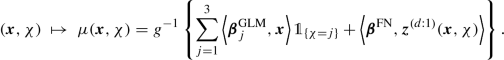
The indicator
 chooses the GLM that belongs to the corresponding insurance portfolio χ ∈{1, 2, 3} with the (individual) GLM parameter \(\boldsymbol {\beta }_{\chi }^{\text{GLM}}\). The FN network term makes them related, i.e., the GLMs of the different insurance portfolios interact (jointly learn) via the FN network module. This is the approach used in Gabrielli et al. [149] to improve the chain-ladder reserving method by learning across different claims reserving triangles.

 chooses the GLM that belongs to the corresponding insurance portfolio χ ∈{1, 2, 3} with the (individual) GLM parameter
 The regression function (7.40) gives the structural form of the combined regression model, but there is a second important ingredient proposed by Wüthrich–Merz [394]. Namely, the gradient descent algorithm (7.15) for model fitting can be started in an initial network parameter \(\Phi ^{(0)}\in {\mathbb R}^{q_0+1+r}\) that corresponds to the MLE of the GLM. Denote by \(\widehat {\boldsymbol {\beta }}^{\text{GLM}}\) the MLE of the GLM part, only.
Choose the initial value of the gradient descent algorithm for the fitting of the combined regression model (7.40)

that is, initially, no signals traverse the FN network part because we set β FN ≡ 0.
Remarks 7.21.
-
Using the initialization (7.42), the gradient descent algorithm starts exactly in the optimal GLM. The algorithm then tries to improve this GLM w.r.t. the given loss function using the additional FN network features. If the loss substantially reduces during the gradient descent training, the GLM misses systematic structure and it can be improved, otherwise the GLM is already good (enough).
-
We can declare the MLE \(\widehat {\boldsymbol {\beta }}^{\text{GLM}}\) to be non-trainable. In that case the original GLM always remains in the combined regression model and it acts as an offset. If we declare the MLE \(\widehat {\boldsymbol {\beta }}^{\text{GLM}}\) to be non-trainable, we could choose a trainable credibility weight α ∈ (0, 1), see (7.41), which gradually reduces the influence of the GLM (if necessary).
Implementation of the general combined regression model (7.40) can be a bit cumbersome, see Listing 4 in Gabrielli et al. [149], but things can substantially be simplified by declaring the GLM part in (7.40) as being non-trainable, i.e., estimating β GLM by \(\widehat {\boldsymbol {\beta }}^{\text{GLM}}\) in the GLM, and then freeze this parameter. In view of (7.40) this simply means that we add an offset \(o_i= \langle \widehat {\boldsymbol {\beta }}^{\text{GLM}}, \boldsymbol {x}_i\rangle \) to the FN network that is treated as a prior difference between the different data points, we refer to Sect. 5.2.3.
Example 7.22 (Combined GLM and FN Network). We revisit the French MTPL claim frequency GLM of Sect. 5.3.4, and we boost model Poisson GLM3 with FN network features. For the FN architecture we use the structure depicted in Fig. 7.14, i.e., a FN network of depth d = 3 having (q 1, q 2, q 3) = (20, 15, 10) neurons, and using embedding layers of dimension b = 2 for the categorical feature components. Moreover, we declare the GLM part to be non-trainable which allows us to use the GLM as an offset in the FN network. Moreover, we apply bias regularization (7.33) to receive the balance property.
The results are presented in Table 7.7. A first observation is that using model Poisson GLM3 as an offset reduces the run time of gradient descent fitting because we start the algorithm already in a reasonable model. Secondly, as expected, the FN features decrease the loss of model Poisson GLM3, this indicates that there are systematic effects that are not captured by the GLM. The final combined and regularized model has roughly the same out-of-sample loss as the corresponding FN network, showing that this approach can be beneficial in run times, and the predictive power is similar to a pure FN network. \(\blacksquare \)
Example 7.23 (Improving Model Poisson GLM3). In this example we would like to explore the deficiencies of model Poisson GLM3 by boosting it with FN network features. We do this in a systematic way by only considering two (continuous) features components at a time in the FN network. That is, we consider the combined approach (7.40) with initialization (7.42), but as feature information for the network part, we only consider two components at a time. For instance, we start with the features \((1,\mathtt {Area}, \mathtt {VehPower}) \in \{1\} \times {\mathbb R}^2\) for the network part, and the remaining feature information is ignored in this step. This way we can test whether the marginal modeling of Area and VehPower is suitable in model Poisson GLM3, and whether a pairwise interaction in these two components is missing. We train this FN network starting from model Poisson GLM3 (and keeping this GLM part frozen). The decrease in the out-of-sample loss during the gradient descent training is shown in Fig. 7.15 (top-left). We observe that the loss remains rather constant over 100 training epochs. This tells us that the pair (Area, VehPower) is appropriately considered in model Poisson GLM3.

Exploring all pairwise interactions: out-of-sample losses over 100 gradient descent epochs for all pairs of the continuous feature components Area, VehPower, VehAge, DrivAge, BonusMalus, Density (the scale on the y-axis is identical in all plots)
Figure 7.15 gives all pairwise plots of the continuous feature components Area, VehPower, VehAge, DrivAge, BonusMalus, Density, the scale on the y-axis is identical in all plots. We observe that only the plots including the variable BonusMalus provide a bigger decrease in loss (in blue color in the colored version). This indicates that mainly this feature component is not modeled optimally in model Poisson GLM3, because boosting with a FN network finds systematic structure here that improves the loss of model Poisson GLM3. In model Poisson GLM3, the variable BonusMalus has been modeled log-linearly with an interaction term with DrivAge and (DrivAge)2, see (5.35). Table 7.8 shows the result if we add a FN network feature (7.40) for the pair (DrivAge, BonusMalus) to model Poisson GLM3. Indeed, we see that the resulting combined GLM-FN network model has the same GL as the full FN network approach. Thus, we conclude that model Poisson GLM3 performs fairly well and only the modeling of the pair (DrivAge, BonusMalus) should be improved. \(\blacksquare \)
7.4.4 Network Ensemble Learning
Ensemble learning is a popular way of expressing that one takes an average over different predictors. There are many established methods that belong to the family of ensemble learning, e.g., there is boostrap aggregating (called bagging) introduced by Breiman [51], there are random forests, and there is boosting. Random forests and boosting are mainly based on classification and regression trees (CARTs) and they belong to the most powerful machine learning methods for tabular data. These methods combine a family of predictors to a more powerful predictor. The present section is inspired by the bagging method of Breiman [51], and we perform network aggregating (called nagging).
7.4.4.1 Stochastic Gradient Descent Fitting of Networks
We have described that network calibration involves several elements of randomness. This in combination with early stopping leads to the non-uniqueness of reasonably good networks for prediction and pricing. We have discussed this based on Fig. 7.5, namely, for a given network architecture we have a continuum of comparably good models (w.r.t. the chosen objective function) that lie in the green area of Fig. 7.5. One SGD calibration picks one specific model from this green area, we also refer to Remarks 7.9. Of course, this is very unsatisfactory in insurance pricing because it implies that the selection of a price for an insurance policy has a substantial element of subjectivity (that cannot be explained to the customer). Naturally, we would like to combine models in the green area of Fig. 7.5, for instance, by performing some sort of integration over the models in the green area. Intuitively, this should lead to a very powerful predictive model because it diversifies the weaknesses of each individual model. This is exactly what we discuss in this section. Before doing so, we would first like to understand the different single calibrations of a given network architecture.
We consider the MTPL data of Example 7.12. We model this data with a Poisson FN network using embedding layers for the categorical features and using bias regularization (7.33) to guarantee the balance property to hold. For the FN network architecture we choose depth d = 3 with (q 1, q 2, q 3) = (20, 15, 10) FN neurons; this setup gives us the results on the last line of Table 7.5. We now repeat this procedure M = 1′600 times, using exactly the same FN network architecture, the same early stopping strategy, the same SGD method and the same batch size. We only change the seeds of the starting point \(\boldsymbol {\vartheta }^{(0)} \in {\mathbb R}^r\) of the SGD algorithm, the partitioning of the learning data \(\mathcal {L}\) into training data \(\mathcal {U}\) and validation data \(\mathcal {V}\), see Fig. 7.7, and the partitioning of the training data into the (mini-)batches.
The resulting 1′600 in-sample and out-of-sample deviance losses are presented in Fig. 7.16. We observe a considerable variation in these figures. The in-sample losses vary between 23.616 and 23.815 (mean 23.728), and the corresponding out-of-sample loss between 23.766 and 23.899 (mean 23.819), units are in 10−2; note that all network calibrations are bias regularized. The in-sample loss is an average over n = 610′206 (individual) unit deviance losses, and the out-of-sample an average over T = 67′801 unit deviance losses, see also Definition 4.24. Therefore, we expect an even much bigger variation on individual insurance policies. We are going to analyze this in more detail in this section.

Boxplots over 1′600 network calibrations only differing in the seeds for the SGD algorithm and the partitioning of the learning data: (lhs) in-sample losses on \(\mathcal {L}\) and (rhs) out-of-sample losses on \(\mathcal {T}\), the horizontal lines show the calibration chosen in Table 7.5; units are in 10−2
Before doing so, we would like to understand whether there is some dependence between the in-sample and the out-of-sample losses over the M = 1′600 runs of the SGD algorithm with different seeds. In Fig. 7.17 we provide a scatter plot of the out-of-sample losses vs. the in-sample losses. This plot is complemented by a cubic spline regression (in orange color). From this plot we conclude that the models with very small in-sample losses tend to over-fit, and the models with large in-sample losses tend to under-fit (always using the same early stopping rule). In view of these results we conclude that the chosen early stopping rule is sensible because on average it tends to provide the model with the smallest out-of-sample loss on \(\mathcal {T}\). Recall that we do not use \(\mathcal {T}\) during the SGD fitting, but only the learning data \(\mathcal {L}\) that is split into the training data \(\mathcal {U}\) and the validation data \(\mathcal {V}\) for exercising the early stopping, see Fig. 7.7.

Scatter plot of out-of-sample losses vs. in-sample losses for different seeds, the orange line gives a fitted cubic spline, and the cyan lines show the empirical means; units are in 10−2
Next, we study the estimated prices on the test data (out-of-sample)
For each run of the SGD algorithm we receive a different (early stopped) network parameter estimate \(\widehat {\boldsymbol {\vartheta }}^m \in {\mathbb R}^r\), 1 ≤ m ≤ M = 1′600. Using these parameter estimates we receive the estimated network regression functions, for 1 ≤ m ≤ M,
using the FN network of Listing 7.4 with network parameter \(\widehat {\boldsymbol {\vartheta }}^m\). Thus, for the out-of-sample policies 1 ≤ t ≤ T we receive the expected frequencies
Since we choose the seeds of the SGD runs at random we may (and will) assume that we have independence between the prices \((\widehat {\mu }^m_t)_{t\in \mathcal {T}}\) of the different runs 1 ≤ m ≤ M of the SGD algorithm. This allows us to estimate the average price and the coefficient of variation of these prices of a fixed insurance policy t over the different SGD runs

These (out-of-sample) coefficients of variation are illustrated in Fig. 7.18. We observe a considerable variation on some policies. The average coefficient of variation is roughly 10% (orange horizontal line, lhs). The maximal coefficient of variation is about 40%, thus, for this policy the individual prices \(\widehat {\mu }^m_t\) of the different SGD runs 1 ≤ m ≤ M fluctuate considerably around \(\bar {\mu }^{(1:M)}_t\). This now explains why we choose M = 1′600 SGD runs, namely, the averaging in (7.43) reduces the coefficient of variation on this policy to  , note that we have independence between the different SGD runs. Thus, by averaging we receive an acceptable influence of the variation of the individual SGD fittings.

Out-of-sample coefficients of variations Vcot on an individual policy level 1 ≤ t ≤ T over the 1′600 calibrations (lhs) scatter plot against the average estimated frequencies \(\bar {\mu }^{(1:M)}_t \) and (rhs) resulting histogram
Listing 7.9 The 10 policies (out-of-sample) with the largest coefficients of variation

Listing 7.9 shows the 10 policies (out-of-sample) with the largest coefficients of variations Vcot. These polices have in common that they belong to the lowest BonusMalus level, the drivers are very young, the cars are comparably old and they have a bigger vehicle power. From a practical point of view we should doubt these policies, since the information provided may not be correct. New drivers (at the age of 18) typically enter a bonus-malus scheme at level 100, and only after several accident-free years these drivers can reach a bonus-malus level of 50. Thus, policies as in Listing 7.9 should not exist, and our pricing framework has difficulties to (correctly) handle them. In practice, this needs further investigation because, obviously, there is a data issue, here.
7.4.4.2 Nagging Predictor
The previously observed variations of the prices motivate to average over the different models (network calibrations). This brings us to bagging introduced by Breiman [51]. Bagging is based on averaging/aggregating over several ‘independent’ predictions; this is done in three steps. In a first step, a model is fitted to the data \(\mathcal {L}\). In a second step, independent bootstrap samples \(\mathcal {L}^{\ast (m)}\) are generated from this fitted model; the independence has to be understood in a conditional sense, namely, the different bootstrap samples \(\mathcal {L}^{\ast (m)}\) are independent in m, given the data \(\mathcal {L}\). In the third step, for every bootstrap sample \(\mathcal {L}^{\ast (m)}\) one estimates a model \(\widehat {\mu }^m\), and averaging (7.43) provides the bagging predictor. Bagging is mainly a variance reduction technique. Note that if the fitted model of the first step has a bias, then likely the bootstrap samples \(\mathcal {L}^{\ast (m)}\) are biased, and so is the bagging predictor. Therefore, bagging does not help to reduce a potential bias. All these results have to be understood conditionally on the data \(\mathcal {L}\). If this data is atypical for the problem, so will the bootstrap samples be.
We can perform a similar analysis for the fitted networks, but we do not need to bootstrap, here, because the various elements of randomness in SGD fitting allow us to generate independent predictors \(\widehat {\mu }^m\), conditional on the data \(\mathcal {L}\). Averaging (7.43) over these predictors then provides us with the network aggregating (nagging) predictor \(\bar {\mu }^{(1:M)}\); we also refer to Dietterich [105] and Richman–Wüthrich [315] for this aggregation. Thus, we replace the bootstrap step by the different runs of the SGD algorithm. Both options provide independent predictors \(\widehat {\mu }^m\), conditional on the data \(\mathcal {L}\). However, there is a fundamental difference between bagging and nagging. Bagging generates new (bootstrap) samples \(\mathcal {L}^{\ast (m)}\) and, thus, bagging also involves randomness coming from sampling the new observations. Nagging always acts on the same sample \(\mathcal {L}\), and it only refits the model multiple times. Therefore, the latter will typically introduce less variation. Of course, bagging and nagging can be combined, and then the full expected GL can be estimated, we come back to this in Sect. 11.4, below. We do not sample new observations, here, because we would like to understand the variations implied by the SGD algorithm with early stopping on the given (fixed) data.
In Fig. 7.18 we have seen that we need nagging over 1′600 network calibrations so that the maximal coefficient of variation on an individual policy level is below 1% in our MTPL example. In this section we would like to understand the minimal out-of-sample loss that can be achieved by nagging on the (entire) test data set, and we would like to analyze its rate of convergence.
For this we define the sequence of nagging predictors
This allows us to study the out-of-sample losses on \(\mathcal {T}\) in the Poisson model for M ≥ 1
Remark 7.24. From Remarks 7.17 we know that the expected deviance GL of the estimated model is lower bounded by the expected deviance GL of the true data generating model; the difference is the conditional calibration. Within the family of Tweedie’s CP models Richman–Wüthrich [315] proved that, indeed, aggregating decreases monotonically the expected deviance GL of the estimated model (Proposition 2 of [315]), convergence is established (Proposition 3 of [315]), and the speed of convergence is provided using asymptotic normality (Proposition 4 of [315]). For the Gaussian square loss results we refer to Breiman [51] and Bühlmann–Yu [60].
We revisit Proposition 2 of Richman–Wüthrich [315] which has also been proved in Proposition 3.1 of Denuit–Trufin [103]. We only consider a single case in the next proposition and we drop the feature information x (because we can condition on X = x).
Proposition 7.25. Choose a response Y ∼ f(⋅;θ, v∕φ) belonging to Tweedie’s CP model having a power variance cumulant function κ = κ p with power variance parameter p ∈ [1, 2], see (2.17). Assume \(\widehat {\mu }\) is an estimator for the mean parameter \(\mu =\kappa ^{\prime }_p(\theta )>0\) satisfying \(\epsilon <\widehat {\mu } \le p/(p-1) \mu \), a.s., for some 𝜖 ∈ (0, p∕(p − 1)μ). Choose i.i.d. copies \(\widehat {\mu }^m\), m ≥ 1, of \(\widehat {\mu }\) being all independent of Y . We have for all M ≥ 1
Proof of Proposition 7.25. The lower bound on the right-hand side immediately follows from Theorem 4.19. For an estimate \(\widehat {\mu }>0\) we define the function, we also refer to (4.18) and we set for the canonical link \(h_p=(\kappa ^{\prime }_p)^{-1}\),
This is the part of the log-likelihood (and deviance loss) that depends on the canonical parameter \(\widehat {\theta }=h_p(\widehat {\mu })\), and replacing the observation Y by μ. Calculating the second derivative w.r.t. \(\widehat {\mu }\) provides for p ∈ [1, 2]
the last inequality uses that the square bracket is non-positive, a.s., under our assumptions on \(\widehat {\mu }\). Thus, ψ p is concave on the interval (0, p∕(p − 1)μ). We now focus on the inequalities for M ≥ 1. Consider the decomposition of the nagging predictor for M + 1

The predictors \(\bar {\mu }^{(-j)}\), j ≥ 1, are copies of \(\bar {\mu }^{(1:M)}\), though not independent ones. Using the function ψ p, the second term on the right-hand side has the same structure as the estimation risk function (4.14),

the second last step applies Jensen’s inequality to the concave function ψ p, and the last step follows from the fact that \(\bar {\mu }^{(-j)}\), j ≥ 1, are copies of \(\bar {\mu }^{(1:M)}\). □
Remarks 7.26.
-
Proposition 7.25 says that aggregation works, i.e., aggregating i.i.d. predictors leads to monotonically decreasing expected deviance GLs. In fact, if \(\widehat {\mu }\le 2 \mu \), a.s., we receive Tweedie’s forecast dominance by aggregating, restricted to the power variance parameters p ∈ [1, 2], see Definition 4.22.
-
The i.i.d. assumption can be relaxed, indeed, it is sufficient that every \(\bar {\mu }^{(-j)}\) in the above proof has the same distribution as \(\bar {\mu }^{(1:M)}\). This does not require independence between the predictors \(\widehat {\mu }^m\), m ≥ 1, but exchangeability is sufficient.
-
We need the condition \(\epsilon <\widehat {\mu } \le p/(p-1) \mu \), a.s., to ensure the monotonicity within Tweedie’s CP models. For the Poisson model p = 1 we can drop the upper bound, and we only need the lower bound to ensure the existence of the expected deviance GL. For p ∈ (1, 2] the upper bound is increasingly binding, in the gamma case p = 2 requiring \(\widehat {\mu } \le 2 \mu \), a.s.
-
Note that we do not require unbiasedness of \(\widehat {\mu }\) for μ in Proposition 7.25. Thus, at this stage, aggregating is a variance reduction technique.
-
If additionally we have unbiasedness of \(\widehat {\mu }\) for μ and a uniformly integrable upper bound on \(\bar {\mu }^{(1:M)}\), we can use Lebesgue’s dominated convergence theorem and the law of large numbers to prove
$$\displaystyle \begin{aligned} \lim_{M\to \infty}{\mathbb E}_\theta\left[\mathfrak{d}\left(Y,\bar{\mu}^{(1:M)}\right)\right]= {\mathbb E}_\theta\left[\lim_{M\to \infty}\mathfrak{d}\left(Y,\bar{\mu}^{(1:M)}\right)\right]= {\mathbb E}_\theta\left[\mathfrak{d}(Y,{\mu})\right]. \end{aligned} $$(7.45)The uniformly integrable upper bound is only needed in the Poisson case p = 1, because the other cases are covered by \(\epsilon <\widehat {\mu } \le p/(p-1) \mu \), a.s. Moreover, asymptotic normality can be established, we refer to Proposition 4 in Richman–Wüthrich [315].
We come back to our MTPL Poisson claim frequency example and its 1′600 network calibrations illustrated in Fig. 7.17. Figure 7.19 provides the out-of-sample portfolio losses \({\mathfrak D}(\mathcal {T}, \bar {\mu }^{(1:M)})\) of the resulting nagging predictors \((\bar {\mu }^{(1:M)}(\boldsymbol {x}^\dagger _t))_{1\le t \le T}\) for 1 ≤ M ≤ 40 in red color, and the corresponding 1 standard deviation confidence bounds in orange color. The blue horizontal dotted line shows the case M = 1 which exactly refers to the (first) bias regularized FN network \(\widehat {\mu }^{m=1}\) with embedding layers given in Table 7.5. Indeed, averaging over multiple networks improves the predictive model and the out-of-sample loss decreases over the first 2 ≤ M ≤ 10 nagging steps. After the first 10 steps the picture starts to stabilize which indicates that for this size of portfolio (and this type of problem) we need to average over roughly 10–20 FN networks to receive optimal predictive models on the portfolio level. For M →∞ the out-of-sample loss converges to the green horizontal dotted line in Fig. 7.19 of 23.783 ⋅ 10−2. These numbers are also reported on the last line of Table 7.9.

Out-of-sample losses \({\mathfrak D}(\mathcal {T}, \bar {\mu }^{(1:M)})\) of the nagging predictors \((\bar {\mu }^{(1:M)}(\boldsymbol {x}^\dagger _t))_{1\le t \le T}\) for 1 ≤ M ≤ 40; losses are in 10−2
Figure 7.20 provides the empirical auto-calibration property (7.39) of the nagging predictor \(\bar {\mu }^{(1:1600)}\); this is obtained completely analogously to Fig. 7.12. The nagging predictors are (already) bias regularized, and Fig. 7.20 supports that the auto-calibration property holds rather accurately.

Empirical auto-calibration (7.39) of the Poisson nagging predictor, the blue line shows the empirical density of \(v_i \bar {\mu }^{(1:1600)}(\boldsymbol {x}_i)\), 1 ≤ i ≤ n
At this stage, we have fully arrived at Breiman’s [53] two modeling cultures dilemma, see also Sect. 1.1. We have started from a parametric data model, and in order to boost its predictive performance we have combined such models in an algorithmic way. Working with many blended networks is not really practical, therefore, in such situations, a meta model can be fitted to the resulting nagging predictor.
7.4.4.3 Meta Model
Since working with M = 1′600 different FN networks is not practical, we fit a meta model to the nagging predictors \(\bar {\mu }^{(1:M)}(\cdot )\). This can easily be done by just selecting an additional FN network and fit this additional network to the working data
For this calibration step we can consider all data, since we would like to fit a regression model as accurately as possible to the entire regression surface formed by all nagging predictors from the learning and the test data sets \(\mathcal {L}\) and \(\mathcal {T}\). Moreover, this step should not over-fit since this regression surface of nagging predictors does not include any noise, but it is on the level of expected values. As network architecture we choose again the same FN network of depth d = 3. The only change to the fitting procedure above is replacing the Poisson deviance loss by the square loss function, since we do not work with the Poisson responses N i but rather with their mean estimates \(\bar {\mu }^{(1:M)}(\boldsymbol {x}_i)\) and \(\bar {\mu }^{(1:M)}(\boldsymbol {x}^\dagger _t)\) in this fitting step. Since the resulting meta network model may still have a bias we apply the bias regularization step of Listing 7.7 to the Poisson observations with the Poisson deviance loss on the learning data \(\mathcal {L}\) (only). The results are presented in Table 7.10.
From these results we observe that in our case the meta network performs similarly well to the nagging predictor, and it seems to be a very reasonable choice.
Finally, in Fig. 7.21 (lhs) we analyze the resulting frequencies on an individual policy level on the test data set \(\mathcal {T}\). We plot the estimated frequencies \(\widehat {\mu }^{m=1}(\boldsymbol {x}_t^\dagger )\) of the first FN network (this corresponds to ‘embed FN bias regularized’ in Table 7.10 with an out-of-sample loss of 23.824) against the nagging predictor \(\bar {\mu }^{(1:M)}(\boldsymbol {x}_t^\dagger )\) which averages over M = 1′600 networks. From Fig. 7.21 (lhs) we conclude that there are quite some differences between these two predictors, this exactly reflects the variations obtained in Fig. 7.18 (lhs). The nagging predictor removes this variation by averaging. Figure 7.21 (rhs) compares the nagging predictor \(\bar {\mu }^{(1:M)}(\boldsymbol {x}_t^\dagger )\) to the one of the meta model \(\widehat {\mu }^{\text{meta}}(\boldsymbol {x}_t^\dagger )\). This scatter plot shows that the predictors lie almost perfectly on the diagonal line which suggests that the meta model can be used as a substitute for the nagging predictor. This completes this claim frequency modeling example.

Scatter plot of the out-of-sample predictions \(\widehat {\mu }^{m=1}(\boldsymbol {x}_t^\dagger )\), \(\bar {\mu }^{(1:M)}(\boldsymbol {x}_t^\dagger )\) and \(\widehat {\mu }^{\text{meta}}(\boldsymbol {x}_t^\dagger )\) over all polices 1 ≤ t ≤ T on the test data set \(\mathcal {T}\): (lhs) \(\widehat {\mu }^{m=1}(\boldsymbol {x}_t^\dagger )\) vs. \(\bar {\mu }^{(1:M)}(\boldsymbol {x}_t^\dagger )\) and (rhs) \(\widehat {\mu }^{\text{meta}}(\boldsymbol {x}_t^\dagger )\) vs. \(\bar {\mu }^{(1:M)}(\boldsymbol {x}_t^\dagger )\); the color scale shows the exposures \(v^\dagger _t \in (0,1]\)
Remark 7.27. The meta model concept can also be useful in other situations. For instance, we can fit a gradient boosting regression model to the observations. Typically, this is much faster than calculating a nagging predictor (because it directly focuses on the weaknesses of the existing model). If the gradient boosting model is based on regression trees, it has the disadvantage that the resulting regression function is not continuous, and a non-constant extrapolation might be an issue. In a second step we can fit a meta FN network model to the former regression model, lifting the boosting model to a smooth network that allows for a non-constant extrapolation. Example 7.28 (Gamma Claim Size Modeling). We revisit the gamma claim size example of Sect. 5.3.7. The data comprises Swedish motorcycle claim amounts. We have seen that this claim size data is not heavy-tailed, thus, a gamma distribution may be a reasonable choice for this data. For the modeling of this data we use the same normalization is in (5.45), this parametrization does not require the explicit knowledge of the (constant) shape parameter of the gamma distribution for mean estimation.
The difficulty with this data is that only 656 insurance policies suffer a claim, and likely a single FN network will not lead to stable results in this example. As FN network architecture we again choose a network of depth d = 3 and with (q 1, q 2, q 3) = (20, 15, 10) neurons. Since the input layer has dimension q 0 = 1 + 6 = 7 we receive a network parameter of dimension r = 626. As loss function we choose the gamma deviance loss, see Table 4.1. Moreover, we choose the nadam optimizer, a batch size of 300, a training-validation split of 8:2, and we retrieve the network calibration with the lowest validation loss with a callback.
Figure 7.22 shows the results of 1′000 different SGD runs (only differing in the initial seeds and the splits of the training-validation sets as well as the batches). We see a considerable variation between the different SGD runs, both in in-sample deviance losses but also in the average estimated claims. Note that we did not bias-regularize the resulting networks (we work with the log-link here which is not the canonical one). This is why we receive fluctuating portfolio averages in Fig. 7.22 (rhs), the red line illustrates the empirical mean. Obviously, these FN networks are (on average) positively biased, and they will need a bias correction for the final prediction.

Boxplots over 1′000 network calibrations only differing in the seeds for the SGD algorithm and the partitioning of the learning-validation data: (lhs) in-sample losses on the (entire) data \(\mathcal {L}\) and (rhs) average estimated claims
Figure 7.23 analyzes the variations on an individual claim level by studying the in-sample version of the coefficient of variation given in (7.43). We see that these coefficients of variation are bigger than in the claim frequency example, see Fig. 7.18. Thus, to receive stable results the nagging predictors \(\bar {\mu }^{(1:M)}(\boldsymbol {x}_i) \) have to be calculated over many networks. Figure 7.24 confirms that aggregating reduces (in-sample) losses also in this case. From this figure we also see that the convergence is slower compared to the MTPL frequency example of Fig. 7.19, of course, because we have a much smaller claims portfolio.

Coefficients of variations Vcoi on an individual claim level 1 ≤ i ≤ n over the 1′000 calibrations (lhs) scatter plot against the nagging predictor \(\bar {\mu }^{(1:M)}(\boldsymbol {x}_i) \) and (rhs) histogram

In-sample losses \({\mathfrak D}(\mathcal {L}, \bar {\mu }^{(1:M)})\) of the nagging predictors \((\bar {\mu }^{(1:M)}(\boldsymbol {x}_i))_{1\le i \le n}\) for 1 ≤ M ≤ 40 on the motorcycle claim size data
Table 7.11 presents the results if we take the nagging predictor over 1′000 different networks. The first observation is that we receive a much smaller in-sample loss compared to the GLMs, thus, there seems to be much room for improvements in the GLMs. Secondly, the nagging predictor has a substantial bias. For this reason we shift the intercept parameter in the output layer so that the portfolio average of the nagging predictor is equal to the empirical mean, see the last column of Table 7.11.
A main difficulty in this model is the estimation of the dispersion parameter φ > 0 and the shape parameter α = 1∕φ of the gamma distribution, respectively. Pearson’s dispersion estimate does not work because we do not know the degrees of freedom of the nagging predictor, see also (5.49). In Table 7.11 we calculate Pearson’s dispersion estimate by simply dividing by the number of observations; this should be understood as a lower bound; this number is highlighted in italic. Alternatively, we can calculate the MLE, however, this may be rather different from Pearson’s estimate, as indicated in Table 7.11. Figure 7.25 (lhs) shows the resulting QQ plot of the nagging predictor if we use the MLE \(\widehat {\varphi }^{\text{MLE}}=1.240\), and the right-hand side shows the same plot for \(\widehat {\varphi }=1.050\). From these plots it seems that we should rather go for a smaller dispersion parameter, the MLE being probably too much dominated by the small claims. This observation should also be understood as a red flag, as it tells us that the chosen gamma model is not fully suitable. This may be for various reasons: (1) the dispersion is not constant and should be modeled policy dependent, (2) the features are not sufficient to explain the observations, or (3) the gamma distribution is not suitable and should be replaced by another distribution.

QQ plots of the nagging predictors against the gamma density with (lhs) \(\widehat {\varphi }^{\text{MLE}}=1.240\) and (rhs) \(\widehat {\varphi }=1.050\)
In Fig. 7.26 (lhs) we compare the predictions received from model Gamma GLM2 against the nagging predictors \(\bar {\mu }^{(1:M)}(\boldsymbol {x}_i)\) over all instances 1 ≤ i ≤ n. The scatter plot spreads quite wildly around the diagonal which seriously questions at least one of the two models. To ensure that this variability between the two models is not caused by the (complex) FN network architecture, we verify the nagging predictor \(\bar {\mu }^{(1:M)}\), M = 1′000, by computing a second independent one. Indeed, Fig. 7.26 shows that these two independent nagging predictors come to the same conclusion on the individual instance level. Thus, the network finds/uses systematic effects that are not present in model Gamma GLM2. If we perform a pairwise interaction analysis for boosting the GLM as in Example 7.23, we find that we should add interactions to the GLM between (VehAge, RiskClass), (VehAge, BonusClass), (OwnerAge,Area), and (OwnerAge, VehAge); recall that model Gamma GLM2 neither includes BonusClass nor Gender as supported by a drop1 backward elimination analysis from model Gamma GLM1. However, it turns out, here, that we should have BonusClass in the model by letting it interact with VehAge.

(lhs) Scatter plot of model Gamma GLM2 predictors against the nagging predictors \(\bar {\mu }^{(1:M)}(\boldsymbol {x}_i)\) over all instances 1 ≤ i ≤ n, (rhs) scatter plot of two (independent) nagging predictors
Finally, Fig. 7.27 shows the empirical auto-calibration behavior (7.39) of the Gamma FN network nagging predictor of Table 7.11. The resulting black dots are rather volatile which shows that we do not (fully) have the auto-calibration property, here, but it also expresses that we fit a model on only 656 claims. The prediction of these claims is highlighted by the blue empirical density given by \(\bar {\mu }^{(1:M)}(\boldsymbol {x}_i)\), 1 ≤ i ≤ n. On the positive side, the auto-calibration plot shows that we neither systematically under- nor over-estimate because the black dots fluctuate around the diagonal red line, only the upper tail seems to under-estimate the true claim size. \(\blacksquare \)

7.4.4.4 Ensembling over Selected Networks vs. All Networks
Zhou et al. [406] ask the question whether ensembling over ‘selected’ networks is better than ensembling over all networks. In their proposal they introduce a weighted averaging scheme over the different network predictors \(\widehat {\mu }^m\), 1 ≤ m ≤ M. We perform a slightly different analysis here. We are re-using the M = 1′600 SGD calibrations of the Poisson FN network illustrated in Fig. 7.17. We order these SGD calibrations w.r.t. their in-sample losses \({\mathfrak D}(\mathcal {L}, \widehat {\mu }^m)\), 1 ≤ m ≤ M, and partition this ordered sample into three equally sized sets: the first one containing the smallest in-sample losses, the second one the middle sized in-sample losses, and the third one the largest in-sample losses. Figure 7.28 shows the empirical density of these in-sample losses, and the vertical lines give the partition into the three sets, we call the resulting (disjoint) index sets \(\mathcal {I}^{\text{small}}, \mathcal {I}^{\text{middle}}, \mathcal {I}^{\text{large}} \subset \{1,\ldots , M\}\). Remark that this partition is done fully in-sample, based on the learning data \(\mathcal {L}\), only.

Empirical density of the in-sample losses \({\mathfrak D}(\mathcal {L}, \widehat {\mu }^m)\), 1 ≤ m ≤ M, of Fig. 7.17
We then consider the nagging predictors on each of these index sets separately, i.e.,
If we believe into the orange cubic spline in Fig. 7.17, the middle nagging predictor \(\bar {\mu }^{\text{middle}}\) should out-perform the other two nagging predictors. Indeed, this is the case, here. We receive the out-of-sample losses (in 10−2) on the three subsets
This approach boosts by far any other approach considered, see Table 7.10; note that this analysis relies on a fully proper in-sample and out-of-sample testing strategy. Moreover, this also supports our early stopping strategy because, obviously, the optimal networks are centered around our early stopping rule. How does this result match Proposition 7.25 saying that the nagging predictor has a monotonically decreasing deviance loss. For the convergence (7.45) we need unbiasedness, and (7.47) indicates that averaging over all M network calibrations results in biases on an individual policy level; on the aggregate portfolio level, we have applied the bias regularization step (7.33), but this does not act on an individual policy level. The latter would require a local balance correction similar to the GAM approach presented in Example 7.19.
Figure 7.29 is truly striking! It compares the nagging predictors \(\bar {\mu }^{(1:M)}(\boldsymbol {x}_t^\dagger )\) to the ones \(\bar {\mu }^{\text{middle}}(\boldsymbol {x}^\dagger _t)\) only using the calibrations \(m\in \mathcal {I}^{\text{middle}}\), i.e., only using the calibrations with middle sized in-sample losses. The different colors show the exposures \(v_t^\dagger \in (0,1]\). We observe that only portfolios with short exposures do not lie on the diagonal line. Thus, there seems to be an issue with insurance policies with short exposures. Recall that we model the Poisson claim counts N i using the assumption, see (5.27),

Scatter plot of the nagging predictors \(\bar {\mu }^{\text{middle}}(\boldsymbol {x}^\dagger _t)\) and \(\bar {\mu }^{(1:M)}(\boldsymbol {x}_t^\dagger )\) over all out-of-sample polices 1 ≤ t ≤ T; the color scale shows the sizes of the exposures \(v_t^\dagger \in (0,1]\)
That is, the expected claim count \({\mathbb E}_{\theta _i}[N_i]=v_i \mu (\boldsymbol {x}_i)\) is assumed to scale proportionally in the exposure v i > 0. Figure 7.29 raises some doubts whether this is really the case, or at least SGD fitting has some difficulties to assess the expected frequencies μ(x i) on the policies i with short exposures v i > 0. We discuss this further in the next subsection. Table 7.12 gives a summary of our results.
7.4.4.5 Analysis of Over-dispersion
With all the excitement of Fig. 7.29, the above models do not fit the observations since the over-dispersion is too large, see the last column of Table 7.12. This has motivated the study of the negative binomial model in Sect. 5.3.5, the ZIP model in Sect. 5.3.6, and the hurdle Poisson model in Example 6.19. These models have led to an improvement in terms of AIC, see Table 6.6. We could go down the same route here by substituting the Poisson model. We refrain from doing so, as we want to further analyze the Poisson model. Suppose we calculate an AIC value for the Poisson FN network using 792 as the number of parameters involved. In that case, we receive a value of 191′790, thus, clearly lower than the one of the negative binomial GLM, and also slightly lower than the one of the hurdle Poisson model, see Table 6.6. Remark that AIC values within FN networks are not supported by any theory as we neither use the MLE nor do we have a reasonable evaluation of the number of parameters involved in networks. Thus, such a value may serve at best as a rough rule of thumb.
This lower AIC value suggests that we should try to improve the modeling of the systematic effects by better regression functions. In particular, there may be more explanatory variables involved that have predictive power. If these explanatory variables are latent, we can rely on the negative binomial model, as it can be interpreted as a mixture model averaging over latent variables. In view of Fig. 7.29, the exposures v i seem to have a predictive power different from proportional scaling, see (7.48); we also mention some peculiarities of the exposures on page 556. This motivates to change the FN network regression model such that the exposures are considered non-proportionally. We choose a FN network that directly models the mean of the claim counts
modeling the mean \({\mathbb E}_{\boldsymbol {\vartheta }}[N] =\mu (\boldsymbol {x}, v)\) of the Poisson datum (N, x, v). The expected frequency is then given by \({\mathbb E}_{\boldsymbol {\vartheta }}[Y]={\mathbb E}_{\boldsymbol {\vartheta }}[N/v]=\mu (\boldsymbol {x}, v)/v\).
Remark 7.29. At this stage we clearly have to distinguish between statistical modeling and actuarial modeling. In statistical modeling it makes perfect sense to choose the regression function (7.49), since including the exposure in a non-proportional way may increase the predictive power of the model, at least this is what our data suggests.
From an actuarial point of view this approach should clearly be doubted. The typical exposure of car insurance policies is one calendar year, i.e., v = 1, if the renewals of insurance policies are accounted correctly. Shorter exposures may have a specific (non-predictable) reason, for example, the policyholder or the insurance company may terminate an insurance contract after a claim. Thus, if this is possible, the exposure is a random variable, too, and it clearly has a predictive power for claims prediction; in that case we lose the properties of the Poisson count process (having independent and stationary increments).
As a consequence, we should include the exposure proportionally from an actuarial modeling point of view. Nevertheless we do the modeling exercise based on the regression function (7.49), here. This will indicate the predictive power of the exposure, which may be thought of a proxy for another (non-available) explanatory variable. Moreover, if (7.49) allows for a good Poisson regression model, we have a simple way of bootstrapping from our data (conditionally on given exposures v).
We would also like to emphasize that if one feature component dominates all others in terms of the predictive power, then likely there is a leakage of information through this component, and this needs a more careful analysis.
We implement the FN network regression model (7.49) using again a network architecture of depth d = 3 with (q 1, q 2, q 3) = (20, 15, 10) neurons. We use embedding layers for the two categorical variables VehBrand and Region, and we have 8 continuous/binary feature components. This is one more compared to Fig. 7.9 (rhs) because we also model the exposure v i as a continuous input to the network. As a result, the dimension r of the network parameter \(\boldsymbol {\vartheta } \in {\mathbb R}^r\) increases from 792 to 812 (because we have q 1 = 20 neurons in the first FN layer). We calculate the nagging predictor \(\bar {\mu }^{(1:M)}\) of this network averaging over M = 500 individual (early stopped) FN network calibrations, the results are presented in Table 7.13.
We observe a major improvement when including the exposure v as an input to the network, i.e., by including the exposure non-proportionally into the mean estimate. This is true in-sample (we use early stopping here), and in terms of Pearson’s dispersion estimate; we set r = 812 for the number of parameters in Pearson’s dispersion estimate (5.30) which may be too big because we do not perform proper MLE, here. In particular, we receive a dispersion estimate close to one which, now, is in support of modeling the claim counts by Poisson random variables (using this regression function). That is, this regression function explains the systematic effects so that we no longer observe much over-dispersion in the data relative to the chosen model. However, we would like to remind of Remark 7.29 which needs a careful consideration for the use of this regression model in insurance practice.
This is also supported by Fig. 7.30 which studies the average frequency as a function of the exposure v ∈ (0, 1]. The red observed average frequency has a clear decreasing slope which can be modeled by running the exposure v through the FN network (black), but not by including it proportionally (blue). From an actuarial modeling point of view this plot clearly questions the quality of the data, because there seem to be effects in the exposures that certainly require more investigation. Unfortunately, we cannot do this here because we do not have additional insight into this data set. This closes the example.

Average frequency as a function of the exposure v ∈ (0, 1]: nagging predictors considering the exposures proportionally (blue), the model including exposures non-proportionally through the FN network (black) and observed (red)
7.4.5 Identifiability in Feed-Forward Neural Networks
In the previous section we have studied ensembles of FN networks. One may also aim at directly comparing these networks to each other in terms of the fitted network parameters \(\widehat {\boldsymbol {\vartheta }}^{j}\) over the different calibrations 1 ≤ j ≤ M (of the same FN network architecture). Such a comparison may, e.g., be useful if one wants to choose a prior parameter distribution π for 𝜗 in a Bayesian setting. Comparing the different network calibrations \(\widehat {\boldsymbol {\vartheta }}^{j}\), 1 ≤ j ≤ M, of an architecture needs some care because networks have many symmetries that make the parameters non-identifiable. We can, for instance, permute the neurons in a FN layer z (m), with the corresponding permutation of the weights that connect this layer to the previous layer z (m−1) and to the succeeding layer z (m+1). The resulting predictive model under this permutation is the same as the original one. For this reason we need to introduce some order in a FN network to make the parameters identifiable.
Rüger–Ossen [323] have introduced the notion of a fundamental domain for the network parameter 𝜗, and we briefly review this idea. We start with an explicit example. Assume that the activation function fulfills the anti-symmetry property − ϕ(x) = ϕ(−x) for all \(x\in {\mathbb R}\), this is the case for the hyperbolic tangent. This implies several symmetries in the FN network parametrization. E.g., if we consider the output of a shallow FN network d = 1 with link function g, we can do a sign switch in a fixed neuron 1 ≤ k ≤ q 1
From this we see that the following two network parameters (we switch signs in all the parameters that belong to index k)

give the same FN network predictions. Beside these sign switches, we can also permute the enumeration of the neurons in a given FN layer, giving the same predictions. We discuss Theorem 2 of Rüger–Ossen [323] to solve this identifiability issue. First, we consider the network weights from the input x to the first FN layer z (1)(x). Apply the sign switch operation (7.50) to the neurons in the first FN layer so that all the resulting intercepts \(w^{(1)}_{0,1}, \ldots , w^{(1)}_{0,q_1}\) are positive while not changing the regression function x↦g(μ(x)). Next, apply a permutation to the indices 1 ≤ j ≤ q 1 so that we receive ordered intercepts
with an unchanged regression function x↦g(μ(x)). To make these transformations well-defined we need to assume that all intercepts are non-zero and mutually different (which we assume for the time-being).
Then, we move recursively through the FN layers 2 ≤ m ≤ d applying the sign switch operations and the permutations so that the regression function x↦g(μ(x)) remains unchanged and such that for all 1 ≤ m ≤ d
This provides us with a unique representation of every network parameter \(\boldsymbol {\vartheta }\in {\mathbb R}^r\) in the fundamental domain
supposed that all intercepts are different from zero and mutually different in the same FN layers. As stated in Section 2.2 of Rüger–Ossen [323], there may still exist different parameters in this fundamental domain that provide the same predictive model, but these are of zero Lebesgue measure. The same applies to the intercepts \(w^{(m)}_{0,j}\) being zero or having equal intercepts for different neurons. Basically, this means that we are fine if we work with absolutely continuous prior distributions on the fundamental domain when we want to work within a Bayesian setup.
7.5 Auto-encoders
Auto-encoders are tools that aim at reducing the dimension of high-dimensional data such that the reconstruction error of the original data is small, i.e., such that the loss of information by the dimension reduction is minimized. The most popular auto-encoder is the principal components analysis (PCA) which we are going to present here. The PCA is a linear dimension reduction technique. Bottleneck neural (BN) networks can be viewed as a non-linear extension of the PCA. This is going to be discussed in Sect. 7.5.5, below. Dimension reduction techniques belong to the family of unsupervised learning methods because they do not consider a response variable, but they aim at finding common structure in the features. Unsupervised learning methods can roughly be categorized into three classes: dimension reduction techniques (studied in this section), clustering methods and visualization methods. For a discussion of clustering and visualization methods we refer to the tutorial of Rentzmann–Wüthrich [310].
7.5.1 Standardization of the Data Matrix
Assume we have q-dimensional data points \(\boldsymbol {y}_i \in {\mathbb R}^q\), 1 ≤ i ≤ n. This provides us with a data matrix

We assume that each of the q columns of Y measures a quantity in a given unit. The first column may, for instance, describe the age of a car driver in years, the second column his body weight in kilograms, etc. That is, each column 1 ≤ j ≤ q of Y describes a specific quantity, and each row  of Y describes these quantities for a given instance 1 ≤ i ≤ n. Since often the analysis should not depend on the units of the columns of Y , one centers the columns with the empirical means \(\bar {y}_j=\sum _{i=1}^n y_{i,j}/n\), and one normalizes them with the empirical standard deviations \(\widehat {\sigma }_j=(\sum _{i=1}^n (y_{i,j}-\bar {y}_j)^2/n)^{1/2}\), 1 ≤ j ≤ q. This gives the normalized data matrix

We typically center the data matrix Y , providing \(\sum _{i=1}^n y_{i,j}=0\) for all 1 ≤ j ≤ q, normalization w.r.t. the standard deviation can be done, but is not always necessary. Centering implies that we can interpret Y as a q-dimensional empirical distribution with each component (column) being centered. The covariance matrix of this (centered) empirical distribution is calculated as

This is a covariance matrix, and if the columns of Y are normalized with the empirical standard deviations \(\widehat {\sigma }_j\), 1 ≤ j ≤ q, this is a correlation matrix.
7.5.2 Introduction to Auto-encoders
An auto-encoder encodes a high-dimensional vector \(\boldsymbol {y} \in {\mathbb R}^q\) to a low-dimensional representation so that the dimension reduction leads to a minimal loss of information. A function \(L(\cdot ,\cdot ):{\mathbb R}^q\times {\mathbb R}^q \to {\mathbb R}_+\) is called dissimilarity function if L(y, y ′) = 0 if and only if y = y ′.
An auto-encoder is a pair ( Φ, Ψ) of mappings, for given dimensions p < q,
such that their composition Ψ ∘ Φ has a small reconstruction error w.r.t. the chosen dissimilarity function L(⋅, ⋅), that is,
Note that we want (7.55) for selected cases y, and if they are within a p-dimensional manifold the auto-encoding will be successful. The first mapping \(\Phi : {\mathbb R}^q \to {\mathbb R}^p\) is called encoder, and the second mapping \(\Psi : {\mathbb R}^p \to {\mathbb R}^q\) is called decoder. The object \(\Phi (\boldsymbol {y})\in {\mathbb R}^p\) is a p-dimensional encoding (representation) of \(\boldsymbol {y} \in {\mathbb R}^q\) which contains maximal information of y up to the reconstruction error (7.55).
7.5.3 Principal Components Analysis
PCA gives us a linear auto-encoder (7.54). If the data matrix \(\boldsymbol {Y} \in {\mathbb R}^{n\times q}\) has rank q, there exist q linearly independent rows of Y that span \({\mathbb R}^q\). PCA determines a different, very specific basis of \({\mathbb R}^q\). It looks for an orthonormal basis \(\boldsymbol {v}_1,\ldots , \boldsymbol {v}_q\in {\mathbb R}^q\) such that v 1 explains the direction of the biggest variability in Y , v 2 the direction of the second biggest variability in Y orthogonal to v 1, and so forth. Variability is understood in the sense of maximal empirical variance under the assumption that the columns of Y are centered, see (7.52)–(7.53). Such an orthonormal basis can be found by determining q linearly independent eigenvectors of the symmetric and positive definite matrix

For this we can solve recursively the following convex Lagrange problems. The first basis vector \(\boldsymbol {v}_1 \in {\mathbb R}^q\) is determined by the solution ofFootnote 3

and the j-th basis vector \(\boldsymbol {v}_j \in {\mathbb R}^q\), 2 ≤ j ≤ q, is received recursively by the solution of

Singular value decomposition (SVD) gives an alternative way of computing this orthonormal basis, we refer to Section 14.5.1 in Hastie et al. [183]. The algorithm of Golub–Van Loan [165] gives an efficient way of performing a SVD. There exist orthogonal matrices \(U\in {\mathbb R}^{n\times q}\) and \(V \in {\mathbb R}^{q\times q}\) (with  ), and a diagonal matrix \(\Lambda = \mbox{diag}(\lambda _1,\ldots , \lambda _q)\in {\mathbb R}^{q\times q}\) with singular values λ
1 ≥… ≥ λ
q > 0 such that we have the SVD
), and a diagonal matrix \(\Lambda = \mbox{diag}(\lambda _1,\ldots , \lambda _q)\in {\mathbb R}^{q\times q}\) with singular values λ
1 ≥… ≥ λ
q > 0 such that we have the SVD

The matrix U is called left-singular matrix of Y , and the matrix V is called right-singular matrix of Y . Observe by using the SVD (7.58)

That is, the squared singular values \((\lambda ^2_j)_{1\le j \le q}\) are the eigenvalues of matrix A, and the column vectors of the right-singular matrix V = (v 1, …, v q) (eigenvectors of A) give an orthonormal basis v 1, …, v q. This motivates to define the q principal components of Y by the column vectors of
E.g., the first principal component of the instances 1 ≤ i ≤ n is given by \(\boldsymbol {Y}\boldsymbol {v}_1=\lambda _1 \boldsymbol {u}_{1} \in {\mathbb R}^n\). Considering the first p ≤ q principal components gives the rank p matrix

The Eckart–Young–Mirsky theorem [114, 279]Footnote 4 proves that this rank p matrix Y p minimizes the Frobenius norm relative to Y among all rank p matrices, that is,

where the Frobenius norm is given by \(\|C\|{ }_{\text{F}}^2={\sum _{i,j}c_{i,j}^2}\) for a matrix C = (c i,j)i,j.
The orthonormal basis \(\boldsymbol {v}_1,\ldots , \boldsymbol {v}_q \in {\mathbb R}^q\) gives the (linear) encoder (projection)

These gives the first p principal components in (7.59) if we insert the transposed data matrix  for \(\boldsymbol {y} \in {\mathbb R}^{q}\). The (linear) decoder Ψ is given by
The following is understood column-wise for the transposed data matrix  ,
,

Thus,  minimizes the Frobenius reconstruction error (7.61) on the data matrix
  among all linear maps of rank p. In view of (7.55) we can express the squared Frobenius reconstruction error as
thus, we choose the squared Euclidean distance as the dissimilarity measure, here, that we minimize simultaneously on all cases y i, 1 ≤ i ≤ n.
Remark 7.30. The PCA gives a linear approximation to the data matrix Y by minimizing (7.61) and (7.62) for given rank p. This may not be appropriate if the non-linear terms are dominant. Figure 7.31 (lhs) gives a situation where the PCA works well; this data has been generated by i.i.d. multivariate Gaussian random vectors \(\boldsymbol {y}_i\sim \mathcal {N}(\boldsymbol {0}, \Sigma )\). Figure 7.31 (middle) gives a non-linear example where the PCA does not work well, the data matrix \(\boldsymbol {Y} \in {\mathbb R}^{n\times 2}\) is a column-centered matrix that builds a circle around the origin.

Two-dimensional PCAs in different situations of the data matrix \(\boldsymbol {Y} \in {\mathbb R}^{n\times 2}\)
Another nice example where the PCA fails is Fig. 7.31 (rhs). This figure is inspired by Shlens [337] and Ruckstuhl [321]. It shows a situation where the level sets are non-convex, and the principal components point into a completely wrong direction to explain the structure of the data.
7.5.4 Lab: Lee–Carter Mortality Model
We use the SVD to fit the most popular stochastic mortality model, the Lee–Carter (LC) model [238], to (raw) mortality data. The raw mortality data considers for each calendar year t and each age x the number of people D x,t who died (in that year t at age x) divided by the corresponding population exposure e x,t. In practice this requires some care. Due to migration, often, the exposures e x,t are non-observable figures and need to be estimated. Moreover, also the death counts D x,t in year t at age x can be defined differently, age cohorts are usually defined by the year of birth. We denote the (observed) raw mortality rates by M x,t = D x,t∕e x,t. The subsequent derivations consider the raw log-mortality rates log(M x,t), for this reason we assume that M x,t > 0 for all calendar years t and ages x. The goal is to model these raw log-mortality rates (for each country, region, risk group and gender separately).
The LC model defines the force of mortality as
where log(μ x,t) is the (deterministic) log-mortality rate in calendar year t for a person aged x (for a fixed country, region and gender). The individual terms in (7.63) have the following meaning: a x is the average force of mortality at age x, b x is the rate of change of the force of mortality broken down to the different ages x, and k t is the time index describing the change of the force of mortality in calendar year t.
Strictly speaking, we do not have a stochastic model, here, that can explain the observations M x,t, but we try to fit a deterministic mortality surface (μ x,t)x,t to these noisy observations (M x,t)x,t. For this we use the PCA and the Frobenius norm as the measure of dissimilarity (on the log-scale).
In a first step, we center the raw log-mortality rates for all ages x, i.e., over the calendar years \(t\in \mathcal {T}\) under consideration. We define the centered raw log-mortality rates y x,t and the estimate \(\widehat {a}_x\) of the average force of mortality at age x as follows
where the last identity defines the estimate \(\widehat {a}_x\). Strictly speaking we have a slight difference to the centering in Sect. 7.5.1 because we center the rows and not the columns of the data matrix, here, but the role of rows and columns is exchangeable in the PCA. The optimal (parameter) values \((\widehat {b}_x)_x\) and \((\widehat {k}_t)_t\) are determined as follows, see (7.63),

where the sum runs over the years \(t \in \mathcal {T}\) and the ages x 0 ≤ x ≤ x 1, with x 0 and x 1 being the lower and upper age boundaries. This can be rewritten as an optimization problem (7.61)–(7.62). Consider the data matrix \(\boldsymbol {Y}=(Y_{x,t})_{x_0\le x \le x_1; t \in \mathcal {T}} \in {\mathbb R}^{n\times q}\), and set n = x 1 − x 0 + 1 and \(q=|\mathcal {T}|\). Assume Y has rank q. This allows us to consider

A solution to this problem is given, see (7.60),

with left-singular matrix \(U=(\boldsymbol {u}_1,\ldots , \boldsymbol {u}_q) \in {\mathbb R}^{n\times q}\) and right-singular matrix \(V=(\boldsymbol {v}_1,\ldots , \boldsymbol {v}_q) \in {\mathbb R}^{q\times q}\) of Y . This implies that the first principal component \(\lambda _1 \boldsymbol {u}_1=\boldsymbol {Y} \boldsymbol {v}_1 \in {\mathbb R}^n\) gives an estimate for \((b_x)_{x_0\le x \le x_1}\), and the first column vector \(\boldsymbol {v}_1 \in {\mathbb R}^q\) of V gives an estimate for the time index \((k_t)_{t \in \mathcal {T}}\). For parameter identifiability we normalize
the latter being consistent with the centering of the rows of Y with \(\widehat {a}_x\) in (7.64).
We fit the LC model to the Swiss mortality data of females and males separately. The raw log-mortality rates log(M x,t) for the years \(t \in \mathcal {T}=\{1950, \ldots , 2016\}\) and the ages 0 ≤ x ≤ 99 are illustrated in Fig. 7.32; both plots use the same color scale. This mortality data has been obtained from the Human Mortality Database (HMD) [195]. In general, we observe a diagonal structure that indicates mortality improvements over time.

Raw log-mortality rates log(M x,t) for the calendar years 1950 ≤ t ≤ 2016 and the ages x 0 = 0 ≤ x ≤ x 1 = 99 of Swiss females (lhs) and Swiss males (rhs); both plots use the same color scale
Define the fitted log-mortality surface
Figure 7.33 shows the LC fitted log-mortality surface \(({\mbox{log}}(\widehat {\mu }_{x,t}))_{0\le x \le 99; t \in \mathcal {T}}\) separately for Swiss females and Swiss males, the color scale is the same as in Fig. 7.32. The plots show a huge similarity between the raw log-mortality data and the LC fitted log-mortality surface which clearly supports the LC model for the Swiss data. In general, the LC surface is a smoothed version of the raw log-mortality surface. The main difference in our LC fit concerns the male population for ages 20 ≤ x ≤ 40 from 1980 to 2000, one explanation of the special pattern in the observed data during that time is the emergence of HIV.

LC fitted log-mortality rates \({\mbox{log}}(\widehat {\mu }_{x,t})\) for the calendar years 1950 ≤ t ≤ 2016 and the ages x 0 = 0 ≤ x ≤ x 1 = 99 of Swiss females (lhs) and Swiss males (rhs); the plots use the same color scale as Fig. 7.32
Figure 7.34 (lhs) shows the singular values \(\lambda _1 \ge \ldots \ge \lambda _{|\mathcal {T}|}>0\) for Swiss females and Swiss males. We observe that the first singular value λ 1 by far dominates the remaining singular values λ j, j ≥ 2. Thus, the first principal component indeed may already be sufficient, and the centered raw log-mortality data Y can be described by a matrix Y 1 of rank p = 1. Figure 7.34 (rhs) gives the squared Frobenius reconstruction errors of the approximations Y p of ranks \(0\le p \le |\mathcal {T}|\), where Y 0 corresponds to the zero matrix where we do not use any approximation, but use just the average observed log-mortality rate. We observe that the first singular value leads by far to the biggest decrease in the reconstruction error, and the subsequent expansions λ j, j ≥ 2, improve it only slightly in each step. This supports the use of the LC model using a rank p = 1 approximation to the centered raw log-mortality rates Y . The higher rank PCA within mortality modeling has been studied in Renshaw–Haberman (RH) [308], and the RH(p) mortality model considers the rank p approximation Y p to the raw log-mortality rates Y given by
for \(\boldsymbol {b}_x, \boldsymbol {k}_t \in {\mathbb R}^p\).

(lhs) Singular values λ j, \(1\le j \le |\mathcal {T}|\), of the SVD of the data matrix \(\boldsymbol {Y} \in {\mathbb R}^{n\times |\mathcal {T}|}\), and (rhs) the reconstruction errors \(\| \boldsymbol {Y}-\boldsymbol {Y}_p\|{ }^2_{\text{F}}\) for \(0\le p \le |\mathcal {T}|\)
We have (only) fitted a mortality surface to the raw log-mortality rates on the rectangle \(\{x_0, \ldots , x_1\} \times \mathcal {T}\). This does not allow us to forecast mortality into the future. Forecasting requires a two step procedure, which, after this first estimation step, extrapolates the time index (time-series) \((\widehat {k}_t)_{t \in \mathcal {T}}\) beyond the latest observation point in \(\mathcal {T}\). The simplest (meaningful) model for this second (extrapolation) step is a random walk with drift for the time index process \((\widehat {k}_t)_{t \ge 0}\). Figure 7.35 shows the estimated two-dimensional process \((\widehat {\boldsymbol {k}}_t)_{t \in \mathcal {T}}\), i.e., for p = 2, on the rectangle \(\{x_0, \ldots , x_1\} \times \mathcal {T}\) which needs to be extrapolated to predict within the RH (p = 2) mortality model. We refrain from doing this step, but extrapolation will be studied in Sect. 8.4, below.

Estimated two-dimensional processes \((\widehat {\boldsymbol {k}}_t)_{t \in \mathcal {T}}\) for Swiss females (lhs) and Swiss males (rhs); these are normalized such that they are centered and such that the components of \(\widehat {\boldsymbol {b}}_x\) add up to 1
7.5.5 Bottleneck Neural Network
BN networks have become popular in studying non-linear generalizations of PCA, we refer to Kramer [225] and Hinton–Salakhutdinov [186]. The BN network architecture is such that (1) the input dimension q 0 is equal to the output dimension q d+1 of a FN network, and (2) in between there is a FN layer 1 ≤ m ≤ d that has a very low dimension q m ≪ q 0, called the bottleneck. Figure 7.36 (lhs) shows such a BN network of depth d = 3 and neurons
The input and output neurons have blue color, and the bottleneck of dimension q 2 = 2 is shown in red color in Fig. 7.36 (lhs).

(lhs) BN network of depth d = 3 with (q 0, q 1, q 2, q 3, q 4) = (20, 7, 2, 7, 20), (middle and rhs) shallow BN networks with a bottleneck of dimensions 7 and 2, respectively
The motivation is as follows. Assume we have a given dissimilarity function \(L(\cdot ,\cdot ):{\mathbb R}^q\times {\mathbb R}^q \to {\mathbb R}_+\) that measures the reconstruction error of an auto-encoder \(\Psi \circ \Phi (\boldsymbol {y})\in {\mathbb R}^q\) relative to the original input \(\boldsymbol {y} \in {\mathbb R}^q\), see (7.55). We try to find a BN network with input and output dimensions q 0 = q d+1 = q (we drop the intercepts in the entire construction) and a bottleneck in layer m having a low dimension q m, such that the BN network provides a small reconstruction error. Choose a FN network
with FN layers for 1 ≤ m ≤ d (excluding intercepts)

and having network weights \(\boldsymbol {w}_j^{(m)} \in {\mathbb R}^{q_{m-1}}\), 1 ≤ j ≤ q m. For the output we choose the identity function as activation function

and having network weights \(\boldsymbol {w}_j^{(d+1)} \in {\mathbb R}^{q_{d}}\), 1 ≤ j ≤ q
d+1. The resulting network parameter 𝜗 is now fitted to the data matrix  such that the reconstruction error is minimized over all instances

We use this fitted network parameter \(\widehat {\boldsymbol {\vartheta }}\) and denote the resulting FN layers by \(\widehat {\boldsymbol {z}}^{(m)}\) for 1 ≤ m ≤ d + 1.
This allows us to define the BN encoder, set q = q 0 and p = q m,
and the BN decoder is given by, set q m = p and q d+1 = q,
The BN encoder (7.66) gives us a q
m-dimensional representation of the data. A linear rank p representation Y
p of Y , see (7.61), can be found by a BN network architecture that has a minimal FN layer width of dimension p =min1≤j≤d
q
j, and with the identity activation function ϕ(x) = x. Such a BN network is a linear map of maximal rank p. Using the Euclidean square distance as dissimilarity measure provides us an optimal network parameter \(\widehat {\boldsymbol {\vartheta }}\) for this linear map such that we receive  . There is one point to be considered, here, why the bottleneck activations \(\Phi (\boldsymbol {y})= \widehat {\boldsymbol {z}}^{(m:1)}(\boldsymbol {y}) \in {\mathbb R}^p\) in the linear activation case are not directly comparable to the principal components
  of the PCA. Namely, the PCA uses an orthonormal basis v
1, …, v
p whereas the linear BN network case uses any p-dimensional basis, i.e., to directly bring these two representations in line we still need a coordinate transformation of the bottleneck activations.
of the PCA. Namely, the PCA uses an orthonormal basis v
1, …, v
p whereas the linear BN network case uses any p-dimensional basis, i.e., to directly bring these two representations in line we still need a coordinate transformation of the bottleneck activations.
Hinton–Salakhutdinov [186] noticed that the gradient descent fitting of a BN network needs some care, otherwise we may find a local minimum of the loss function that has a poor reconstruction performance. In order to implement a more sophisticated way of SGD fitting we require that the depth d of the network is an odd number and that the network architecture is symmetric around the central FN layer (d + 1)∕2. This is the case in Fig. 7.36 (lhs). Fitting of this network of depth d = 3 is now done in three steps:
-
1.
The symmetry around the central FN layer m = 2 allows us to collapse this central layer by merging layers 1 and 3 (because q 1 = q 3). Merging these two layers provides us a shallow BN network with neurons (q 0, q 1 = q 3, q d+1 = q 0) = (20, 7, 20). This shallow BN network is shown in Fig. 7.36 (middle). In a first step we fit this simpler network to the data Y . This gives us the preliminary estimates for the network weights \(\boldsymbol {w}_1^{(1)}, \ldots , \boldsymbol {w}_{q_1}^{(1)}\) and \(\boldsymbol {w}_1^{(4)}, \ldots , \boldsymbol {w}_{q_4}^{(4)}\) of the full BN network. From this fitted shallow BN network we receive the learned representations \(\boldsymbol {z}_i=\boldsymbol {z}^{(1)}(\boldsymbol {y}_i) \in {\mathbb R}^{q_1}\), 1 ≤ i ≤ n, in the central layer using the preliminary estimates of the network weights.
-
2.
In the second step we use the learned representations \(\boldsymbol {z}_i \in {\mathbb R}^{q_1}\), 1 ≤ i ≤ n, to fit the inner part of the original network (using a suitable dissimilarity function). This inner part is a shallow network with neurons (q 1, q 2, q 3 = q 1) = (7, 2, 7), see Fig. 7.36 (rhs). This second step gives us the preliminary estimates for the network weights \(\boldsymbol {w}_1^{(2)}, \ldots , \boldsymbol {w}_{q_2}^{(2)}\) and \(\boldsymbol {w}_1^{(3)}, \ldots , \boldsymbol {w}_{q_3}^{(3)}\) of the full BN network.
-
3.
In the final step we fit the full BN network on the data Y and use the preliminary estimates of the weights (of the previous two steps) as initialization of the gradient descent algorithm.
Example 7.31 (BN Network Mortality Model). We apply this BN network approach to modify the LC model of Sect. 7.5.4. Hainaut [178] considered such a BN network application. For computational reasons, Hainaut [178] proposed a calibration strategy different from Hinton–Salakhutdinov [186]. We use this latter calibration strategy as it has turned out to work well in our setting.
As BN network architecture we choose a FN network of depth d = 3. The input and output dimensions are equal to q 0 = q 4 = 67, this exactly corresponds to the number of available calendar years 1950 ≤ t ≤ 2016, see Fig. 7.32. Then, we select a symmetric architecture around the central FN layer m = 2 with q 1 = q 3 = 20 neurons. That is, in a first step, the 67 calendar years are compressed to a 20-dimensional representation. For the bottleneck we then explore different numbers of neurons q 2 = p ∈{1, …, 20}. These BN networks are implemented and fitted in R with the library keras [77]. We have fitted these models separately to the Swiss female and male populations. The raw log-mortality rates are illustrated in Fig. 7.32, and for comparability with the LC approach we have centered these log-mortality rates according to (7.64), and we use the squared Euclidean distance as the objective function.
Figure 7.37 compares the squared Frobenius reconstruction errors of the linear LC approximations Y p to their non-linear BN network counterparts with bottlenecks q 2 = p. We observe that the BN figures are clearly smaller saying that a non-linear auto-encoding provides a better reconstruction, this is true, in particular, for 2 ≤ q 2 < 20. For q 2 ≥ 20 the learning with the BN networks seems saturated, note that the outer layers have q 1 = q 3 = 20 neurons which limits the learning at the bottleneck for bigger q 2. In view of Fig. 7.37 there seems to be a kink at q 2 = 4, and an “elbow” criterion says that this is the critical bottleneck size that should not be exceeded.

Frobenius reconstruction errors \(\| \boldsymbol {Y}-\boldsymbol {Y}_p\|{ }^2_{\text{F}}\) for 1 ≤ p = q 2 ≤ 20 in the linear LC approach and the non-linear BN approach
The resulting estimated log-mortality surfaces for the bottleneck q 2 = 2 are illustrated in Fig. 7.38. These strongly resemble the raw log-mortality rates in Fig. 7.32, in particular, for the male population we get a better fit for ages 20 ≤ x ≤ 40 from 1980 to 2000 compared to the LC model. In a further analysis we should check whether this BN network does not over-fit to the data. We could, e.g., explore drop-outs during calibration or smaller FN (compression) layers q 1 = q 3.

BN network (q 1, q 2, q 3) = (20, 2, 20) fitted log-mortality rates \({\mbox{log}}(\widehat {\mu }_{x,t})\) for the calendar years 1950 ≤ t ≤ 2016 and the ages x 0 = 0 ≤ x ≤ x 1 = 99 of Swiss females (left) and Swiss males (right); the plots use the same color scale as Fig. 7.32
Finally, we analyze the resulting activations at the bottleneck by considering the BN encoder (7.66). Note that we assume \(\boldsymbol {y} \in {\mathbb R}^q\) in (7.66) with \(q=|\mathcal {T}|\) being the rank of the data matrix \(\boldsymbol {Y} \in {\mathbb R}^{n\times q}\). Thus, the encoder takes a fixed age 0 ≤ x ≤ 99 and encodes the corresponding time-series observation \(\boldsymbol {y}_x \in {\mathbb R}^{|\mathcal {T}|}\) by the bottleneck activations. This parametrization has been inspired by the PCA which typically considers a data matrix that has more rows than columns. This results in at most q = rank(Y ) singular values, supposed n ≥ q. However, we can easily exchange the role of rows and columns, e.g., by transposing all matrices involved. For mortality forecasting it is advantageous to exchange these roles because we would like to extrapolate a time-series beyond \(\mathcal {T}\). For this reason we set for the input dimension q 0 = q = 100, which provides us with \(|\mathcal {T}|\) observations \(\boldsymbol {y}_t \in {\mathbb R}^{100}\). We then fit the BN encoder (7.66) to receive the bottleneck activations
Figure 7.39 shows these figures for a bottleneck q 2 = 2. We observe that these bottleneck time-series \((\Phi (\boldsymbol {y}_t))_{t \in \mathcal {T}}\) are much more difficult to understand than the LC/RH ones given in Fig. 7.35. Firstly, we see that we have quite some dependence between the components of the time-series. Secondly, in contrast to the LC/RH case of Fig. 7.35, there is not one component that dominates. Note that this dominance has been obtained by scaling the components of (b x)x to add up to 1 (which, of course, reflects the magnitudes of the singular values). In the non-linear case, these scales are hidden in the decoder which is more difficult to extract. Thirdly, the extrapolation may not work if the time-series has a trend and if we use the hyperbolic tangent activation function that has a bounded range. In general, a trend extrapolation has to be considered very carefully with FN networks with non-linear activation functions, and often there is no good solution to this problem within the FN network framework. We conclude that this approach improves in-sample mortality surface modeling, but it leaves open the question about forecasting the future mortality rates because an extrapolation seems more difficult. \(\blacksquare \) Remark 7.32. The concept of BN networks has also been considered in the actuarial literature to encode geographic information, see Blier-Wong et al. [39]. Since geographic information has a natural spatial component, these authors propose to use a convolutional neural network to encode the spatial information before processing the learned features through a BN network. The proposed decoder may have different forms, either it tries to reconstruct the whole (spatial) neighborhood of a given location or it only tries to reconstruct the site of a given location.

BN network (q 1, q 2, q 3) = (20, 2, 20): bottleneck activations showing \(\Phi (\boldsymbol {y}_t) \in {\mathbb R}^2\) for \(t \in \mathcal {T}\)
7.6 Model-Agnostic Tools
We collect some model-agnostic tools in this section that help us to better understand and analyze the networks, their calibrations and predictions. Model-agnostic tools are techniques that are not specific to a certain model type and can be used for any regression model. Most methods presented here are nicely presented in the tutorial of Lorentzen–Mayer [258]. There are several ways of getting a better understanding of a regression model. First, we can analyze variable importance which tries to answer similar questions to the GLM variable selection tools of Sect. 5.3 on model validation. However, in general, we cannot rely on any asymptotic likelihood theory for such an analysis. Second, we can try to understand the predictive model. For a GLM with the log-link function this is quite simple because the systematic effects are of a multiplicative nature. For networks this is much more complicated because we allow for much more general regression functions. We can either try to understand these functions on a global portfolio level (by averaging the effects over many insurance policies) or we can try to understand these functions locally for individual insurance policies. The latter refers to local sensitivities around a chosen feature value \(\boldsymbol {x} \in \mathcal {X}\), and the former to global model-agnostics.
7.6.1 Variable Permutation Importance
For GLMs we have studied the LRT and the Wald test that have been assisting us in reducing the GLM by the feature components that do not contribute sufficiently to the regression task at hand, see Sects. 5.3.2 and 5.3.3. These variable reduction techniques rely on an asymptotic likelihood theory. Here, we need to proceed differently, and we just aim at ranking the variables by their importance, similarly to a drop1 analysis, see Listing 5.6.
For a given FN network regression model
we randomize one component of  at a time, and we study the resulting change in the objective function. More precisely, for given (learning) data \(\mathcal {L}\), with features x
1, …, x
n, we select one feature component 1 ≤ j ≤ q and permute (x
i,j)1≤i≤n randomly across the entire portfolio 1 ≤ i ≤ n. We denote by \(\mathcal {L}^{(j)}\) the resulting data with the j-th component being permuted. We then compare the resulting deviance loss \({\mathfrak D}(\mathcal {L}^{(j)}, \mu )\) to the one \({\mathfrak D}(\mathcal {L}, \mu )\) on the original data \(\mathcal {L}\) using the same regression model μ. We call this approach variable permutation importance (VPI). Note that such a permutation does not only act on the marginal effects, but it also distorts the interaction effects of the different feature components.
at a time, and we study the resulting change in the objective function. More precisely, for given (learning) data \(\mathcal {L}\), with features x
1, …, x
n, we select one feature component 1 ≤ j ≤ q and permute (x
i,j)1≤i≤n randomly across the entire portfolio 1 ≤ i ≤ n. We denote by \(\mathcal {L}^{(j)}\) the resulting data with the j-th component being permuted. We then compare the resulting deviance loss \({\mathfrak D}(\mathcal {L}^{(j)}, \mu )\) to the one \({\mathfrak D}(\mathcal {L}, \mu )\) on the original data \(\mathcal {L}\) using the same regression model μ. We call this approach variable permutation importance (VPI). Note that such a permutation does not only act on the marginal effects, but it also distorts the interaction effects of the different feature components.
We calculate the VPI on the MTPL claim frequency data of model Poisson GLM3 of Table 5.5 and the FN network regression model \(\widehat {\mu }^{m=1}\) of Table 7.9; we use this example throughout this section on model-agnostic tools. Figure 7.40 shows the relative increases
of the deviance losses by permuting one feature component 1 ≤ j ≤ q at a time.

Obviously, the BonusMalus level followed by DrivAge and VehBrand are the most important variables according to this VPI method. This is in alignment for both models. Thereafter, there are smaller disagreements between the two models. These disagreements may (also) be caused by a non-optimal feature pre-processing in the GLM where, for instance, we have to add the interaction effects manually, see (5.35). Overall, these VPI results are in line with the findings of the classical methods on GLMs, see for instance the drop1 table in Listing 5.6.
One point that is worth mentioning (and which makes the VPI results not fully reliable) is the use of feature components that are highly correlated. In our case, Density and Area are highly correlated, see Fig. 13.12. Therefore, it may not make sense to randomly permute one component while keeping the other one unchanged. This issue will also arise in other methods described below. Remark 7.33 (Global Surrogate Model). There are other machine learning methods that offer different measures of variable importance. For instance, (binary split) classification and regression trees (CARTs) offer popular methods for measuring variable importance; for binary split CARTs we refer to Breiman et al. [54] and Denuit et al. [100]. These CARTs select individual feature components for partitioning the feature space \(\mathcal {X}\), and variable importance is measured by analyzing the contribution of each feature component to the total decrease of the objective function. Binary split CARTs have the advantage that this can be done in an additive way.
More complex regression models like FN networks can then be analyzed by using a binary split regression tree as a global surrogate model. That is, we can fit a CART to the network regression function (as a surrogate model) and then analyze variable importance in this surrogate regression tree model using the tools of regression trees. We will not give an explicit example here because we have not formally introduced regression trees in this manuscript, but this concept is fairly straightforward and well-understood.
7.6.2 Partial Dependence Plots
There are several graphical tools that study the individual behavior in the feature components. Some of these tools select individual insurance policies and others study global portfolio properties. They have in common that they are based on marginal considerations, i.e., some sort of projection.
7.6.2.1 Individual Conditional Expectation
Individual conditional expectation (ICE) selects individual insurance policies (Y i, x i, v i) and varies the feature components of x i over their entire domain; we refer to Goldstein et al. [164]. Similarly to the VPI of Sect. 7.6.1, ICE does not respect collinearity in feature components, but it is rather an isolated view of individual components.
In Fig. 7.41 we provide the ICE plots of model Poisson GLM3 of Table 5.5 and the FN network regression model \(\widehat {\mu }^{m=1}\) of Table 7.9 of 100 randomly selected insurance policies x i. For these randomly selected insurance policies we let the variable DrivAge vary over its domain {18, …, 90}. Each color corresponds to one insurance policy i, and the colors in the two plots coincide. In the GLM we observe that the lines are roughly parallel which reflects that we have an additive regression structure on the canonical scale (note that these plots are on the canonical parameter scale). The lines are not perfectly parallel because we allow for an interaction between DrivAge and BonusMalus in model Poisson GLM3, see (5.35). The plot of the FN network is more difficult to interpret. Overall the levels (colors) coincide in the two plots, but in the FN network plot the lines are not increasing for ages approaching 18, the reason for this is that we have interactions with other feature components that are important. In particular, for ages close to 18 we cannot have a BonusMalus level of 50% and, therefore, the FN network cannot be trained on this part of the feature space. Nevertheless, the ICE plot allows for such feature configurations (by just extrapolating the FN network regression function beyond the set of available insurance policies). This difficulty is confirmed by exploiting the same plot only on insurance policies that have a BonusMalus level of at least 100%. In that case the lines for small ages are non-decreasing when approaching the age of 18, thus, providing a more reasonable interpretation. We conclude that if we have strong dependence and/or interactions between the feature components this method may not provide any reasonable interpretations.

ICE plots of 100 randomly selected insurance policies x i of (lhs) model Poisson GLM3 and (rhs) FN network \(\widehat {\mu }^{m=1}\) letting the variable DrivAge vary over its domain; the y-axis is on the canonical parameter scale
7.6.2.2 Partial Dependence Plot
Partial dependence plots (PDPs) have been introduced by Friedman [141], see also Zhao–Hastie [405]. PDPs are closely related to the do-operator in causal inference in statistics; we refer to Pearl [298] and Pearl et al. [299] for the do-operator. A PDP and the do-operator, respectively, are obtained by breaking the dependence structure between different feature components. Namely, we decompose the feature x = (x j, x ∖j) into two parts with x ∖j denoting all feature components except of component x j; we will use a slight abuse of notation because the components need to be permuted correspondingly in the following regression function x → μ(x) = μ(x j, x ∖j). Since, typically, there is dependence between x j and x ∖j one can infer x ∖j from x j, and vice versa. A PDP breaks this inference potential so that the sensitivity can be studied purely in x j. In particular, the partial dependence profile is obtained by
where p(x ∖j) is the marginal (portfolio) distribution of the feature components x ∖j. Observe that this differs from the conditional expectation which reads as
the latter allowing for inferring x ∖j from x j through the conditional probability dp(x ∖j|x j).
Remark 7.34 (Discrimination-Free Insurance Pricing). Recent actuarial literature discusses discrimination-free insurance pricing which aims at developing a pricing framework that is free of discrimination w.r.t. so-called protected characteristics such as gender and ethnicity; we refer to Guillén [174], Chen et al. [69, 70], Lindholm et al. [253] and Frees–Huang [136] for discussions on discrimination in insurance. In general, part of the problem also lies in the fact that one can often infer the protected characteristics from the non-protected feature information. This is called indirect discrimination or proxy discrimination. The proposal of Lindholm et al. [253] for achieving discrimination-free prices exactly follows the construction (7.67), by breaking the link, which infers the protected characteristics from the non-protected ones.
The partial dependence profile on our portfolio \(\mathcal {L}\) with given features x 1, …, x n is now obtained by just using the portfolio distribution as an empirical distribution for p in (7.67). That is, for a selected component x j of x, we consider the partial dependence profile
thus, we average the ICE plots over x i,∖j of our portfolio 1 ≤ i ≤ n.
Figure 7.42 (lhs, middle) give the PDPs of the variables BonusMalus and DrivAge of model Poisson GLM3 and the FN network \(\widehat {\mu }^{m=1}\). Overall they look reasonable. However, we are again facing the difficulty that these partial dependence profiles consider feature configurations that should not appear in our portfolio. Roughly 57% of all insurance policies have a bonus-malus level of 50%, which means that these driver’s did not suffer any claims in the past couple of years. Obviously a driver of age 18 cannot be on this bonus-malus level, simply because she/he is not in a state where she/he can have multiple years of driving experience without an accident. However, the PDP does not respect this fact, and just extrapolates the regression function into that part of the feature space. Therefore, the PDP at driver’s age 18 is based on 57% of the insurance policies being on a bonus-malus level of 50% because this corresponds to the empirical portfolio distribution p(x ∖j) excluding the driver’s age x j = DrivAge information. Figure 7.42 (rhs) shows the ratio of insurance policies that have a bonus-malus level of 50%. We observe that this ratio is roughly zero up to age 28 (orange vertical dotted line), which indicates that a driver needs 10 successive accident-free years to reach the lowest bonus-malus level (starting from 100%). We consider it to be data error that this ratio below age 28 is not identically equal to zero. We conclude that these PDPs need to be interpreted very carefully because the insurance portfolio is not uniformly distributed across the feature space. In some parts of the feature space the regression function x↦μ(x) may not even be well-defined because certain combinations of feature values x may not exist (e.g., a driver of age 18 on bonus-malus level 50% or a boy at a girl’s college).

PDPs of (lhs) BonusMalus level and (middle) DrivAge; the y-axis is on the canonical parameter scale; (rhs) ratio of policies with a bonus-malus level of 50% per driver’s age
7.6.2.3 Accumulated Local Effects Profile
PDPs have the problem that they do not respect the dependencies between the feature components, as explained in the previous paragraphs. The accumulated local effects (ALE) profile tries to take account for these dependencies by only studying a local feature perturbation, we refer to Apley–Zhu [13]. We present a smooth (gradient-based) version of ALE because our regression functions are differentiable. Consider the local effect in the individual feature x w.r.t. the component x j by studying the partial derivative
The average local effect of component j is received by
ALE integrate the average local effects Δj(⋅) over their domain, and the ALE profile is defined by
where \({x_{j_0}}\) is a given initialization point. The difference between PDPs and ALE is that the latter correctly considers the dependence structure between x j and x ∖j, see (7.69).
Listing 7.10 Local effects through the gradients of FN networks in keras [77]

Example. We come back to our MTPL claim frequency FN network example. The local effects (7.68) can directly be calculated in the R library keras [77] for a FN network, see Listing 7.10. In order to do so we need to drop the embedding layers, compared to Listing 7.4, and directly work on the learned embeddings. This gives an input layer of dimension q = 7 + 2 + 2 = 11 because we have two categorical features that have been embedded into 2-dimensional Euclidean spaces \({\mathbb R}^2\). Then, we can formally calculate the gradient of the FN network w.r.t. its inputs which is done on lines 11–13 of Listing 7.10. Remark that we work on the canonical scale because we use the linear activation function on line 7 of the listing.
There remain the averaging (7.69) and the integration (7.70) which can be done empirically
where \(\mathcal {E}(x_j)\) denotes the indices i of all cases x i, 1 ≤ i ≤ n, with x i,j = x j, assuming of having discrete feature data observations. Note that this empirical averaging respects the dependence within x. The (uncentered) ALE profile is then obtained by aggregating these local effects, that is,
where this integration is typically understood in a discrete sense because the observed feature components x i,j are discrete. Often, this uncentered ALE profile is still translated (centered) by the portfolio average.
Remarks 7.35.
-
We have only introduced ALE for continuous feature variables. For nominal categorical feature components it is not immediately clear how to reasonably integrate the average local effects Δj(x j;μ), and one typically directly analyzes these average local effects.
-
For GLMs the ALEs are rather simple if we work on the canonical scale and under the canonical link, since
$$\displaystyle \begin{aligned} \theta_{j}(\boldsymbol{x}) = \frac{\partial \theta(\boldsymbol{x})}{\partial x_j} =\beta_j \equiv \Delta_j(x_j;\theta). \end{aligned}$$In the case of model Poisson GLM3 presented in Sect. 5.3.4 the situation is more delicate as we model the interactions in the GLM as follows, see (5.34) and (5.35),
$$\displaystyle \begin{aligned} \begin{array}{rcl} & &\displaystyle (\mathtt{DrivAge},\mathtt{BonusMalus}) \\ & &\displaystyle \quad \mapsto \beta_l\, \mathtt{DrivAge} +\beta_{l+1} {\mbox{log}}(\mathtt{DrivAge}) +\sum_{j=2}^4\beta_{l+j} (\mathtt{DrivAge})^j \\& &\displaystyle \qquad + \beta_{l+5}\mathtt{BonusMalus} + \beta_{l+6}~ \mathtt{BonusMalus} \cdot \mathtt{DrivAge} \\& &\displaystyle \qquad +\beta_{l+7}\mathtt{BonusMalus} \cdot (\mathtt{DrivAge})^2. \end{array} \end{aligned} $$In that case, though we work with a GLM, the resulting local effects are different if we calculate the derivatives w.r.t. DrivAge and BonusMalus, respectively, because we explicitly (manually) include non-linear effects into the GLM.
Figure 7.43 shows the ALE profiles of the variables BonusMalus and DrivAge. The shapes of these profiles can directly be compared to the PDPs of Fig. 7.42 (the scale on the y-axis should be ignored because this will depend on the applied centering, however, we hold on to the canonical scale). The main difference between these two plots can be observed for the variable DrivAge at low ages. Namely, the ALE profiles have a different shape at low ages respecting the dependencies in the feature components by only considering real local feature configurations.

ALE profiles of (lhs) BonusMalus level and (rhs) DrivAge; the y-axis is on the log-scale
7.6.3 Interaction Strength
Next we are going to discuss pairwise interaction strength. Friedman–Popescu [143] made the following proposal. Roughly speaking, there is an interaction between the two feature components x j and x k of x in the regression function x↦μ(x) if
This means that the magnitude of a change of the regression function μ(x) in x j depends on the current value of x k. If there is no such interaction, we can additively decompose the regression function μ(x) into two independent terms. This then reads as μ(x) = μ ∖j(x ∖j) + μ ∖k(x ∖k). This motivation is now applied to the PDP profiles given in (7.67). We define the centered versions x j↦μ̆j(x j) and x k↦μ̆k(x k) of the PDP profiles by centering the PDP profiles \(x_j \mapsto \bar {\mu }^j(x_j)\) and \(x_k \mapsto \bar {\mu }^k(x_k)\) over the portfolio values x i, 1 ≤ i ≤ n. Next, we consider an analogous two-dimensional version for (x j, x k). Let (x j, x k)↦μ̆j, k(x j, x k) be the centered version of a two-dimensional PDP profile \((x_j,x_k) \mapsto \bar {\mu }^{j,k}(x_j,x_k)\).
Friedman’s H-statistics measures the pairwise interaction strength between the components x j and x k, and it is defined by
we refer to formula (44) in Friedman–Popescu [143]. While \(H^2_{j,k}\) measures the proportion of the joint interaction effect, as we normalize by the variability of the joint effect \(\sum _{i=1}^n \breve {\mu }^{j,k}(x_{i,j},x_{i,k})^2\), sometimes also the absolute measure is considered by taking the square root of the enumerator in (7.73). Of course, this can be extended to interactions of three components, etc., we refer to Friedman–Popescu [143].
We do not give an example here, because calculating Friedman’s H-statistics can be computationally demanding if one has many feature components with many levels in FN network modeling.
7.6.4 Local Model-Agnostic Methods
The above methods like the PDP and the ALE profile have been analyzing the global behavior of the regression functions. We briefly mention some tools that describe the local sensitivity and explanation of regression results.
Probably the most popular method is the locally interpretable model-agnostic explanation (LIME) introduced by Ribeiro et al. [311]. This analyzes locally the expected response of a given feature x by perturbing x. In a nutshell, the idea is to select an environment \(\mathcal {E}(\boldsymbol {x}) \subset \mathcal {X}\) of a chosen feature x and to study the regression function x ′↦μ(x ′) in this environment \(\boldsymbol {x}' \in \mathcal {E}(\boldsymbol {x})\). This is done by fitting a (much) simpler surrogate model to μ on this environment \(\mathcal {E}(\boldsymbol {x})\). If the environment is small, often a linear regression model is chosen. This then allows one to interpret the regression function μ(⋅) locally using the simpler surrogate model, and if we have a high-dimensional feature space, this linear regression is complemented with LASSO regularization to only select the most important feature components.
The second method considered in the literature is the Shapley additive explanation (SHAP). The SHAP is based on Shapley values [335] which is a method of allocating rewards to players in cooperative games, where a team of individual players jointly contributes to a potential success. Shapley values solve this allocation problem under the requirements of additivity and fairness. This concept can be translated to analyzing how individual feature components of x contribute to the total prediction μ(x) of a given case. Shapley values allow one to do such a contribution analysis in the aforementioned additive and fair way, see Lundberg–Lee [261]. The calculation of SHAP values is combinatorially demanding and therefore several approximations have been proposed, many of them having their own caveats, we refer to Aas et al. [1]. We will not further consider these but refer to the relevant literature.
7.6.5 Marginal Attribution by Conditioning on Quantiles
The above model-agnostic tools have mainly been studying the sensitivities of the expected response μ(x) in the feature components of x. This becomes apparent from considering the partial derivatives (7.68) to calculate the local effects. Alternatively, we could try to understand how the feature components of x contribute to a given response μ(x), see Ancona et al. [12]; this section follows Merz et al. [273]. The marginal attribution on an input component j of the response μ(x) can be studied by the directional derivative
This was first proposed to the data science community by Shrikumar et al. [340]. Basically, it means that we replace the partial derivative μ
j(x) by the directional derivative along the vector 

where e j is the (j + 1)-st basis vector in \({\mathbb R}^{q+1}\) (index j = 0 corresponds to the intercept component x 0 = 1).
We start by recalling the sensitivity analysis of Hong [189] and Tsanakas–Millossovich [355] in the context of risk measurement. Assume the features have a portfolio distribution X ∼ p. This describes the random selection of an insurance policy X = x from the portfolio described by p. The average price over the entire portfolio is then given by
We implicitly interpret \(\mu (\boldsymbol {X})={\mathbb E}[Y|\boldsymbol {X}]\) as the price of the response Y , here, though we do not need the response distribution in this section. Assume μ(X) has a continuous distribution function F μ(X); and we drop the intercept component X 0 = x 0 = 1 from these considerations (but we still keep it in the regression model). This implies that U μ(X) = F μ(X)(μ(X)) is uniformly distributed on [0, 1]. Choosing a density ζ on [0, 1] gives us a probability distortion ζ(U μ(X)) as we have the normalization
This allows us to define a distorted portfolio price in the sense of a Radon–Nikodým derivative, namely, we set for the distorted portfolio price
This functional ϱ(μ(X);ζ) is a so-called distortion risk measure. Our goal is to study the sensitivities of this distortion risk measure in the components of X. Assume existence of the following directional derivatives for all 1 ≤ j ≤ q

S j(μ;ζ) can be used to describe the sensitivities of the regression function X↦μ(X) in the feature components X j. Under different sets of assumptions, Hong [189] and Tsanakas–Millossovich [355] have proved the following identity
the right-hand side exactly uses the marginal attribution (7.74). There remains the freedom of the choice of the density ζ on [0, 1], which allows us to study the sensitivities of different distortion risk measures. For the uniform distribution ζ ≡ 1 on [0, 1] we simply have the average (best-estimate) price and its average marginal attributions
If we want to consider a quantile risk measure, called value-at-risk (VaR), we choose a Dirac measure for the density ζ. That is, choose a point measure of mass 1 in α ∈ (0, 1), i.e., the density ζ is concentrated in the single point α. In that case, the event {F μ(X)(μ(X)) = U μ(X) = α} receives probability one, and therefore we have the α-quantile
and the corresponding sensitivities for 1 ≤ j ≤ q
Remarks 7.36.
-
In the introduction to this section we have assumed that μ(X) has a continuous distribution function. This emphasizes that this sensitivity analysis is most suitable for continuous feature components. Categorical and discrete feature components can be embedded into a Euclidean space, e.g., using embedding layers, and then they can be treated as continuous variables.
-
Sensitivities (7.75) respect the local portfolio structure as they are calculated w.r.t. p.
-
In applications, we will work with the empirical portfolio distribution for p provided by (x i)1≤i≤n. This gives an empirical approximation to (7.75) and, in particular, it will require a choice of a bandwidth for the evaluation of the conditional probability, conditioned on the event \(\{ \mu (\boldsymbol {X})=F_{\mu (\boldsymbol {X})}^{-1}(\alpha ) \}\). This is done with a local smoother similarly to Listing 7.8.
In analogy to Merz et al. [273] we give a different interpretation to the sensitivities (7.75), which allows us to further expand this formula. We have 1st order Taylor expansion

Obviously, this is a local approximation in x. Setting 𝜖 = −x, we get (a possibly crude) approximation

By bringing the gradient term to the other side, using (7.75) and conditionally averaging, we receive the 1st order marginal attributions
Thus, the sensitivities S j(μ;α) provide a 1st order description of the quantiles \(F_{\mu (\boldsymbol {X})}^{-1}(\alpha )\) of μ(X). We call this approach marginal attribution by conditioning on quantiles (MACQ) because it shows how the components X j of X contribute to a given quantile level.
Example 7.37 (MACQ for Linear Regression). The simplest case is the linear regression case because the 1st order marginal attributions (7.76) are exact in this case. Consider a linear regression function with regression parameter \(\boldsymbol {\beta } \in {\mathbb R}^{q+1}\)
The 1st order marginal attributions for fixed α ∈ (0, 1) are given by
That is, we replace the feature components X j by their expected contributions on a given quantile level \(F_{\mu (\boldsymbol {X})}^{-1}(\alpha )\) in (7.77). We compare this explanation to the ALE profile (7.70). Set initial value \({x_{j_0}}=0\), the ALE profile for the linear regression model is given by
This is the sensitivity of the linear regression function in component x j, whereas (7.77) describes the contribution of each feature component to an expected response level μ(x), in particular, \({\mathbb E}_p[X_j| \mu (\boldsymbol {X})=F_{\mu (\boldsymbol {X})}^{-1}(\alpha )]\) describes the average feature value in component j on a given quantile level. \(\blacksquare \)
A natural next step is to expand the 1st order attributions to 2nd orders. This allows us to consider the interaction terms. Consider the 2nd order Taylor expansion

Similar to (7.76), setting 𝜖 = −x, this gives us the 2nd order marginal attributions
where for 1 ≤ j, k ≤ q we define \(\mu _{j,k}(\boldsymbol {x})=\partial _{x_j}\partial _{x_k} \mu (\boldsymbol {x})\), see (7.72), and
Remarks 7.38.
-
The first line of (7.78) separates the 1st order attributions from the 2nd order attributions, the second line splits w.r.t. the individual component j attributions and the interaction attributions j ≠ k.
-
The 1st order attributions (7.75) have been motivated by considering the directional derivatives of the VaR distortion risk measure. Unfortunately, the 2nd order consideration has no simple equivalent motivation, as the 2nd order directional derivatives are much more involved, even in the linear case, we refer to Property 1 in Gourieroux et al. [167].
-
Interestingly, we can precisely evaluate the accuracy of approximation (7.78) by analyzing for a given regression function μ(⋅)
$$\displaystyle \begin{aligned} \sup_{\alpha \in (0,1)}\left| F_{\mu(\boldsymbol{X})}^{-1}(\alpha) -\mu\left(\boldsymbol{0}\right) - \sum_{j=1}^q S_j( \mu; \alpha) +\frac{1}{2} \sum_{j,k=1}^q T_{j,k}(\mu; \alpha) \right|. \end{aligned} $$(7.80)Intuitively, in order to have a uniform good approximation, the origin 0 should be somehow centered in the feature distribution X ∼ p. This will be studied next.
Above we have implicitly assumed that 0 is a suitable reference point that makes the approximation error (7.80) small. For FN network fitting we typically normalize the features either using the MinMaxScaler (7.29) or we center and normalize the components of (x i)1≤i≤n according to (7.30). That is, the reference point is chosen such that the gradient descent fitting works efficiently. However, this may not be an optimal reference point for studying the 2nd order attributions. Therefore, we analyze this question in more detail, and the following reparametrization can still be done after model fitting.
If we choose an arbitrary translation \(\boldsymbol {a} \in {\mathbb R}^q\), we can set 𝜖 = a −x in the above 2nd order Taylor expansion to receive another 2nd order marginal attribution representation

Essentially, this means that we shift the feature distribution p to considering the shifted random vectors X a = X −a and while setting μ a(⋅) = μ(a + ⋅), thus, this simply says that we pre-process the features differently. In view of approximation (7.81) we can now select a reference point \(\boldsymbol {a} \in {\mathbb R}^q\) that makes the 2nd order marginal attributions as precise as possible. Define the events \(\mathcal {A}_l=\{\mu (\boldsymbol {X})=F_{\mu (\boldsymbol {X})}^{-1}(\alpha _l)\}\) for a discrete quantile grid 0 < α 1 < … < α L < 1. We define the objective function

Making this objective function G(a;μ) small in a will provide us with a good reference point for the selected quantile levels (α l)1≤l≤L; this is exactly the MACQ proposal of Merz et al. [273]. A local minimum can be found by applying a gradient descent algorithm
for tempered learning rates δ t+1 > 0. The gradient of G w.r.t. a is given by

All subsequent considerations and interpretations are done w.r.t. an optimal reference point \(\boldsymbol {a} \in {\mathbb R}^q\) by minimizing the objective function (7.82) on the chosen quantile grid. Mathematically speaking, this optimal choice is w.l.o.g. because the origin 0 of the coordinate system of the feature space \(\mathcal {X}\) is arbitrary, and any other origin can be chosen by a translation, see formula (7.81) and the subsequent discussion. For interpretations, however, the choice of the reference point a matters because the directional derivative X j μ j(X) can be small either because X j is small or because μ j(X) is small. Having a small X j means that this feature value is close to the chosen reference point.
Example 7.39 (MACQ Analysis). We revisit the MTPL claim frequency example using the FN network regression model of depth d = 3 having (q 1, q 2, q 3) = (20, 15, 10) neurons. Importantly, we use the hyperbolic tangent as the activation function in the FN layers which provides smoothness of the regression function. Figure 7.40 shows the VPI plot of this fitted model. Obviously, the variable BonusMalus plays the most important role in this predictive model. Remark that the VPI plot does not properly respect the dependence structure in the features as it independently permutes each feature component at a time. The aim in this example is to determine variable importance by doing the MACQ analysis (7.78).
Figure 7.44 (lhs) shows the empirical density of the fitted canonical parameter θ(x i), 1 ≤ i ≤ n; all plots in this example refer to the canonical scale. We then minimize the objective function (7.82) which provides us with an optimal reference point \(\boldsymbol {a} \in {\mathbb R}^q\); we choose equidistant quantile grid 1% < 2% < … < 99% and all conditional expectations in ∇a G(a;μ) are empirically approximated by a local smoother similar to Listing 7.8. Figure 7.44 (rhs) gives the resulting marginal attributions w.r.t. this reference point. The orange line shows the 1st order marginal attributions (7.76), and the red line the 2nd order marginal attributions (7.78). The cyan line drops the interaction terms T j,k(μ;α), j ≠ k, from the 2nd order marginal attributions. From the shaded cyan area we see the importance of the interaction terms. We note that the 2nd order marginal attributions (red line) match the true empirical quantiles (black dots) quite well for the chosen reference point a.

(lhs) Empirical density of the fitted canonical parameter θ(x i), 1 ≤ i ≤ n, (rhs) 1st and 2nd order marginal attributions
Figure 7.45 gives the 2nd order marginal attributions \(S_j( \mu ; \alpha )-\frac {1}{2} T_{j,j}(\mu ; \alpha )\) of the individual components 1 ≤ j ≤ q on the left-hand side, and the interaction terms \(-\frac {1}{2}T_{j,k}(\mu ; \alpha )\), j ≠ k on the right-hand side. We identify the following components as being important BonusMalus, DrivAge, VehGas, VehBrand and Region; these components show a behavior substantially different from being equal to 0, i.e., these components differentiate from the reference point a. These components also have major interactions that contribute to the quantiles above the level 80%.

(lhs) Second order marginal attributions \(S_j( \mu ; \alpha )-\frac {1}{2} T_{j,j}(\mu ; \alpha )\) excluding interaction terms, and (rhs) interaction terms \(-\frac {1}{2}T_{j,k}(\mu ; \alpha )\), j ≠ k
If we allocate the interaction terms to the corresponding components 1 ≤ j ≤ q we receive the second order marginal attributions \(S_j( \mu ; \alpha )-\frac {1}{2} \sum _{k=1}^q T_{j,k}(\mu ; \alpha )\). These are illustrated in Fig. 7.46 (lhs) and the quantile slices at the levels α ∈{20%, 40%, 60%, 80%} are given in Fig. 7.46 (rhs). These graphs illustrate variable importance on different quantile levels (and respecting the dependence within the features). In particular, we identify the main variables that distinguish the given quantile levels from the reference level θ(a), i.e., Fig. 7.46 (rhs) should be understood as the relative differences to the chosen reference level. Once more we see that BonusMalus is the main driver, but also other variables contribute to the differentiation of the high quantile levels.

(lhs) Second order marginal attributions \(S_j( \mu ; \alpha )-\frac {1}{2} \sum _{k=1}^q T_{j,k}(\mu ; \alpha )\) including interaction terms, and (rhs) slices at the quantile levels α ∈{20%, 40%, 60%, 80%}
Figure 7.47 shows the individual attributions x i,j μ j(x i) of 1’000 randomly selected cases x i for the feature components j = BonusMalus, DrivAge, VehGas, VehBrand; the colors illustrate the corresponding feature values x i,j of the individual car drivers i, and the black solid line corresponds to \(S_j( \mu ; \alpha )-\frac {1}{2} T_{j,j}(\mu ; \alpha )\) excluding the interaction terms (the black dotted line is one empirical standard deviation around the black solid line). Focusing on the variable BonusMalus we observe that the lower quantiles are almost completely dominated by insurance policies on the lowest bonus-malus level. The bonus-malus levels 70–80 provide little sensitivity (are concentrated around the zero line) because the reference point a reflects these bonus-malus levels, and, finally, the large quantiles are dominated by high bonus-malus levels (red dots).

Individual attributions x i,j μ j(x i) of 1’000 randomly selected cases x i for j = BonusMalus, DrivAge, VehGas, VehBrand; the plots have different y-scales
The plot of the variable DrivAge is interpreted similarly. The reference point a is close to the young drivers, therefore, young drivers are concentrated around the zero line. At the low quantile levels, higher ages contribute positively to the low expected frequencies, whereas these ages have an unfavorable impact at higher quantile levels (this should be considered in combination with their bonus-malus levels). We also observe a few outliers in this plot, for instance, we can identify a driver of age 20 at a quantile level of 20%. Further inspection of this driver raises some doubts whether this data is correct since this driver is at a bonus-malus level of 68% (which should technically not be possible) and she/he has an exposure of 2 days. Surely, this insurance policy would need further investigation.
The plot of VehGas shows that the chosen reference level θ(a) is closer to Diesel fuel cars as the red dots fluctuate less around the zero line; in different runs of the gradient descent algorithm (with different seeds) this order has been changing (as it depends on the reference point a). We skip a detailed analysis of the variable VehBrand. \(\blacksquare \)
7.7 Lab: Analysis of the Fitted Networks
In the previous section we have studied some model-agnostic tools that can be used for any (differentiable) regression model. In this section we give some network specific plots. For simplicity we choose one specific example, namely, the FN network  of Table 7.9. We start by analyzing the learned representations in the different FN layers, this links to our introduction in Sect. 7.1.
For any FN layer 1 ≤ m ≤ d we can study the learned representations z (m:1)(x). For Fig. 7.48 we select at random 1’000 insurance policies x i, and the dots show the activations of these insurance policies in neurons j = 4 (x-axis) and j = 9 (y-axis) in the corresponding FN layers. These neuron activations are in the interval (−1, 1) because we work with the hyperbolic tangent activation function for ϕ. The color scale shows the resulting estimated frequencies \(\widehat {\mu }(\boldsymbol {x}_i)\) of the selected policies. We observe that the layers are increasingly (in the depth of the network) separating the low frequency policies (light blue-green colors) from the high frequency policies (red color). This is a quite typical picture that we obtain here, though, this sparsity in the 3rd FN layer is not the case for every neuron 1 ≤ j ≤ q d.

Observed activations in the three FN layers m = 1, 2, 3 (left-middle-right) in the corresponding neurons j = 4, 9, the color key shows the estimated frequencies \(\widehat {\mu }(\boldsymbol {x}_i)\)
In higher dimensional FN architectures it will be difficult to analyze the learned representations on each individual neuron, but at least one can try to understand the main effects learned. For this, on the one hand, we can focus on the important feature components, see, e.g., Sect. 7.6.1, and, on the other hand, we can try to study the main effects learned using a PCA in each FN layer, see Sect. 7.5.3. Figure 7.49 shows the singular values \(\lambda _1 \ge \lambda _2 \ge \ldots \ge \lambda _{q_m}>0\) in each of the three FN layers 1 ≤ m ≤ d = 3; we center the neuron activations to mean zero before applying the SVD. These plots support the previously made statement that the layers are increasingly separating the high frequency from the low frequency policies. An elbow criterion tells us that in the first FN layer we have 8 important principal components (out of 20), in the second FN layer 3 (out of 15) and in the third FN layer 1 (out of 10). This is also reflected in Fig. 7.48 where we see more and more concentration in the neuron activations. It is important to notice that the chosen FN network calibration \(\widehat {\mu }\) does not involve any drop-out layers during the gradient descent fitting, see Sect. 7.4.1. Drop-out layers prevent individual neurons to over-train to a specific task. Consequently, we will receive a network calibration that is more equally balanced across all neurons under drop-outs, because if one neuron drops out, the composite of the remaining neurons needs to be able to take over the task of the dropped out neuron. This leads to less sparsity and to singular values that are more similarly sized.

Singular values \(\lambda _1 \ge \lambda _2 \ge \ldots \ge \lambda _{q_m}>0\) in the FN layers 1 ≤ m ≤ d = 3
In Fig. 7.50 we analyze the first two principal components in each FN layer, thus, these are the two principal components that correspond to the two biggest singular values (λ 1, λ 2) in each of the three FN layers. The first row shows the input variables (BonusMalus, DrivAge) ∈ [50, 125] × [18, 90] of the 1’000 randomly selected policies x i; these are the two most important feature components according to the VPI analysis. All three columns show the same data, however, in different color scales: (lhs) gives the color scale \(\widehat {\mu }\), (middle) gives the color scale BonusMalus, and (rhs) gives the color scale DrivAge. These color scales also apply to the other rows. The 2nd row shows the first two principal components in the 1st FN layer, the 3rd row in the 2nd FN layer, and the last row in the third FN layer. Focusing on the first column we observe that the layers cluster the high and the low frequency policies in the 1st principal component more and more across the FN layers. Not surprisingly this leads to a quite clear-cut separation w.r.t. the bonus-malus level which can be verified from the second column of Fig. 7.50. For the driver’s age variable this sharp separation gets lost across the layers, see third column of Fig. 7.50, which indicates that the variable DrivAge does not influence the frequency monotonically and it interacts with the variable BonusMalus.

(First row) Input variables (BonusMalus, DrivAge), (Second–fourth row) first two principal components in FN layers m = 1, 2, 3; (lhs) gives the color scale of estimated frequency \(\widehat {\mu }\), (middle) gives the color scale BonusMalus, and (rhs) gives the color scale DrivAge
Figure 7.51 shows the second order marginal attributions (7.78) for the different inputs. The graph on the left-hand side shows the plot w.r.t. the original inputs x i, the graph in the middle w.r.t. the learned representations \(\boldsymbol {z}^{(1:1)}(\boldsymbol {x}_i) \in {\mathbb R}^{q_1}\) in the first FN layer, and on the right-hand side w.r.t. the learned representations \(\boldsymbol {z}^{(2:1)}(\boldsymbol {x}_i) \in {\mathbb R}^{q_2}\) in the second FN layer. We interpret these plots as follows: the FN network disentangles the different effects through the FN layers by making the plots more smooth and making the interactions between the neurons smaller. Note that the learned representations \(\boldsymbol {z}^{(3:1)}(\boldsymbol {x}_i) \in {\mathbb R}^{q_3}\) in the last FN layer go into a classical GLM for the output layer, which does not have any interactions in the canonical predictor (because it is additive on the canonical scale), thus, being of the same type as the linear regression of Example 7.37. In the Poisson model with the log-link function, the interactions can only be of a multiplicative type in GLMs. Therefore, the network feature-engineers the input x i (in an automated way) such that the learned representation z (d:1)(x i) in the last FN layer is exactly in this GLM structure. This is verified by the small interaction part in Fig. 7.51 (rhs). This closes this part on model-agnostic tools.

Second order marginal attributions: (lhs) w.r.t. the input layer \(\boldsymbol {x} \in {\mathbb R}^{q_0}\), (middle) w.r.t. the first FN layer \(\boldsymbol {z}^{(1:1)}(\boldsymbol {x}) \in {\mathbb R}^{q_1}\), and (rhs) w.r.t. the second FN layer \(\boldsymbol {z}^{(2:1)}(\boldsymbol {x}) \in {\mathbb R}^{q_2}\)
Notes
- 1.
- 2.
- 3.
- 4.
In fact, (7.61) holds for both the Frobenius norm and the spectral norm.
References
Aas, K., Jullum, M., & Løland, A. (2021). Explaining individual predictions when features are dependent: More accurate approximations to Shapley values. Artificial Intelligence, 298. Article 103502.
Abadi, M., et al. (2015). TensorFlow: Large-scale machine learning on heterogeneous systems. https://www.tensorflow.org/
Ancona, M., Ceolini, E., Öztireli, C., & Gross, M. (2019). Gradient-based attribution methods. In W. Samek, G. Montavon, A. Vedaldi, L. K. Hansen, & K.-R. Müller (Eds.), Explainable AI: Interpreting, explaining and visualizing deep learning. Lecture notes in artificial intelligence (Vol. 11700, pp. 169–191). New York: Springer.
Apley, D. W., & Zhu, J. (2020). Visualizing the effects of predictor variables in black box supervised learning models. Journal of the Royal Statistical Society, Series B, 82/4, 1059–1086.
Barron, A. R. (1993). Universal approximation bounds for superpositions of a sigmoidal function. IEEE Transactions of Information Theory, 39/3, 930–945.
Barron, A. R. (1994). Approximation and estimation bounds for artificial neural networks. Machine Learning, 14, 115–133.
Bengio Y., Courville A., & Vincent P. (2013). Representation learning: A review and new perspectives. IEEE Transactions on Pattern Analysis and Machine Learning Intelligence, 35/8, 1798–1828.
Bengio, Y., Ducharme, R., Vincent, P., & Jauvin, C. (2003). A neural probabilistic language model. Journal of Machine Learning Research, 3/Feb, 1137–1155.
Bengio, Y., Schwenk, H., Senécal, J.-S., Morin, F., & Gauvain, J.-L. (2006). Neural probabilistic language models. In D. E. Holmes & L. C. Jain (Eds.), Innovations in machine learning. Studies in fuzziness and soft computing (Vol. 194, pp. 137–186). New York: Springer.
Blier-Wong, C., Cossette, H., Lamontagne, L., & Marceau, E. (2022). Geographic ratemaking with spatial embeddings. ASTIN Bulletin, 52/1, 1–31.
Breiman, L. (1996). Bagging predictors. Machine Learning, 24/2, 123–140.
Breiman, L. (2001). Statistical modeling: The two cultures. Statistical Science, 16/3, 199–215.
Breiman, L., Friedman, J. H., Olshen, R. A., & Stone, C. J. (1984). Classification and regression trees. Wadsworth statistics/probability series. Monterey: Brooks/Cole Publishing.
Bühlmann, P., & Yu, B. (2002). Analyzing bagging. Annals of Statistics, 30/4, 927–961.
Chen, A., Guillén, M., & Vigna, E. (2018). Solvency requirement in a unisex mortality model. ASTIN Bulletin, 48/3, 1219–1243.
Chen, A., & Vigna, E. (2017). A unisex stochastic mortality model to comply with EU Gender Directive. Insurance: Mathematics & Economics, 73, 124–136.
Cheridito, P., Jentzen, A., & Rossmannek, F. (2022). Efficient approximation of high-dimensional functions with neural networks. IEEE Transactions on Neural Networks and Learning Systems, 33/7, 3079–3093.
Chollet, F., Allaire, J. J., et al. (2017). R interface to Keras. https://github.com/rstudio/keras
Cybenko, G. (1989). Approximation by superpositions of a sigmoidal function. Mathematics of Control, Signals and Systems, 2, 303–314.
Denuit, M., Charpentier, A., & Trufin, J. (2021). Autocalibration and Tweedie-dominance for insurance pricing in machine learning. Insurance: Mathematics & Economics, 101/B, 485–497.
Denuit, M., Hainaut, D., & Trufin, J. (2020). Effective statistical learning methods for actuaries II: Tree-based methods and extensions. New York: Springer.
Denuit, M., & Trufin, J. (2021). Generalization error for Tweedie models: Decomposition and error reduction with bagging. European Actuarial Journal, 11/1, 325–331.
Dietterich, T. G. (2000). Ensemble methods in machine learning. In J. Kittel & F. Roli (Eds.), Multiple classifier systems. Lecture notes in computer science (Vol. 1857, pp. 1–15). New York: Springer.
Döhler, S., & Rüschendorf, L. (2001). An approximation result for nets in functional estimation. Statistics & Probability Letters, 52/4, 373–380.
Eckart, G., & Young, G. (1936). The approximation of one matrix by another of lower rank. Psychometrika, 1, 211–218.
Efron, B., & Hastie, T. (2016). Computer age statistical inference: Algorithms, evidence, and data science. Cambridge: Cambridge University Press.
Elbrächter, D., Perekrestenko, D., Grohs, P., & Bölcskei, H. (2021). Deep neural network approximation theory. IEEE Transactions on Information Theory, 67/5, 2581–2623.
Embrechts, P., & Wüthrich, M. V. (2022). Recent challenges in actuarial science. Annual Review of Statistics and Its Applications, 9, 119–140.
Ferrario, A., Noll, A., & Wüthrich, M. V. (2018). Insights from inside neural networks. SSRN Manuscript ID 3226852. Version April 23, 2020.
Fissler, T., Lorentzen, C., & Mayer, M. (2022). Model comparison and calibration assessment: User guide for consistent scoring functions in machine learning and actuarial practice. arXiv:2202.12780.
Frees, E. W., & Huang, F. (2021). The discriminating (pricing) actuary. North American Actuarial Journal (in press).
Freund, Y. (1995). Boosting a weak learning algorithm by majority. Information and Computation, 121/2, 256–285.
Freund, Y., & Schapire, R. E. (1997). A decision-theoretic generalization of on-line learning and an application to boosting. Journal of Computer and System Sciences, 55/1, 119–139.
Friedman, J. H. (2001). Greedy function approximation: A gradient boosting machine. Annals of Statistics, 29/5, 1189–1232.
Friedman, J. H., & Popescu, B. E. (2008). Predictive learning via rule ensembles. Annals of Applied Statistics, 2/3, 916–954.
Fritsch, S., Günther, F., Wright, M. N., Suling, M., & Müller, S. M. (2019). neuralnet: Training of neural networks. https://github.com/bips-hb/neuralnet
Gabrielli, A., Richman, R., & Wüthrich, M. V. (2020). Neural network embedding of the over-dispersed Poisson reserving model. Scandinavian Actuarial Journal, 2020/1, 1–29.
Glorot, X., & Bengio, Y. (2010). Understanding the difficulty of training deep feedforward neural networks. In Proceedings of the Thirteenth International Conference on Artificial Intelligence and Statistics. Proceedings of Machine Learning Research (Vol. 9, pp. 249–256).
Goldstein, A., Kapelner, A., Bleich, J., & Pitkin, E. (2015). Peeking inside the black box: Visualizing statistical learning with plots of individual conditional expectation. Journal of Computational and Graphical Statistics, 24/1, 44–65.
Golub, G., & Van Loan, C. (1983). Matrix computations. Baltimore: John Hopkins University Press.
Goodfellow, I., Bengio, Y., & Courville, A. (2016). Deep learning. Cambridge: MIT Press. http://www.deeplearningbook.org
Gourieroux, C., Laurent, J. P., & Scaillet, O. (2000). Sensitivity analysis of values at risk. Journal of Empirical Finance, 7/3–4, 225–245.
Guillén, M. (2012). Sexless and beautiful data: From quantity to quality. Annals of Actuarial Science, 6/2, 231–234.
Guo, C., & Berkhahn, F. (2016). Entity embeddings of categorical variables. arXiv:1604.06737.
Hainaut, D. (2018). A neural-network analyzer for mortality forecast. ASTIN Bulletin, 48/2, 481–508.
Hastie, T., & Tibshirani, R. (1986). Generalized additive models (with discussion). Statistical Science, 1, 297–318.
Hastie, T., & Tibshirani, R. (1990). Generalized additive models. New York: Chapman & Hall.
Hastie, T., Tibshirani, R., & Friedman, J. (2009). The elements of statistical learning: Data mining, inference, and prediction (2nd ed.). New York: Springer.
Hinton, G. E., & Salakhutdinov, R. R. (2006). Reducing the dimensionality of data with neural networks. Science, 313/5786, 504–507.
Hinton, G., Srivastava, N., & Swersky, K. (2012). Neural networks for machine learning. Lecture slides. Toronto: University of Toronto.
Hong, L. J. (2009). Estimating quantile sensitivities. Operations Research, 57/1, 118–130.
Hornik, K. (1991). Approximation capabilities of multilayer feedforward networks. Neural Networks, 4/2, 251–257.
Hornik, K., Stinchcombe, M., & White, H. (1989). Multilayer feedforward networks are universal approximators. Neural Networks, 2/5, 359–366.
Human Mortality Database (2018). University of California, Berkeley (USA), and Max Planck Institute for Demographic Research (Germany). www.mortality.org
Isenbeck, M., & Rüschendorf, L. (1992). Completeness in location families. Probability and Mathematical Statistics, 13/2, 321–343.
Kearns, M., & Valiant, L. G. (1988). Learning Boolean Formulae or Finite Automata is Hard as Factoring. Technical Report TR-14–88. Aiken Computation Laboratory, Harvard University.
Kearns, M., & Valiant, L. G. (1994). Cryptographic limitations on learning Boolean formulae and finite automata. Journal of the Association for Computing Machinery ACM, 41/1, 67–95.
Kidger, P., & Lyons, T. (2020). Universal approximation with deep narrow networks. Proceedings of Machine Learning Research, 125, 2306–2327.
Kingma, D., & Ba, J. (2014). Adam: A method for stochastic optimization. arXiv:1412.6980.
Knyazev, B., Drozdzal, M., Taylor, G. W., & Romero-Soriano, A. (2021). Parameter prediction of unseen deep architectures. arXiv:2110.13100.
Kramer, M. A. (1991). Nonlinear principal component analysis using autoassociative neural networks. AIChE Journal, 37/2, 233–243.
Krüger, F., & Ziegel, J. F. (2021). Generic conditions for forecast dominance. Journal of Business & Economics Statistics, 39/4, 972–983.
Lee, R. D., & Carter, L. R. (1992). Modeling and forecasting U.S. mortality. Journal of the American Statistical Association, 87/419, 659–671.
Leshno, M., Lin, V. Y., Pinkus, A., & Schocken, S. (1993). Multilayer feedforward networks with a nonpolynomial activation function can approximate any function. Neural Networks, 6/6, 861–867.
Lindholm, M., Richman, R., Tsanakas, A., & Wüthrich, M. V. (2022). Discrimination-free insurance pricing. ASTIN Bulletin, 52/1, 55–89.
Loader, C., Sun, J., Lucent Technologies, & Liaw, A. (2022). locfit: Local regression, likelihood and density estimation. https://cran.r-project.org/web/packages/locfit/index.html
Lorentzen, C., & Mayer, M. (2020). Peeking into the black box: An actuarial case study for interpretable machine learning. SSRN Manuscript ID 3595944. Version May 7, 2020.
Lu, J., Shen, Z., Yang, H., & Zhang, S. (2021). Deep network approximation for smooth functions. SIAM Journal on Mathematical Analysis, 53/5, 5465–5506.
Lundberg, S. M., & Lee, S.-I. (2017). A unified approach to interpreting model predictions. In I. Guyon, U. V. Luxburg, S. Bengio, H. Wallach, R. Fergus, S. Vishwanathan, & R. Garnett (Eds.), Advances in neural information processing systems (Vol. 30, pp. 4765–4774). New York: Curran Associates.
Makavoz, Y. (1996). Random approximants and neural networks. Journal of Approximation Theory, 85/1, 98–109.
Mercer, J. (1909). Functions of positive and negative type and their connection with the theory of integral equations. Philosophical Transactions of the Royal Society A, 209/441–458, 415–446.
Merz, M., Richman, R., Tsanakas, A., & Wüthrich, M. V. (2022). Interpreting deep learning models with marginal attribution by conditioning on quantiles. Data Mining and Knowledge Discovery, 36, 1335–1370.
Mirsky, L. (1960). Symmetric gauge functions and unitarily invariant norms. Quarterly Journal of Mathematics, 11/1, 50–59.
Montúfar, G., Pascanu, R., Cho, K., & Bengio, Y. (2014). On the number of linear regions of deep neural networks. Neural Information Processing Systems Proceedings, 27, 2924–2932.
Nesterov, Y. (2007). Gradient Methods for Minimizing Composite Objective Function. Technical Report 76. Center for Operations Research and Econometrics (CORE), Catholic University of Louvain.
Park, J., & Sandberg, I. (1991). Universal approximation using radial-basis-function networks. Neural Computation, 3/2, 246–257.
Park, J., & Sandberg, I. (1993). Approximation and radial-basis-function networks. Neural Computation, 5/2, 305–316.
Paszke, A., et al. (2019). PyTorch: An imperative style, high-performance deep learning library. In Advances in Neural Information Processing Systems (Vol. 32, pp. 8024–8035).
Patton, A. J. (2020). Comparing possibly misspecified forecasts. Journal of Business & Economic Statistics, 38/4, 796–809.
Pearl, J. (2009). Causal inference in statistics: An overview. Statistics Surveys, 3, 96–146.
Pearl, J., Glymour, M., & Jewell, N. P. (2016). Causal inference in statistics: A primer. Chichester: Wiley.
Petrushev, P. (1999). Approximation by ridge functions and neural networks. SIAM Journal on Mathematical Analysis, 30/1, 155–189.
Pinkus, A. (1999). Approximation theory of the MLP model in neural networks. Acta Numerica, 8, 143–195.
Renshaw, A. E., & Haberman, S. (2003). Lee–Carter mortality forecasting with age-specific enhancement. Insurance: Mathematics & Economics, 33/2, 255–272.
Rentzmann, S., & Wüthrich, M. V. (2019). Unsupervised learning: What is a sports car? SSRN Manuscript ID 3439358. Version October 14, 2019.
Ribeiro, M. T., Singh, S., & Guestrin, C. (2016). “Why should I trust you?”: Explaining the predictions of any classifier. In Proceedings of the 22nd ACM SIGKDD International Conference on Knowledge Discovery and Data Mining, KDD ’16 (pp. 1135–1144). New York: Association for Computing Machinery.
Richman, R. (2021). AI in actuarial science - A review of recent advances - Part 1. Annals of Actuarial Science, 15/2, 207–229.
Richman, R. (2021). AI in actuarial science - A review of recent advances - Part 2. Annals of Actuarial Science, 15/2, 230–258.
Richman, R., & Wüthrich, M. V. (2020). Nagging predictors. Risks, 8/3. Article 83.
Ruckstuhl, N. (2021). Multi-Population Mortality Modeling Using Tensor Decomposition. MSc Thesis. Department of Mathematics, ETH Zurich.
Rüger, S. M., & Ossen, A. (1997). The metric structure of weight space. Neural Processing Letters, 5/2, 1–9.
Rumelhart, D. E., Hinton, G. E., & Williams, R. J. (1986). Learning representations by back-propagating errors. Nature, 323/6088, 533–536.
Schapire, R. E. (1990). The strength of weak learnability. Machine Learning, 5/2, 197–227.
Schelldorfer, J., & Wüthrich, M. V. (2019). Nesting classical actuarial models into neural networks. SSRN Manuscript ID 3320525. Version January 25, 2019.
Shapley, L. S. (1953). A value for n-person games. In H. W. Kuhn, & A. W. Tucker (Eds.), Contributions to the theory of games (AM-28) (Vol. II, pp. 307–318). Princeton: Princeton University Press.
Shlens, J. (2014). A tutorial on principal component analysis. arXiv:1404.1100.
Shrikumar, A., Greenside, P., Shcherbina, A., & Kundaje, A. (2016). Not just a black box: Learning important features through propagating activation differences. arXiv:1605.01713.
Srivastava, N., Hinton, G., Krizhevsky, A. Sutskever, I., & Salakhutdinov, R. (2014). Dropout: A simple way to prevent neural networks from overfitting. Journal of Machine Learning Research, 15/56, 1929–1958.
Strassen, V. (1965). The existence of probability measures with given marginals. Annals of Mathematical Statistics, 36/2, 423–439.
Tsanakas, A., & Millossovich, P. (2016). Sensitivity analysis using risk measures. Risk Analysis, 36/1, 30–48.
Valiant, L. G. (1984). A theory of learnable. Communications of the Association for Computing Machinery ACM, 27/11, 1134–1142.
Wager, S., Wang, S., & Liang, P. S. (2013). Dropout training as adaptive regularization. In C. Burges, L. Bottou, M. Welling, Z. Ghahramani, & K. Weinberger (Eds.), Advances in neural information processing systems (Vol. 26, pp. 351–359). Red Hook: Curran Associates.
Wood, S. N. (2017). Generalized additive models: An introduction with R (2nd ed.). Boca Raton: CRC Press.
Wüthrich, M. V. (2020). Bias regularization in neural network models for general insurance pricing. European Actuarial Journal, 10/1, 179–202.
Wüthrich, M. V. (2022). Model selection with Gini indices under auto-calibration. arXiv:2207.14372.
Wüthrich, M. V., & Buser, C. (2016). Data analytics for non-life insurance pricing. SSRN Manuscript ID 2870308. Version of October 27, 2021.
Wüthrich, M. V., & Merz, M. (2019). Editorial: Yes, we CANN! ASTIN Bulletin, 49/1, 1–3.
Yukich, J., Stinchcombe, M., & White, H. (1995). Sup-norm approximation bounds for networks through probabilistic methods. IEEE Transactions on Information Theory, 41/4, 1021–1027.
Zaslavsky, T. (1975). Facing up to arrangements: Face-count formulas for partitions of space by hyperplanes (Vol. 154). Providence: Memoirs of the American Mathematical Society.
Zhang, C., Ren, M., & Urtasun, R. (2020). Graph hypernetworks for neural architecture search. arXiv:1810.05749v3.
Zhao, Q., & Hastie, T. (2021). Causal interpretations of black-box models. Journal of Business & Economic Statistics, 39/1, 272–281.
Zhou, Z.-H., Wu, J., & Tang, W. (2002). Ensembling neural networks: Many could be better than all. Artificial Intelligence, 137/1–2, 239–263.
Author information
Authors and Affiliations
Rights and permissions
Open Access This chapter is licensed under the terms of the Creative Commons Attribution 4.0 International License (http://creativecommons.org/licenses/by/4.0/), which permits use, sharing, adaptation, distribution and reproduction in any medium or format, as long as you give appropriate credit to the original author(s) and the source, provide a link to the Creative Commons license and indicate if changes were made.
The images or other third party material in this chapter are included in the chapter's Creative Commons license, unless indicated otherwise in a credit line to the material. If material is not included in the chapter's Creative Commons license and your intended use is not permitted by statutory regulation or exceeds the permitted use, you will need to obtain permission directly from the copyright holder.
Copyright information
© 2023 The Author(s)
About this chapter

Cite this chapter
Wüthrich, M.V., Merz, M. (2023). Deep Learning. In: Statistical Foundations of Actuarial Learning and its Applications. Springer Actuarial. Springer, Cham. https://doi.org/10.1007/978-3-031-12409-9_7
Download citation
DOI: https://doi.org/10.1007/978-3-031-12409-9_7
Published:
Publisher Name: Springer, Cham
Print ISBN: 978-3-031-12408-2
Online ISBN: 978-3-031-12409-9
eBook Packages: Mathematics and StatisticsMathematics and Statistics (R0)