
Abstract
This chapter is the core theoretical chapter on predictive modeling, forecast evaluation and model selection. The main problem in actuarial modeling is to forecast and price future claims. For this, we build predictive models, and this chapter deals with assessing and ranking these predictive models. We therefore introduce the mean squared error of prediction (MSEP) and, more generally, the expected generalization loss (GL) to assess predictive models. This chapter is complemented by a more decision-theoretic approach to forecast evaluation, it discusses deviance losses, proper scoring, elicitability, forecast dominance, cross-validation, Akaike’s information criterion (AIC) and we give an introduction to the bootstrap simulation method.
You have full access to this open access chapter, Download chapter PDF
In the previous chapter, we have fully focused on parameter estimation θ ∈ Θ and the estimation of functions θ↦γ(θ) by exploiting decision rules A for estimating \(\boldsymbol {Y}_n \mapsto \widehat {\theta }=A(\boldsymbol {Y}_n)\) or \(\boldsymbol {Y}_n \mapsto \widehat {\gamma }(\theta )=A(\boldsymbol {Y}_n)\), respectively. The derivations in that chapter analyzed the quality of decision rules in terms of loss functions which compare, e.g., the action \(\widehat {\theta }=A(\boldsymbol {Y}_n)\) to the true parameter θ. The Cramér–Rao information bound considers this in terms of a square loss function. In actuarial modeling, parameter estimation is only part of the problem, and the second part is to predict new random variables Y . These new random variables should be thought as claims in the future that we try to predict (and price) using decision rules being developed based on past information  . In this case, we would like to study how a decision rule A(Y
n) generalizes to new data Y , and we then call the decision rule rather a predictor for Y . This capability of suitable decision rules to generalize to new (unseen) data is analyzed in Sect. 4.1. Such an analysis often relies on (numerical) techniques such as cross-validation, which is examined in Sect. 4.2, or the bootstrap technique, being presented in Sect. 4.3, below. In this chapter, we denote past observations by
. In this case, we would like to study how a decision rule A(Y
n) generalizes to new data Y , and we then call the decision rule rather a predictor for Y . This capability of suitable decision rules to generalize to new (unseen) data is analyzed in Sect. 4.1. Such an analysis often relies on (numerical) techniques such as cross-validation, which is examined in Sect. 4.2, or the bootstrap technique, being presented in Sect. 4.3, below. In this chapter, we denote past observations by  supported on \({\mathbb Y}\), and the (real-valued) random variables to be predicted are denoted by Y with support \({\mathcal {Y}} \subset {\mathbb R}\). Often we have \({\mathbb Y}= {\mathcal {Y}}\times \cdots \times {\mathcal {Y}}\).
4.1 Generalization Loss
We start by considering the most commonly used expected generalization loss (GL) which is the mean squared error of prediction (MSEP). The MSEP is based on the square loss function, and it can be seen as a distribution-free approach to measure expected GL. In subsequent sections we will study distribution-adapted GL approaches. Expected GL measurement with MSEP is considered to be general knowledge and we do not give a specific reference in this section. Distribution-adapted versions are mainly based on the strictly consistent scoring framework of Gneiting–Raftery [163] and Gneiting [162]. In particular, we will discuss deviance losses in Sect. 4.1.2 that are strictly consistent scoring functions for mean estimation and, hence, provide proper scoring rules.
4.1.1 Mean Squared Error of Prediction
We denote by  (past) observations on which predictors and decision rules \(A:{\mathbb Y} \to {\mathbb A}\) are based on. The new observation that we would like to predict is denoted by Y having support \({\mathcal {Y}} \subset {\mathbb R}\). In the previous chapter we have used decision rule the A(Y
n) to estimate an unknown quantity γ(θ). In this section we will use this decision rule to directly predict the new (unseen) observation Y .
(past) observations on which predictors and decision rules \(A:{\mathbb Y} \to {\mathbb A}\) are based on. The new observation that we would like to predict is denoted by Y having support \({\mathcal {Y}} \subset {\mathbb R}\). In the previous chapter we have used decision rule the A(Y
n) to estimate an unknown quantity γ(θ). In this section we will use this decision rule to directly predict the new (unseen) observation Y .
Theorem 4.1 (Mean Squared Error of Prediction, MSEP). Assume that Y n and Y are independent. Assume that the predictor \(A:{\mathbb Y} \to {\mathbb A} \subseteq {\mathbb R}\), Y n↦A(Y n) has finite second moment, and that the real-valued random variable Y has finite second moment, too. The MSEP of predictor A to predict Y is given by
Proof of Theorem 4.1. We compute
where on the second last line we use the independence between Y n and Y . This finishes the proof. □
Remarks 4.2 (Expected Generalization Loss).
-
The quantity \({\mathbb E}[(Y -A(\boldsymbol {Y}_n))^2]\) is an expected GL because it measures how well the decision rule (predictor) A(Y n) generalizes to new (unseen) data Y . As loss function we use the square loss function
$$\displaystyle \begin{aligned} L:{\mathcal{Y}} \times {\mathbb A} \to {\mathbb R}_+, \qquad (y,a) \mapsto L(y,a)=(y-a)^2. \end{aligned} $$(4.2)Therefore, this expected GL is called MSEP.
-
MSEP (4.1) is called expected GL. If we condition on Y n, then we call it GL. For the square loss function the GL (conditional MSEP) is given by
$$\displaystyle \begin{aligned} {\mathbb E} \left[\left. \left(Y -A(\boldsymbol{Y}_n)\right)^2\right| \boldsymbol{Y}_n \right]= \left({\mathbb E}\left[Y\right]-A(\boldsymbol{Y}_n)\right)^2 +\mbox{Var}( Y ), \end{aligned} $$(4.3)where we have used independence between Y and Y n.
-
We do not distinguish the terms ‘prediction’ and ‘forecast’. Sometimes the literature makes a subtle difference between the two, the latter involving a temporal component and the former not. In the context of prediction/forecasting a loss function (4.2) is also called scoring function. We also use these two terms interchangeably in the context of prediction/forecasting.
-
The MSEP in Theorem 4.1 decouples into three terms:
-
The first term \(\left ({\mathbb E}\left [Y\right ]-{\mathbb E}\left [A(\boldsymbol {Y}_n)\right ]\right )^2\) is the (squared) bias. Obviously, good decision rules A(Y n) under the MSEP should be unbiased for \({\mathbb E}[Y]\). If we compare this to the previous chapter, we note that now the bias is measured w.r.t. the mean of the new observation Y . Additionally, there might be a slight difference to the previous chapter if Y n and Y do not belong to the same parameter θ ∈ Θ (if we work in a parametrized family): the risk function in (3.3) considers \(\mathcal {R}(\theta , A)={\mathbb E}_{\theta }[L(\theta , A(\boldsymbol {Y}_n))]\) with both components of the loss function L belonging to the same parameter value θ. For the MSEP we replace θ in L(θ, A(Y n)) by the new observation Y that might originate from a different distribution (or from a randomized θ in a Bayesian case).
-
The second term Var(A(Y n)) is called estimation variance or statistical error.
-
The last term Var(Y ) is called process variance or irreducible risk. It reflects the pure randomness received from the fact that we try to predict random variables Y with deterministic means \({\mathbb E}[Y]\).
-
-
All three terms on the right-hand side of (4.1) are non-negative. The MSEP optimal predictor for Y is its expected value \({\mathbb E}[Y]\). For this choice, the first two terms (squared bias and estimation variance) vanish, and we are only left with the irreducible risk. Since this MSEP optimal predictor is typically unknown it is replaced by a decision rule A(Y n) that is based on past experience Y n. This decision rule is used to predict Y , but it can also be seen as an estimator for \({\mathbb E}[Y]\). A good decision rule A(Y n) is unbiased for \({\mathbb E}[Y]\), making the first term on the right-hand side of (4.1) equal to zero, and at the same time trying to make the estimation variance small. Typically, this cannot be achieved simultaneously and, therefore, there is a trade-off between bias and estimation variance in most applied statistical problems.
-
We emphasize that in financial applications we typically aim for unbiased estimators for \({\mathbb E}[Y]\), we especially refer to Sect. 7.4.2 that studies the balance property in network regression models under a stationary portfolio assumption. Here, this stationarity may, e.g., translate into a (stronger) i.i.d. assumption on Y 1, …, Y n, Y . Unbiasedness then implies that the predictor A(Y n) is optimal in (4.1) if it meets the Cramér–Rao information bound, see Theorem 3.13.
Theorem 4.1 considers the MSEP which implicitly assumes that the square loss function is the objective (scoring) function of interest. The square loss function may be considered as being distribution-free, but it is motivated by a Gaussian model for Y n and Y , respectively; this will be justified in Remarks 4.6, below. If we use the square loss function for observations different from Gaussian ones it might under- or over-weigh particular characteristics in these observations because they may not look very Gaussian (e.g. more heavy-tailed). Therefore, we should always choose a scoring function that fits the problem considered, for instance, a square loss function is not appropriate if we model claim counts following a Poisson distribution. We close this section with the example of the EDF.
Example 4.3 (MSEP Within the EDF). We choose a fixed single-parameter linear EDF satisfying Assumption 2.6 and having a steep cumulant function κ, see Theorem 2.19 and Remark 2.20. Assume we have independent random variables Y 1, …, Y n, Y belonging to this EDF having densities, see Example 3.5,
and similarly for Y ∼ f(y;θ, v∕φ). Note that all random variables share the same canonical parameter  . The MLE of \(\mu \in \mathcal {M}\) based on
  is found by solving, see (3.4)–(3.5),

with canonical link h = (κ′)−1. Since the cumulant function κ is strictly convex and assumed to be steep, there exists a unique solution \(\widehat {\mu }^{\text{MLE}} \in \overline {\mathcal {M}}\). If \(\widehat {\mu }^{\text{MLE}} \in \mathcal {M}\) we have a proper solution providing \(\widehat {\theta }^{\text{MLE}} =h(\widehat {\mu }^{\text{MLE}}) \in \boldsymbol {\Theta }\), otherwise \(\widehat {\mu }^{\text{MLE}}\) provides a degenerate model. This decision rule \(\boldsymbol {Y}_n\mapsto \widehat {\mu }^{\text{MLE}}= \widehat {\mu }^{\text{MLE}}(\boldsymbol {Y}_n)\) is now used to predict the (independent) new random variable Y and to estimate the unknown parameters θ and μ, respectively. That is, we use the following predictor for Y
Note that this predictor \(\widehat {Y}\) is used to predict an unobserved (new) random variable Y , and it is itself a random variable as a function of (independent) past observations Y n. We calculate the MSEP in this model. Using Theorem 4.1 we obtain
see (3.25) for Fisher’s information \(\mathcal {I}(\theta )\). In this calculation we have used that the MLE \(\widehat {\mu }^{\text{MLE}}\) is UMVU for μ = κ′(θ) and that Y
n and Y come from the same EDF with the same canonical parameter  . As a result, we are only left with estimation variance and process variance, moreover, the estimation variance asymptotically vanishes as \(\sum _{i=1}^n v_i\to \infty \). \(\blacksquare \)
4.1.2 Unit Deviances and Deviance Generalization Loss
The main estimation technique used in these notes is MLE introduced in Definition 3.4. At this stage, MLE is un-related to any specific scoring function L because it has been received by maximizing the log-likelihood function. In this section we discuss the deviance loss function (as a scoring function) and we highlight its connection to the Bregman divergence introduced in Sect. 2.3. Based on the deviance loss function choice we rephrase Theorem 4.1 in terms of this scoring function. A theoretical foundation to these considerations will be given in Sect. 4.1.3, below.
For the derivations in this section we rely on the same single-parameter linear EDF as in Example 4.3, having a steep cumulant function κ. The MLE of μ = κ(θ) is found by solving, see (4.5),

with canonical link h = (κ′)−1. This decision rule \(\boldsymbol {Y}_n\mapsto \widehat {\mu }^{\text{MLE}}= \widehat {\mu }^{\text{MLE}}(\boldsymbol {Y}_n)\) is now used to predict the (new) random variable Y and to estimate the unknown parameters θ and μ, respectively. We aim at studying the expected GL under a distribution-adapted loss function choice potentially different from the square loss function. Below we will justify this second choice more extensively.
For the saturated model the common canonical parameter θ of the independent random variables Y 1, …, Y n in (4.4) is replaced by individual canonical parameters θ i, 1 ≤ i ≤ n. These individual canonical parameters are estimated with individual MLEs. The individual MLEs are given by, respectively,
the latter always exists because of strict convexity and steepness of κ. Since the MLE \(\widehat {\mu }_i^{\text{MLE}}=Y_i\) maximizes the log-likelihood, we receive for any \(\mu \in \mathcal {M}\) the inequality
The function \((y,\mu ) \mapsto {\mathfrak d}(y, \mu ) \ge 0\) is the unit deviance introduced in (2.25), extended to \({\mathfrak C}\), and it is zero if and only if y = μ, see Lemma 2.22. The latter is also an immediate consequence of the fact that the MLE is unique within EDFs.
Remark 4.4. The unit deviance \({\mathfrak d}(y, \mu )\) has only been considered on  in (2.25). Having steepness of cumulant function κ implies
  , see Theorem 2.19, and in the absolutely continuous EDF case, we always have \(Y_i \in \mathcal {M}\), a.s., which makes (4.7) well-defined for all observations Y
i, a.s. In the discrete or the mixed EDF case, an observation Y
i can be at the boundary of \(\mathcal {M}\). In that case (4.7) must be calculated from
, see Theorem 2.19, and in the absolutely continuous EDF case, we always have \(Y_i \in \mathcal {M}\), a.s., which makes (4.7) well-defined for all observations Y
i, a.s. In the discrete or the mixed EDF case, an observation Y
i can be at the boundary of \(\mathcal {M}\). In that case (4.7) must be calculated from
This applies, e.g., to the Poisson or Bernoulli cases for observation Y i = 0, in these cases we obtain unit deviances 2μ and − 2log(1 − μ), respectively.
The previous considerations (4.7)–(4.8) have been studying one single observation Y i of Y n. Aggregating over all observations in Y n (and additionally using independence between the individual components of Y n) we arrive at the so-called deviance loss function

The deviance loss function \({\mathfrak D}(\boldsymbol {Y}_n, \mu )\) subtracts twice the log-likelihood \(\ell _{\boldsymbol {Y}_n}({\mu })\) from the one of the saturated model. Thus, it introduces a sign flip compared to (4.5). This immediately gives us the following corollary.
Corollary 4.5 (Deviance Loss Function). The MLE problem (4.5) is equivalent to solving

Remarks 4.6.
-
Formula (4.10) replaces a maximization problem by a minimization problem with objective function \({\mathfrak D}(\boldsymbol {Y}_n, \mu )\) being bounded below by zero. We can use this deviance loss function as a loss function not only for parameter estimation, but also as a scoring function for analyzing GLs within the EDF (similarly to Theorem 4.1).
-
We draw the link to the KL divergence discussed in Sect. 2.3. In formula (2.26) we have shown that the unit deviance is equal to the KL divergence (up to scaling with factor 2), thus, equivalently, MLE aims at minimizing the average KL divergence over all observations Y n
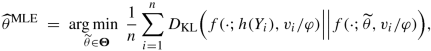
by finding an optimal parameter \(\widehat {\theta }^{\text{MLE}}\) somewhere ‘in the middle’ of the observation \(\widehat {\theta }_1^{\text{MLE}} = h(Y_1),\ldots , \widehat {\theta }_n^{\text{MLE}} = h(Y_n)\). This then provides us with, see (2.27),
$$\displaystyle \begin{aligned} \begin{array}{rcl} \prod_{i=1}^n f\left(Y_i; \widetilde{\theta}, v_i/\varphi\right) & =&\displaystyle \left[ \prod_{i=1}^n f\left(Y_i; h\left({Y_i}\right), v_i/\varphi\right)\right] e^{-\frac{1}{2}\sum_{i=1}^n \frac{v_i}{\varphi} {\mathfrak d}\left(Y_i,\kappa'(\widetilde{\theta})\right)} {}\\& \propto&\displaystyle \exp\left\{-\sum_{i=1}^n D_{\text{KL}}\Big(f(\cdot;h(Y_i), v_i/\varphi)\Big|\Big|f(\cdot;{\widetilde{\theta}}, v_i/\varphi)\Big)\right\}, \end{array} \end{aligned} $$(4.11)where ∝ highlights that we drop all terms that do not involve \(\widetilde {\theta }\). This describes the change in joint likelihood by varying the canonical parameter \(\widetilde {\theta }\) over its domain Θ. The first line of (4.11) is in the spirit of minimizing a weighted square loss, but the Gaussian square is replaced by the unit deviance \(\mathfrak {d}\). The second line of (4.11) is in the spirit of information geometry considered in Sect. 2.3, where we try to find a canonical parameter \(\widetilde {\theta }\) that has a small KL divergence to the n individual models being parametrized by h(Y 1), …, h(Y n), thus, the MLE \(\widehat {\theta }^{\text{MLE}}\) provides an optimal balance over the entire set of (independent) observations Y 1, …, Y n w.r.t. the KL divergence.
-
In contrast to the square loss function, the deviance loss function \({\mathfrak D}(\boldsymbol {Y}_n, \mu )\) respects the distributional properties of Y n, see (4.11). That is, if the underlying distribution allows for larger or smaller claims, this fact is appropriately valued in the deviance loss function (supposed that we have chosen the right family of distributions; model uncertainty will be studied in Sect. 11.1, below).
-
Assume we work in the Gaussian model. In this model we have κ(θ) = θ 2∕2 and canonical link h(μ) = μ, see Sect. 2.1.3. This provides unit deviance in the Gaussian case \({\mathfrak d}\left (y, \mu \right ) = (y-\mu )^2\), which is exactly the square loss function for action space \({\mathbb A}=\overline {\mathcal {M}}\). Thus, the square loss function is most appropriate in the Gaussian case.
-
As explained above, we use unit deviances \({\mathfrak d}(y, \mu )\) as a measure of discrepancy. Alternatively, as in the introduction to this section, see (4.6), we can consider Pearson’s χ 2-statistic which corresponds to the weighted square loss function
$$\displaystyle \begin{aligned} X^2(y,\mu) = \frac{(y-\mu)^2}{V(\mu)}, \end{aligned} $$(4.12)where μ↦V (μ) is the variance function of the chosen EDF. Similarly, to the deviance loss function (4.9), we can aggregate these Pearson’s χ 2-statistics X 2(Y i, μ) over all observations Y i in Y n to receive a second overall measure of discrepancy. In the Gaussian case the deviance loss and Pearson’s χ 2-statistic coincide and have a χ 2-distribution, for other distributions asymptotic results are available.
In the non-Gaussian case, (4.12) is not always robust. For instance, if we work in the Poisson model, we have variance function V (μ) = μ. Our examples below will have low claim frequencies which implies that μ will be small. The appearance of a small μ in the denominator of (4.12) will imply that Pearson’s χ 2-statistic is not very robust in small frequency applications, in particular, if we need to estimate this μ from Y n. Therefore, we refrain from using (4.12).

Naturally, in analogy to Theorem 4.1 and derivation (4.6), the above considerations motivate us to consider expected GLs under unit deviances within the EDF. We use the decision rule \(\widehat {\mu }^{\text{MLE}}(\boldsymbol {Y}_n) \in {\mathbb A}=\overline {\mathcal {M}}\) to predict a new observation Y .
The expected deviance GL is defined and given by
the last identity uses independence between Y n and Y , and with estimation risk function
we use steepness of the cumulant function, \({\mathfrak C}=\overline {\mbox{conv}}({\mathfrak T})=\overline {\mathcal {M}}\), and Lemma 2.22 for the strict positivity of the estimation risk function. Thus, for the estimation risk function \(\mathcal {E}\) we replace Y by μ in the unit deviance and the expectation \({\mathbb E}_\theta \) is only over the observations Y n. This looks like a very convincing generalization of the MSEP, however, one needs to ensure that all terms in (4.13) exist.
Theorem 4.7 (Expected Deviance Generalization Loss). Assume that Y
n and Y are independent and belong to the same linear EDF having the same canonical parameter  and having strictly convex and steep cumulant function κ. Choose a predictor \(A:{\mathbb Y} \to {\mathbb A}=\overline {\mathcal {M}}\), Y
n↦A(Y
n) and assume that all expectations in the following formula exist. The expected deviance GL of predictor A to predict Y is given by
and having strictly convex and steep cumulant function κ. Choose a predictor \(A:{\mathbb Y} \to {\mathbb A}=\overline {\mathcal {M}}\), Y
n↦A(Y
n) and assume that all expectations in the following formula exist. The expected deviance GL of predictor A to predict Y is given by
Remarks 4.8.
-
\({\mathbb E}_\theta [{\mathfrak d}(Y, \mu )]\) plays the role of the pure process variance (irreducible risk) of Theorem 4.1. This term does not involve any parameter estimation bias and uncertainty because it is based on the true parameter θ and μ = κ′(θ), respectively. In Sect. 4.1.3, below, we are going to justify the appropriateness of this object as a tool for forecast evaluation. In particular, because the unit deviance is strictly consistent for the mean functional, the true mean μ = μ(θ) minimizes \({\mathbb E}_\theta [{\mathfrak d}(Y, \mu )]\), see (4.28), below.
-
The second term \(\mathcal {E}\left (\mu , A(\boldsymbol {Y}_n) \right )\) measures parameter estimation bias and uncertainty of decision rule A(Y n) versus the true parameter μ = κ′(θ). The first remark is that we can do this for any decision rule A, i.e., we do not necessarily need to consider the MLE. The second remark is that we can no longer get a clear cut differentiation between a bias term and a parameter estimation uncertainty term for deviance loss functions not coming from the Gaussian distribution. We come back to this in Remarks 7.17, below, where we give more characterization to the individual terms of the expected deviance GL.
-
An issue in applying Theorem 4.7 to the MLE decision rule \(A(\boldsymbol {Y}_n)=\widehat {\mu }^{\text{MLE}}(\boldsymbol {Y}_n)\) is that, in general, it does not lead to a finite estimation risk function. For instance, in the Poisson case we have with positive probability \(\widehat {\mu }^{\text{MLE}}(\boldsymbol {Y}_n)=0\), which results in an infinite estimation risk. In order to avoid this, we need to bound away the decision rule form the boundary of \(\mathcal {M}\) and Θ, respectively. In the Poisson case this can be achieved by considering a decision rule \(A(\boldsymbol {Y}_n)=\max \{\widehat {\mu }^{\text{MLE}}(\boldsymbol {Y}_n), \epsilon \}\) for a fixed given 𝜖 ∈ (0, μ = κ′(θ)). This decision rule has a bias which asymptotically vanishes as n →∞. Moreover, consistency and asymptotic normality tells us that this lower bound does not affect prediction for large sample sizes n (with large probability).
-
Similar to (4.3), we can also consider the deviance GL, given Y n. Under independence of Y n and Y we have deviance GL
$$\displaystyle \begin{aligned} \begin{array}{rcl} {\mathbb E}_\theta\left[\left.{\mathfrak d}\left(Y, A(\boldsymbol{Y}_n)\right)\right|\boldsymbol{Y}_n\right] & =&\displaystyle {\mathbb E}_\theta\left[\left.{\mathfrak d}\left(Y, \mu\right)\right| \boldsymbol{Y}_n\right] + \mathfrak{d}(\mu, A(\boldsymbol{Y}_n)) {}\\& \ge&\displaystyle {\mathbb E}_\theta\left[{\mathfrak d}\left(Y, \mu\right)\right]. \end{array} \end{aligned} $$(4.15)Thus, here we directly compare A(Y n) to the true parameter μ.
Example 4.9 (Estimation Risk Function in the Gaussian Case). We consider the Gaussian case with cumulant function κ(θ) = θ 2∕2 and canonical link h(μ) = μ. The estimation risk function is in the Gaussian case for a square integrable predictor A(Y n) given by
These are exactly the squared bias and the estimation variance, see (4.1). Thus, in the Gaussian case, the MSEP and the expected deviance GL coincide. Moreover, adding a deterministic bias \(c \in {\mathbb R}\) to A(Y n) increases the estimation risk function, supposed that A(Y n) is unbiased for μ. We emphasize the latter as this is an important property to have, and we refer to the next Example 4.10 for an example where this property fails to hold. \(\blacksquare \)
Example 4.10 (Estimation Risk Function in the Poisson Case). We consider the Poisson case with cumulant function κ(θ) = e θ and canonical link h(μ) = logμ. The estimation risk function is given by (subject to existence)
Assume that decision rule A(Y n) is non-deterministic and unbiased for μ. Using Jensen’s inequality these assumptions imply for the estimation risk function
We now add a small deterministic bias \(c\in {\mathbb R}\) to the unbiased estimator A(Y n) for μ. This gives us estimation risk function, see (4.16) and subject to existence,
Consider the derivative w.r.t. bias c in 0, we use Jensen’s inequality on the last line,
Thus, the estimation risk becomes smaller if we add a small bias to the (non-deterministic) unbiased predictor A(Y n). This issue has been raised in Denuit et al. [97]. Of course, this is a very unfavorable property, and it is rather different from the Gaussian case in Example 4.9. It is essentially driven by the fact that parameter estimation is based on a finite sample, which implies a strict inequality in (4.17) for the finite sample estimate A(Y n). A conclusion of this example is that if we use expected deviance GLs for forecast evaluation we need to insist on having unbiased predictors. This will become especially important for more complex regression models, see Sect. 7.4.2, below.
More generally, one can prove this result of a smaller estimation risk function for a small positive bias for any EDF member with power variance function V (μ) = μ p with p ≥ 1, see also (4.18) below. The proof uses the Fortuin–Kasteleyn–Ginibre (FKG) inequality [133] providing \({\mathbb E}_\theta [A(\boldsymbol {Y}_n)^{1-p}]< {\mathbb E}_\theta [A(\boldsymbol {Y}_n)] {\mathbb E}_\theta [A(\boldsymbol {Y}_n)^{-p}] =\mu {\mathbb E}_\theta [A(\boldsymbol {Y}_n)^{-p}]\) to receive (4.17) for power variance parameters p ≥ 1. \(\blacksquare \)
Remarks 4.11 (Conclusion from Examples 4.9 and 4.10 and a Further Remark).
-
Working with expected deviance GLs for evaluating forecasts requires some care because a bigger bias in the (finite sample) estimate A(Y n) may provide a smaller estimation risk function \(\mathcal {E}(\mu , A(\boldsymbol {Y}_n))\). For this reason, we typically insist on having unbiased predictors/forecasts. The latter is also an important requirement in financial applications to guarantee that the overall price is set to the right level, we refer to the balance property in Corollary 3.19 and to Sect. 7.4.2, below.
-
In Theorems 4.1 and 4.7 we use independence between the predictor A(Y n) and the random variable Y to receive the split of the expected deviance GL into irreducible risk and estimation risk function. In regression models, this independence between the predictor A(Y n) and the random variable Y may no longer hold. In that case we will still work with the expected deviance GL \({\mathbb E}_\theta [{\mathfrak d}(Y, A(\boldsymbol {Y}_n))]\), but a clear split between estimation and forecasting will no longer be possible, see Sect. 4.2, below.
The next example gives the most important unit deviances in actuarial modeling.
Example 4.12 (Unit Deviances). We give the most prominent examples of unit deviances within the single-parameter linear EDF. We recall unit deviance (2.25)
In Sect. 2.2 we have met the examples given in Table 4.1.
If we focus on Tweedie’s distributions having power variance functions V (μ) = μ p, see Table 2.1, we get a unified expression for the unit deviances for p ∈{0}∪ (1, 2) ∪ (2, ∞)
For the remaining power variance cases we have: p = 1 corresponds to the Poisson case, p = 2 gives the gamma case, the cases p < 0 do not have a steep cumulant function, and, moreover, there are no EDF models for p ∈ (0, 1), see Theorem 2.18.
The unit deviance in the Bernoulli case is also called binary cross-entropy. This binary cross-entropy has a categorical generalization, called multi-class cross-entropy. Assume we have a categorical EF with levels {1, …, k + 1} and corresponding probabilities p
1, …, p
k+1 ∈ (0, 1) summing up to 1, see Sect. 2.1.4. We denote by  the indicator variable that shows which level the categorical random variable Y takes; Y is called one-hot encoding of the categorical random variable Y . Assume y is a realization of Y and set
  . The categorical (multi-class) cross-entropy loss function is given by
This cross-entropy is closely related to the KL divergence between two categorical distributions p and q on {1, …, k + 1}. The KL divergence from p to q is given by
If we replace the true (but unknown) distribution q by observation Y = y we receive unit deviance (4.19) (scaled by 2), and the MLE is obtained by minimizing this KL divergence, see also Example 3.10. \(\blacksquare \)
Outlook 4.13. In the regression modeling, below, each response Y i will have its own mean parameter μ i = μ(β, x i) which will be a function of its covariate information x i, and β denotes a regression parameter to be estimated with MLE. In that case, we modify the deviance loss function (4.9) to
and the MLE of β can be found by solving

If Y is a new response with covariate information x and following the same EDF as Y n, we will evaluate the corresponding expected scaled deviance GL given by
where \({\mathbb E}_{\boldsymbol {\beta }}\) is the expectation under the true regression parameter β for Y n and Y . This will be discussed in Sect. 5.1.7, below. If we interpret (Y, x, v) as a random vector describing a randomly selected insurance policy from our portfolio, and being independent of Y n (and the corresponding covariate information x i, 1 ≤ i ≤ n), then \(\widehat {\boldsymbol {\beta }}^{\text{MLE}}\) will be independent of (Y, x, v). Nevertheless, the predictor \(\mu (\widehat {\boldsymbol {\beta }}^{\text{MLE}}, \boldsymbol {x})\) will introduce dependence between the chosen decision rule and Y through x, and we no longer receive the split of the expected deviance GL as stated in Theorem 4.7, for a related discussion we also refer to Remarks 7.17, below.
If we interpret (Y, x, v) as a randomly selected insurance policy, then the expected GL (4.22) is evaluated under the joint (portfolio) distribution of (Y, x, v), and the deviance loss \({\mathfrak D}(\boldsymbol {Y}_n, \widehat {\boldsymbol {\beta }}^{\text{MLE}})\) is an (in-sample) empirical version of (4.22). \(\blacksquare \)
4.1.3 A Decision-Theoretic Approach to Forecast Evaluation
We present an excursion to a decision-theoretic approach to forecast evaluation. This excursion gives the theoretical foundation to the unit deviance considerations from above. This section follows Gneiting [162], Krüger–Ziegel [227] and Denuit et al. [97], and we refrain from giving complete proofs in this section. Forecast evaluation should involve consistent loss/scoring functions and proper scoring rules to encourage the forecaster to make careful assessments and honest forecasts. Consistent loss functions are also a necessary tool to receive consistency of M-estimators, we refer to Remarks 3.26.
4.1.3.1 Consistency and Proper Scoring Rules
Denote by \({\mathfrak C} \subseteq {\mathbb R}\) the convex closure of the support of a real-valued random variable Y , and let the action space be \({\mathbb A} = {\mathfrak C}\), see also (3.1). Predictions are evaluated in terms of a loss/scoring function
Remark 4.14. In (4.23) we assume that the loss function L is bounded below by zero. This can be an advantage in applications because it gives a calibration to the loss function. In general, this lower bound is not a necessary condition for forecast evaluation. If we drop this lower bound property, we rather call L (only) a scoring function. For instance, the log-likelihood log(f(y, a)) in (3.27) plays the role of a scoring function.
The forecaster can take the position of minimizing the expected loss to choose her/his action rule. That is, subject to existence, an optimal action w.r.t. L is received by

In this setup the scoring function L(y, a) describes the loss that the forecaster suffers if she/he uses action \(a \in {\mathbb A}\) and observation \(y \in {\mathfrak C}\) materializes. Since we do not want to insist on uniqueness in (4.24) we rather think of set-valued functionals in this section, which may provide solutions to problems like (4.24).Footnote 1
We now reverse the line of arguments, and we start from a general set-valued functional. Denote by \(\mathcal {F}\) the family of distribution functions of interest supported on \({\mathfrak C}\). Consider the set-valued functional
that maps each distribution \(F \in \mathcal {F}\) to a subset \( {\mathfrak A}(F)\) of the action space \({\mathbb A}={\mathfrak C}\), that is, an element of the power set \(\mathcal {P}({\mathbb A})\). The main question that we want to study in this section is the following: can we find a loss function L so that the set-valued functional \({\mathfrak A}\) is obtained by a loss minimization (4.24)? This motivates the following definition. Definition 4.15 (Strict Consistency). The loss function \(L: {\mathfrak C} \times {\mathbb A} \to {\mathbb R}_+\) is consistent for the functional \( {\mathfrak A}: \mathcal {F} \to \mathcal {P}({\mathbb A})\) relative to the class \(\mathcal {F}\) if
for all \(F \in \mathcal {F}\), \(\widehat {a} \in {\mathfrak A}(F)\) and \(a \in {\mathbb A}\). It is strictly consistent if it is consistent and equality in (4.26) implies that \(a \in {\mathfrak A}(F)\).
As stated in Theorem 1 of Gneiting [162], a loss function L is consistent for the functional \( {\mathfrak A}\) relative to the class \(\mathcal {F}\) if and only if, given any \(F \in \mathcal {F}\), every \(\widehat {a} \in {\mathfrak A}(F)\) is an optimal action under L in the sense of (4.24).
We give an example. Assume we start from the functional \(F\mapsto {\mathfrak A}(F)={\mathbb E}_F[Y]\) that maps each distribution F to its expected value. In this case we do not need to consider a set-valued functional because the expected value is a singleton (we assume that \(\mathcal {F}\) only contains distributions with a finite first moment). The question then is whether we can find a loss function L such that this mean can be received by a minimization (4.24). This question is answered in Theorem 4.19, below.
Next we relate a consistent loss function L to a proper scoring rule. A proper scoring rule is a function \(R:{\mathfrak C} \times \mathcal {F} \to {\mathbb R}\) such that
for all \(F,G \in \mathcal {F}\), supposed that the expectations are well-defined. A scoring rule R analyzes the penalty R(y, G) if the forecaster works with a distribution G and an observation y of Y ∼ F materializes. Proper scoring rules have been promoted in Gneiting–Raftery [163] and Gneiting [162]. They are important because they encourage the forecaster to make honest forecasts, i.e., it gives the forecaster the incentive to minimize the expected score by following his true belief about the true distribution, because only this minimizes the expected penalty in (4.27).
Theorem 4.16 (Gneiting [162, Theorem 3]). Assume that L is a consistent loss function for the functional \( {\mathfrak A}\) relative to the class \(\mathcal {F}\). For each \(F \in \mathcal {F}\), let \(a_F \in {\mathfrak A}(F)\). The scoring rule
is a proper scoring rule.
Example 4.17. Consider the unit deviance \({\mathfrak d}\left (\cdot , \cdot \right ) : {\mathfrak C}\times \mathcal {M} \to {\mathbb R}_+\) for a given EDF  with cumulant function κ. Lemma 2.22 says that under suitable assumptions this unit deviance \({\mathfrak d}\left (y, \mu \right )\) is zero if and only if y = μ. We consider the mean functional on \(\mathcal {F}\)
where μ = μ(θ) = κ′(θ) is the mean of the chosen EDF. Choosing the unit deviance as loss function we receive for any action \(a \in {\mathbb A}\), see (4.13),
This is minimized for a = μ and it proves that the unit deviance is strictly consistent for the mean functional \( {\mathfrak A}:F_\theta \mapsto {\mathfrak A}(F_\theta )=\mu (\theta )\) relative to the chosen EDF  . Using Theorem 4.16, the scoring rule
is a strictly proper scoring rule, that is,
for any \(\widetilde {\theta }\neq \theta \). We conclude from this small example that the unit deviance is a strictly consistent loss function for the mean functional on the chosen EDF, and this provides us with a strictly proper scoring rule. \(\blacksquare \)
In the above Example 4.17 we have chosen the mean functional
within a given EDF  . We have seen that
-
the unit deviance \({\mathfrak d}(\cdot ,\cdot )\) is a strictly consistent loss function for the mean functional \({\mathfrak A}\) relative to the EDF \(\mathcal {F}\);
-
the function \((y,F_\theta )\mapsto R(y,F_\theta )={\mathfrak d}(y,\mu (\theta ))\) is a strictly proper scoring rule for the EDF \(\mathcal {F}\), i.e.,
$$\displaystyle \begin{aligned} {\mathbb E}_\theta \left[ {\mathfrak d}(Y, \mu(\theta)) \right] ~< ~ {\mathbb E}_\theta \left[ {\mathfrak d}(Y, \mu(\widetilde{\theta})) \right], \end{aligned}$$for any \(\widetilde {\theta }\neq \theta \).
The consideration of the mean functional \(F\mapsto {\mathfrak A}(F)={\mathbb E}_F[Y]\) in Example 4.17 is motivated by the fact that we typically forecast random variables by their means. However, more generally, we may ask the question for which functionals \( {\mathfrak A}:\mathcal {F} \to \mathcal {P}({\mathbb A})\), relative to a given set of distributions \(\mathcal {F}\), there exists a loss function L that is strictly consistent.
Definition 4.18 (Elicitable). The functional \( {\mathfrak A}\) is elicitable relative to a given set of distributions \(\mathcal {F}\) if there exists a loss function L that is strictly consistent for \( {\mathfrak A}\) and \(\mathcal {F}\).
Above we have seen that the mean functional is elicitable relative to the EDF using the unit deviance loss; expected values relative to \(\mathcal {F}\) with finite second moments are also elicitable using the square loss function. Savage [327] more generally identifies the Bregman divergences as being the only consistent scoring functions for the mean functional; recall that the unit deviance is a special case of a Bregman divergence, see (2.29). We are going to state the corresponding result.
For a general loss function L we make the following (standard) assumptions:
- (L0):
-
L(y, a) ≥ 0 and we have an equality if and only if y = a;
- (L1):
-
L(y, a) is measurable in y and continuous in a;
- (L2):
-
the partial derivative ∂L(y, a)∕∂a exists and is continuous in a whenever a ≠ y.
This then allows us to cite the following theorem. Theorem 4.19 (Gneiting [162, Theorem 7]). Let \(\mathcal {F}\) be the class of distributions on an interval \({\mathfrak C} \subseteq {\mathbb R}\) having finite first moments.
-
Assume the loss function \(L:{\mathfrak C}\times {\mathbb A} \to {\mathbb R}\) satisfies (L0)–(L2) for interval \({\mathfrak C}={\mathbb A} \subseteq {\mathbb R}\). L is consistent for the mean functional relative to the class \(\mathcal {F}\) of compactly supported distributions on \({\mathfrak C}\) if and only if the loss function L is of Bregman divergence form
$$\displaystyle \begin{aligned} D_\psi(y,a) =\psi (y)-\psi(a) -\psi'(a)(y-a), \end{aligned}$$for a convex function ψ with (sub-)gradient ψ′ on \({\mathfrak C}\).
-
If ψ is strictly convex on \({\mathfrak C}\), then the Bregman divergence D ψ is strictly consistent for the mean functional relative to the class \(\mathcal {F}\) on \({\mathfrak C}\) for which both \({\mathbb E}_F[Y]\) and \({\mathbb E}_F[\psi (Y)]\) exist and are finite.
Theorem 4.19 tells us that Bregman divergences are the only consistent loss functions for the mean functional (under some additional assumptions). Consider the specific choice ψ(a) = a 2∕2 which is a strictly convex function. For this choice, the Bregman divergence is the square loss function D ψ(y, a) = (y − a)2∕2, which is strictly consistent for the mean functional relative to the class \(\mathcal {F}\subset L^2({\mathbb P})\). We remark that also quantiles are elicitable, the corresponding result is going to be stated in Theorem 5.33, below.
The second bullet point of Theorem 4.19 immediately implies that the unit deviance \({\mathfrak d}(\cdot ,\cdot )\) is a strictly consistent loss function for the mean functional within the chosen EDF, see also (2.29) and Example 4.17. In particular, for 

Explicit evaluation of (4.28) requires that the true distribution F θ of Y is known. Since, typically, this is not the case, we need to evaluate it empirically. Assume that the random variables Y i are independent and F θ distributed, with F θ belonging to the fixed EDF providing the corresponding unit deviance \({\mathfrak d}\). Then, the objective function in (4.28) is approximated by, a.s.,
The convergence statement follows from the strong law of large numbers applied to the i.i.d. random variables (Y i, v i), i ≥ 1, and supposed that the right-hand side of (4.29) exists. Thus, the deviance loss function (4.9) is an empirical version of the expected deviance loss function, and this approach is successful if we can exchange the ‘argmin’ operator of (4.28) and the limit n →∞ in (4.29). This closes the circle and brings us back to the M-estimator considered in Remarks 3.26 and 3.29, and which also links forecast evaluation and M-estimation.
4.1.3.2 Forecast Dominance
A consequence of Theorem 4.19 is that there are infinitely many strictly consistent loss functions for the mean functional, and, in principle, we could choose any of these for forecast evaluation. Choosing the unit deviance \({\mathfrak d}\) that matches the distribution F θ of the observations Y n and Y , respectively, gives us the MLE \(\widehat {\mu }^{\text{MLE}}\), and we have seen that the MLE \(\widehat {\mu }^{\text{MLE}}\) is not only unbiased for μ = κ′(θ), but it also meets the Cramér–Rao information bound. That is, it is UMVU within the data generating model reflected by the true unit deviance \({\mathfrak d}\). This provides us (in the finite sample case) with a natural candidate for \({\mathfrak d}\) in (4.29) and, thus, a canonical proper scoring rule for (out-of-sample) forecast evaluation.
The previous statements have all been done under the assumption that there is no uncertainty about the underlying family of distribution functions that generates Y and Y n, respectively. Uncertainty was limited to the true canonical parameter θ and the true mean μ(θ). This situation changes under model uncertainty. Krüger–Ziegel [227] study the question of having multiple strictly consistent loss functions in the situation where there is no natural candidate choice. Different choices may give different rankings to different (finite sample) predictors. Assume we have two predictors \(\widehat {\mu }_1\) and \(\widehat {\mu }_2\) for a random variable Y . Similarly to the definition of the expected deviance GL, we understand these predictors \(\widehat {\mu }_1\) and \(\widehat {\mu }_2\) as random variables, and we assume that all considered random variables have a finite first moment. Importantly, we do not assume independence between \(\widehat {\mu }_1\), \(\widehat {\mu }_2\) and Y , and in regression models we typically receive dependence between predictors \(\widehat {\mu }\) and random variables Y through the features (covariates) x, see also Outlook 4.13. Following Krüger–Ziegel [227] and Ehm et al. [119] we define forecast dominance as follows. Definition 4.20 (Forecast Dominance). Predictor \(\widehat {\mu }_1\) dominates predictor \(\widehat {\mu }_2\) if
for all Bregman divergences D ψ with (convex) ψ supported on \(\mathfrak {C}\), the latter being the convex closure of the supports of Y , \(\widehat {\mu }_1\) and \(\widehat {\mu }_2\).
If we work with a fixed member of the EDF, e.g., the gamma distribution, then we typically study the corresponding expected deviance GL for forecast evaluation in one single model, see Theorem 4.7 and (4.29). This evaluation may involve model risk in the decision making process, and forecast dominance provides a robust selection criterion.
Krüger–Ziegel [227] build on Theorem 1b and Corollary 1b of Ehm et al. [119] to prove the following theorem (which prevents from considering all convex functions ψ). Theorem 4.21 (Theorem 2.1 of Krüger–Ziegel [227]). Predictor \(\widehat {\mu }_1\) dominates predictor \(\widehat {\mu }_2\) if and only if for all \(\tau \in {\mathfrak C}\)

Denuit et al. [97] argue that in insurance one typically works with Tweedie’s distributions having power variances V (μ) = μ p with power variance parameters p ≥ 1. This motivates the following weaker form of forecast dominance. Definition 4.22 (Tweedie’s Forecast Dominance). Predictor \(\widehat {\mu }_1\) Tweedie-dominates predictor \(\widehat {\mu }_2\) if
for all Tweedie’s unit deviances \(\mathfrak {d}_p\) with power variance parameters p ≥ 1, we refer to (4.18) for p ∈ (1, ∞) ∖{2} and Table 4.1 for the Poisson and gamma cases p ∈{1, 2}.
Recall that Tweedie’s unit deviances \(\mathfrak {d}_p\) are a subclass of Bregman divergences, see (2.29). Define the following function for power variance parameters p ≥ 1
Denuit et al. [97] prove the following proposition. Proposition 4.23 (Proposition 4.1 of Denuit et al. [97]). Predictor \(\widehat {\mu }_1\) Tweedie-dominates predictor \(\widehat {\mu }_2\) if
and

Theorem 4.21 gives necessary and sufficient conditions to have forecast dominance, Proposition 4.23 gives sufficient conditions to have the weaker Tweedie’s forecast dominance. In Theorem 7.15, below, we give another characterization of forecast dominance in terms of convex orders, under the additional assumption that the predictors are so-called auto-calibrated.
4.2 Cross-Validation
This section focuses on estimating the expected deviance GL (4.13) in cases where the canonical parameter θ is not known. Of course, the same concepts apply to the MSEP. In the remainder of this section we scale the unit deviances with v∕φ, to bring them in line with the deviance loss (4.9).
4.2.1 In-Sample and Out-of-Sample Losses
The general aim in predictive modeling is to predict an unobserved random variable Y as good as possible based on past information Y n. Within the EDF, the predictive performance is then evaluated under an empirical version of the expected deviance GL
Here, we no longer assume that Y and A(Y n) are independent, and in the dependent case Theorem 4.7 does not apply. The reason for dropping the independence assumption is that below we consider regression models of a similar type as in Outlook 4.13. The expected deviance GL (4.31) as such is not directly useful because it cannot be calculated if the true canonical parameter θ is not known. Therefore, we are going to explain how it can be estimated empirically.
We start from the expected deviance GL in the EDF applied to the MLE decision rule \(\widehat {\mu }^{\text{MLE}}(\boldsymbol {Y}_n)\). It can be rewritten as
where we use the tower property for conditional expectations. In view of (4.32), there are two things to be done:
-
(1)
For given observations Y n = y n, we need to estimate the deviance GL, see also (4.15),
$$\displaystyle \begin{aligned} {\mathbb E}_\theta\left.\left[\frac{v}{\varphi}{\mathfrak d}\left(Y, \widehat{\mu}^{\text{MLE}}(\boldsymbol{Y}_n)\right) \right| \boldsymbol{Y}_n=\boldsymbol{y}_n\right] = {\mathbb E}_\theta\left.\left[\frac{v}{\varphi}{\mathfrak d}\left(Y, \widehat{\mu}^{\text{MLE}}(\boldsymbol{y}_n)\right) \right| \boldsymbol{Y}_n=\boldsymbol{y}_n\right]. \end{aligned} $$(4.33)This is the part that we are going to solve empirically in the this section. Typically, we assume that Y and Y n are independent, nevertheless, Y and its MLE predictor may still be dependent because we may have a predictor \(\widehat {\mu }^{\text{MLE}}(\boldsymbol {Y}_n)=\widehat {\mu }^{\text{MLE}}(\boldsymbol {Y}_n, \boldsymbol {x})\). That is, this predictor often depends on covariate information x that describes Y , an example is provided in (4.22) of Outlook 4.13 and this is different from (4.15). In that case, the decision rule \(A:{\mathbb Y} \times \mathcal {X} \to {\mathbb A}\) is extended by an additional covariate component \(\boldsymbol {x} \in \mathcal {X}\), we refer to Sect. 5.1.1, where \(\mathcal {X}\) is introduced and discussed.
-
(2)
We have to find a way to generate more observations Y n from P(y n;θ) in order to evaluate the outer integral in (4.32) empirically. One way to do so is the bootstrap method that is going to be discussed in Sect. 4.3, below.
We address the first problem of estimating the deviance GL given in (4.33). We do this under the assumption that Y n and Y are independent. In order to estimate (4.33) we need observations for Y . However, typically, there are no observations available for this random variable because it is only going to be observed in the future. For this reason, one uses past observations for both, model fitting and the GL analysis. In order to perform this analysis in a proper way, the general paradigm is to partition the entire data into two disjoint data sets, a so-called learning data set \(\mathcal {L}=\{Y_1,\ldots , Y_n\}\) and a test data set \(\mathcal {T}=\{Y^\dagger _1,\ldots , Y^\dagger _T\}\). If we assume that all observations in \(\mathcal {L}\cup \mathcal {T}\) are independent, then we receive a suitable observation Y n from the learning data set \(\mathcal {L}\) that can be used for model fitting. The test sample \(\mathcal {T}\) can then play the role of the unobserved random variable Y (by assumption being independent of Y n). Note that \(\mathcal {L}\) is only used for model fitting and \(\mathcal {T}\) is only used for the deviance GL evaluation, see Fig. 4.1.

Partition of entire data into learning data set \(\mathcal {L}\) and test data set \(\mathcal {T}\)
This setup motivates to estimate the mean parameter μ with MLE \(\widehat {\mu }^{\text{MLE}}_{\mathcal {L}}=\widehat {\mu }^{\text{MLE}}(\boldsymbol {Y}_n)\) from the learning data \(\mathcal {L}\) and Y n, respectively, by minimizing the deviance loss function \(\mu \mapsto {\mathfrak D}(\boldsymbol {Y}_n, \mu )\) on the learning data \(\mathcal {L}\), according to Corollary 4.5. Then we use this predictor \(\widehat {\mu }^{\text{MLE}}_{\mathcal {L}}\) to empirically evaluate the conditional expectation in (4.33) on \(\mathcal {T}\). The perception used is that we (in-sample) learn a model on \(\mathcal {L}\) and we out-of-sample test this model on \(\mathcal {T}\) to see how it generalizes to unobserved variables \(Y^\dagger _t\), 1 ≤ t ≤ T, that are of a similar nature as Y . Definition 4.24 (In-Sample and Out-of-Sample Losses). The in-sample deviance loss on the learning data \(\mathcal {L}=\{Y_1,\ldots , Y_n\}\) is given by
with MLE \(\widehat {\mu }^{\text{MLE}}_{\mathcal {L}}=\widehat {\mu }^{\text{MLE}}(\boldsymbol {Y}_n)\) on \(\mathcal {L}\).
The out-of-sample deviance loss on the test data \(\mathcal {T}=\{Y^\dagger _1,\ldots , Y^\dagger _T\}\) of predictor \(\widehat {\mu }^{\text{MLE}}_{\mathcal {L}}\) is
where the sum runs over the test sample \(\mathcal {T}\) having exposures \(v^\dagger _1,\ldots , v^\dagger _T>0\).
For MLE we minimize the objective function (4.9), therefore, the in-sample deviance loss \({\mathfrak D}(\mathcal {L}, \widehat {\mu }^{\text{MLE}}_{\mathcal {L}}) ={\mathfrak D}(\boldsymbol {Y}_n, \widehat {\mu }^{\text{MLE}}(\boldsymbol {Y}_n))\) exactly corresponds to the minimal deviance loss (4.9) achieved on the learning data \(\mathcal {L}\), i.e., when using MLE \(\widehat {\mu }^{\text{MLE}}_{\mathcal {L}}=\widehat {\mu }^{\text{MLE}}(\boldsymbol {Y}_n)\). We call this in-sample because the same data \(\mathcal {L}\) is used for parameter estimation and deviance loss calculation. Typically, this loss is biased because it uses the optimal (in-sample) parameter estimate, we also refer to Sect. 4.2.3, below.
The out-of-sample loss \({\mathfrak D}(\mathcal {T}, \widehat {\mu }^{\text{MLE}}_{\mathcal {L}})\) then empirically estimates the inner expectation in (4.32). This is a proper out-of-sample analysis because the test data \(\mathcal {T}\) is disjoint from the learning data \(\mathcal {L}\) on which the decision rule \(\widehat {\mu }^{\text{MLE}}_{\mathcal {L}}\) has been trained. Note that this out-of-sample figure reflects (4.33) in the following sense. We have a portfolio of risks \((Y^\dagger _t,v^\dagger _t)\), 1 ≤ t ≤ T, and (4.33) does not only reflect the calculation of the deviance GL of a given risk, but also the random selection of a risk from the portfolio. In this sense, (4.33) is an average over a given portfolio whose description is also included in the probability \({\mathbb P}_\theta \).
Summary 4.25. Definition 4.24 gives the general principle in predictive modeling according to which model learning and the generalization analysis are done. Namely, based on two disjoint and independent data sets \(\mathcal {L}\) and \(\mathcal {T}\), we perform model calibration on \(\mathcal {L}\), and we analyze (conditional) GLs (using out-of-sample losses) on \(\mathcal {T}\), respectively. For this concept to be useful, the learning data \(\mathcal {L}\) and the test data \(\mathcal {T}\) have to be sufficiently similar, i.e., ideally coming from the same model.
This approach does not estimate the outer expectation in the expected deviance GL (4.32), i.e., it is only an estimate for the deviance GL, given Y n, see (4.33).
4.2.2 Cross-Validation Techniques
In many applications one is not in the comfortable situation of having two sufficiently large data sets \(\mathcal {L}\) and \(\mathcal {T}\) available to support model learning and an out-of-sample generalization analysis. That is, we are usually equipped with only one data set of average size, let us call it \(\mathcal {D}\). In order to calculate the objects in Definition 4.24 we could partition this data set (at random) into two data sets and then calculate in-sample and out-of-sample deviance losses on this partition. The disadvantage of this approach is that it is an inefficient use of information if only little data is available. In that case we require (almost) all data for learning. However, we still need a sufficiently large share of data for testing, to receive reliable deviance GL estimates for (4.33). The classical approach in this situation is to use cross-validation for estimating out-of-sample losses. The concept works as follows:
-
1.
Perform model learning and in-sample loss calculation \({\mathfrak D}(\mathcal {L}, \widehat {\mu }^{\text{MLE}}_{\mathcal {L}}) \) on all available data \(\mathcal {L}=\mathcal {D}\), i.e., this part is not affected by selecting test data \(\mathcal {T}\) and it is not touched by cross-validation.
-
2.
For out-of-sample deviance loss calculation use the data \(\mathcal {D}\) iteratively in an efficient way such that part of the data is used for model learning and the other part for the out-of-sample generalization analysis. This second step is (only) done for estimating the deviance GL of the model learned on all data. I.e. for prediction we work with MLE \(\widehat {\mu }^{\text{MLE}}_{\mathcal {L}=\mathcal {D}}\), but the out-of-sample deviance loss is estimated using this data in a different way.
The three most commonly used methods are leave-one-out, K-fold and stratified K-fold cross-validation. We briefly describe these three cross-validation methods.
4.2.2.1 Leave-One-Out Cross-Validation
Denote all available data by \(\mathcal {D} =\{Y_1,\ldots , Y_{n}\}\), and assume independence between the components. For leave-one-out (loo) cross-validation we select 1 ≤ i ≤ n and define the partition \(\mathcal {L}_{(-i)} = \mathcal {D}\setminus \{Y_i\}\) for the learning data and \(\mathcal {T}_i=\{Y_i\}\) for the test data. Based on the learning data \(\mathcal {L}_{(-i)}\) we calculate the MLE

which is based on all data except observation Y i. This observation is now used to do an out-of-sample analysis, and averaging this over all 1 ≤ i ≤ n we receive the leave-one-out cross-validation loss
where \( {\mathfrak D}(\mathcal {T}_i, \widehat {\mu }^{(-i)})\) is the (out-of-sample) cross-validation loss on \(\mathcal {T}_i=\{Y_i\}\) using the predictor \(\widehat {\mu }^{(-i)}\). This leave-one-out cross-validation loss \(\widehat {\mathfrak D}^{\text{loo}}\) is now used as estimate for the out-of-sample deviance loss \({\mathfrak D}(\mathcal {T}, \widehat {\mu }^{\text{MLE}}_{\mathcal {L}})\). Leave-one-out cross-validation uses all data \(\mathcal {D}\) for learning and testing, namely, the data \(\mathcal {D}\) is partitioned into a learning set \(\mathcal {L}_{(-i)}\) for (partial) learning and a test set \(\mathcal {T}_i=\{Y_i\}\) for an out-of-sample generalization analysis. This is done for all instances 1 ≤ i ≤ n, and the out-of-sample loss is estimated by the resulting average cross-validation loss. This averaging allows us to not only understand (4.34) as a conditional out-of-sample loss in the spirit of Definition 4.24. The outer empirical average in (4.34) also makes it suitable for an expected deviance GL estimate according to (4.32).
The variance of this empirical deviance GL is given by (subject to existence)
These covariances use exactly the same observations on \(\mathcal {D}\setminus \{Y_i,Y_j\}\), therefore, there are strong correlations between the estimators \(\widehat {\mu }^{(-i)}\) and \(\widehat {\mu }^{(-j)}\). In addition, the leave-one-out cross-validation is often computationally not feasible because it requires fitting the model n times, which in the situation of complex models and of large insurance portfolios can be too demanding. We come back to this in Sect. 5.6 where we provide the generalized cross-validation (GCV) loss approximation within generalized linear models (GLMs).
4.2.2.2 K-Fold Cross-Validation
Choose a fixed integer K ≥ 2 and partition the entire data \(\mathcal {D}\) at random into K disjoint subsets (called folds) \(\mathcal {L}_1,\ldots , \mathcal {L}_K\) of approximately the same size. The learning data for fixed 1 ≤ k ≤ K is then defined by \(\mathcal {L}_{[-k]} = \mathcal {D}\setminus \mathcal {L}_k\) and the test data by \(\mathcal {T}_k=\mathcal {L}_k\), see Fig. 4.2. Based on learning data \(\mathcal {L}_{[-k]}\) we calculate the MLE

which is based on all data except \(\mathcal {T}_k\).

Partitions of K-fold cross-validation for K = 5
These observations are now used to do an (out-of-sample) cross-validation analysis, and averaging this over all 1 ≤ k ≤ K we receive the K-fold cross-validation (CV) loss.
The last step is an approximation because not all \(\mathcal {T}_k\) may have exactly the same sample size if n is not a multiple of K. We can understand (4.35) not only as a conditional out-of-sample loss estimate in the spirit of Definition 4.24. The outer empirical average in (4.35) also makes it suitable for an expected deviance GL estimate according to (4.32). The variance of this empirical deviance GL is given by (subject to existence)
Typically, in applications, one uses K-fold cross-validation with K = 10.
4.2.2.3 Stratified K-Fold Cross-Validation
A disadvantage of the above K-fold cross-validation is that it may happen that there are two outliers in the data, and there is a positive probability that these two outliers belong to the same subset \(\mathcal {L}_k\). This may substantially distort K-fold cross-validation because in that case the subsets \(\mathcal {L}_k\), 1 ≤ k ≤ K, are of different quality. Stratified K-fold cross-validation aims at distributing outliers more equally across the partition. Order the observations Y i, 1 ≤ i ≤ n, as follows
For stratified K-fold cross-validation, we randomly distribute (partition) the K biggest claims Y (1), …, Y (K) to the subsets \(\mathcal {L}_k\), 1 ≤ k ≤ K, then we randomly partition the next K biggest claims Y (K+1), …, Y (2K) to the subsets \(\mathcal {L}_k\), 1 ≤ k ≤ K, and so forth. This implies, e.g., that the two biggest claims cannot fall into the same set \(\mathcal {L}_k\). This stratified partition \(\mathcal {L}_k\), 1 ≤ k ≤ K, is then used for K-fold cross-validation.
Summary 4.26 (Cross-Validation).
-
A model is calibrated on the learning data set \(\mathcal {L}\) by minimizing the in-sample deviance loss \({\mathfrak D}(\mathcal {L}, \mu )\) in μ. This provides MLE \(\widehat {\mu }^{\text{MLE}}_{\mathcal {L}}\).
-
The quality of this model is assessed on test data \(\mathcal {T}\) being disjoint of \(\mathcal {L}\) considering the corresponding out-of-sample deviance loss \({\mathfrak D}(\mathcal {T}, \widehat {\mu }^{\text{MLE}}_{\mathcal {L}}) \).
-
If there is no test data set \(\mathcal {T}\) available we perform (stratified) K-fold cross-validation. This provides the (stratified) K-fold cross-validation loss \(\widehat {\mathfrak D}^{\text{CV}}\) which is an estimate for the out-of-sample deviance loss and for the expected deviance GL (4.32).
Example 4.27 (Out-of-Sample Deviance Loss Estimation). We consider a claim counts example using the Poisson EDF model. The claim counts N
i and exposures v
i > 0 used come from the French motor insurance data given in Listing 13.2 of Chap. 13.1. We model the claim frequencies Y
i = N
i∕v
i with the Poisson EDF model having cumulant function \(\kappa (\theta )=\exp \{\theta \}\) and dispersion parameter φ = 1 for all 1 ≤ i ≤ n. The expected frequency is given by \(\mu ={\mathbb E}_\theta [Y_i] =\kappa '(\theta )\). Moreover, we assume that all claim counts N
i, 1 ≤ i ≤ n, are independent. This provides us with the Poisson deviance loss function for observations  , see Example 4.12,
where, for Y i = 0, we set \({\mathfrak d}(Y_i=0,\mu )=2\mu \). Minimizing the Poisson deviance loss function \({\mathfrak D}(\boldsymbol {Y}_n, \mu )\) in μ gives us the MLE for μ and θ = h(μ), respectively. It is given by, see (3.24),
for learning data set \(\mathcal {L}=\{Y_1,\ldots , Y_n\}\). This provides us with an in-sample Poisson deviance loss of \({\mathfrak D}(\boldsymbol {Y}_n, \widehat {\mu }_{\mathcal {L}}^{\text{MLE}}) ={\mathfrak D}(\mathcal {L}, \widehat {\mu }_{\mathcal {L}}^{\text{MLE}})=25.213 \cdot 10^{-2}\).
Since we do not have test data \(\mathcal {T}\), we explore tenfold cross-validation. We therefore partition the entire data at random into K = 10 disjoint sets \(\mathcal {L}_1,\ldots , \mathcal {L}_{10}\), and compute the tenfold cross-validation loss as described in (4.35). This gives us \(\widehat {\mathfrak D}^{\text{CV}}=25.213 \cdot 10^{-2}\), thus, we receive the same value as for the in-sample loss which says that we do not have in-sample over-fitting, here. This is not surprising in the homogeneous model \(\lambda ={\mathbb E}_\theta [Y_i]\). We can also quantify the uncertainty in this estimate by the corresponding empirical standard deviation for \(\mathcal {T}_k=\mathcal {L}_k\)

This says that there is quite some fluctuation in the data because uncertainty in estimate \(\widehat {\mathfrak D}^{\text{CV}}=25.213 \cdot 10^{-2}\) is roughly 1%. This finishes this example, and we will come back to it in Sect. 5.2.4, below. \(\blacksquare \)
4.2.3 Akaike’s Information Criterion
The out-of-sample analysis in terms of GLs and cross-validation evaluates the predictive performance on unseen data. Another way of model selection is to study in-sample losses instead, but penalize model complexity. Akaike’s information criterion (AIC), see Akaike [5], is the most popular tool that follows such a model selection methodology. AIC is based on a set of assumptions which should be fulfilled to apply, this is going to be discussed in this section; we therefore follow the lecture notes of Künsch [229].
Assume we have independent random variables Y i from some (unknown) density f. Assume we have two candidate models with densities h θ and g 𝜗 from which we would like to select the preferred one for the given data Y n = (Y 1, …, Y n). The two unknown parameters in these densities h θ and g 𝜗 are called θ and 𝜗, respectively. We neither assume that one of the two models h θ and g 𝜗 contains the true model f, nor that the two models are nested. That is, f, h θ and g 𝜗 are quite general densities w.r.t. a given σ-finite measure ν.
Assume that both models under consideration have a unique MLE \(\widehat {\theta }^{\text{MLE}}=\widehat {\theta }^{\text{MLE}}(\boldsymbol {Y}_n)\) and \(\widehat {\vartheta }^{\text{MLE}}=\widehat {\vartheta }^{\text{MLE}}(\boldsymbol {Y}_n)\) which is based on the same observations Y n. AIC [5] says that model \(h_{\widehat {\theta }^{\text{MLE}}}\) should be preferred over model \(g_{\widehat {\vartheta }^{\text{MLE}}}\) if
where dim(⋅) denotes the dimension of the corresponding parameter. Thus, we compute the log-likelihoods of the data Y n in the corresponding MLEs \(\widehat {\theta }^{\text{MLE}}\) and \(\widehat {\vartheta }^{\text{MLE}}\), and we penalize the resulting values with the number of parameters to correct for model complexity. We give some remarks.
Remarks 4.28.
-
AIC is neither an in-sample loss nor an out-of-sample loss to measure generalization accuracy, but it considers penalized log-likelihoods. Under certain assumptions one can prove that asymptotically minimizing AICs is equivalent to minimizing leave-one-out cross-validation mean squared errors.
-
The two penalized log-likelihoods have to be evaluated on the same data Y n and they need to consider the MLEs \(\widehat {\theta }^{\text{MLE}}\) and \(\widehat {\vartheta }^{\text{MLE}}\) because the justification of AIC is based on the asymptotic normality of MLEs, otherwise there is no mathematical justification why (4.37) should be a reasonable model selection tool.
-
AIC does not require (but allows for) nested models h θ and g 𝜗 nor need they be Gaussian, it is only based on asymptotic normality. We give a heuristic argument below.
-
Evaluation of (4.37) involves all terms of the log-likelihoods, also those that do not depend on the parameters θ and 𝜗.
-
Both models should consider the data Y n in the same units, i.e., AIC does not apply if h θ is a density for Y i and g 𝜗 is a density for cY i. In that case, one has to perform a transformation of variables to ensure that both densities consider the data in the same units. We briefly highlight this by considering a Gaussian example. We choose i.i.d. observations \(Y_i \sim \mathcal {N}(\theta , \sigma ^2)\) for known variance σ 2 > 0. Choose c > 0, we have \(cY_i \sim \mathcal {N}(\vartheta =c\theta , c^2\sigma ^2)\). We obtain MLE \(\widehat {\theta }^{\text{MLE}}=\sum _{i=1}^n Y_i/n\) and log-likelihood in MLE \(\widehat {\theta }^{\text{MLE}}\)
$$\displaystyle \begin{aligned} \sum_{i=1}^n {\mbox{log}} \left(h_{\widehat{\theta}^{\text{MLE}}}(Y_i)\right) = -\frac{n}{2} {\mbox{log}}(2\pi \sigma^2) - \sum_{i=1}^n \frac{1}{2\sigma^2} \left(Y_i -\widehat{\theta}^{\text{MLE}} \right)^2. \end{aligned}$$On the transformed scale we have MLE \(\widehat {\vartheta }^{\text{MLE}}=\sum _{i=1}^n c Y_i/n =c \widehat {\theta }^{\text{MLE}}\) and log-likelihood in MLE \(\widehat {\vartheta }^{\text{MLE}}\)
$$\displaystyle \begin{aligned} \sum_{i=1}^n {\mbox{log}} \left(g_{\widehat{\vartheta}^{\text{MLE}}}(c Y_i)\right) = -\frac{n}{2} {\mbox{log}}(2\pi c^2\sigma^2) - \sum_{i=1}^n \frac{1}{2 c^2\sigma^2} \left(c Y_i -c\widehat{\theta}^{\text{MLE}}\right)^2. \end{aligned}$$Thus, find that the two log-likelihoods differ by − nlog(c), but we consider the same model only under different measurement units of the data. The same applies when we work, e.g., with a log-normal model or logged data in a Gaussian model.
We give a heuristic justification of AIC. In Example 3.10 we have seen that the MLE is obtained by minimizing the KL divergence from h θ to the empirical distribution \(\widehat {f}_n\) of Y n. This motivates to use the KL divergence also for comparing the MLE estimated models to the true model, i.e., we consider the difference (supposed the densities are defined on the same domain)

If this difference is negative, model \(h_{\widehat {\theta }^{\text{MLE}}}\) should be preferred over model \(g_{\widehat {\vartheta }^{\text{MLE}}}\) because it is closer to the true model f w.r.t. the KL divergence. Thus, we need to calculate the two integrals in (4.38). Since the true density f is not known, these two integrals need to be estimated.
As a first idea we estimate the integrals on the right-hand side empirically using the observations Y n, say, the first integral is estimated by
However, this will lead to a biased estimate because the MLE \(\widehat {\vartheta }^{\text{MLE}}\) exactly maximizes this empirical estimate (as a function of 𝜗). The integrals in (4.38), on the other hand, can be interpreted as an out-of-sample calculation between independent random variables Y
n (used for MLE) and Y ∼ fdν used in the integral. The bias results from the fact that in the empirical estimate the independence gets lost. Therefore, we need to correct this estimate for the bias in order to obtain a reasonable estimate for the difference of the KL divergences. Under the following assumptions this bias correction is asymptotically given by −dim(𝜗)∕n: (1)  is asymptotically normally distributed \(\mathcal {N}(0, \Sigma (\vartheta _0)^{-1})\) as n →∞, where 𝜗
0 is the parameter that minimizes the KL divergence from g
𝜗 to f; we also refer to Remarks 3.26. (2) The true f is sufficiently close to \(g_{\vartheta _0}\) such that the \({\mathbb E}_f\)-covariance matrix of the score \(\nabla _{\vartheta }{\mbox{log}} g_{\vartheta _0}\) is close to the negative \({\mathbb E}_f\)-expected Hessian \(\nabla _{\vartheta }^2{\mbox{log}} g_{\vartheta _0}\); see also (3.36) and Sect. 11.1.4, below. In that case, Σ(𝜗
0) approximately corresponds to Fisher’s information matrix \(\mathcal {I}_1(\vartheta _0)\) and AIC is justified.
is asymptotically normally distributed \(\mathcal {N}(0, \Sigma (\vartheta _0)^{-1})\) as n →∞, where 𝜗
0 is the parameter that minimizes the KL divergence from g
𝜗 to f; we also refer to Remarks 3.26. (2) The true f is sufficiently close to \(g_{\vartheta _0}\) such that the \({\mathbb E}_f\)-covariance matrix of the score \(\nabla _{\vartheta }{\mbox{log}} g_{\vartheta _0}\) is close to the negative \({\mathbb E}_f\)-expected Hessian \(\nabla _{\vartheta }^2{\mbox{log}} g_{\vartheta _0}\); see also (3.36) and Sect. 11.1.4, below. In that case, Σ(𝜗
0) approximately corresponds to Fisher’s information matrix \(\mathcal {I}_1(\vartheta _0)\) and AIC is justified.
This shows that AIC applies if both models are evaluated under the same observations Y n, the models need to use the MLEs, and asymptotic normality needs to hold with limits such that the true model is close to a member of the selected model classes {h θ;θ} and {g 𝜗;𝜗}. We remark that this is not the only set-up under which AIC can be justified, but other set-ups do not essentially differ.
The Bayesian information criterion (BIC) is similar to AIC but in a Bayesian context. The BIC says that model \(h_{\widehat {\theta }^{\text{MLE}}}\) should be preferred over model \(g_{\widehat {\vartheta }^{\text{MLE}}}\) if
where n is the sample size of Y n used for model fitting. The BIC has been derived by Schwarz [331]. Therefore, it is also called Schwarz’ information criterion (SIC).
4.3 Bootstrap
The bootstrap method has been invented by Efron [115] and Efron–Tibshirani [118]. The bootstrap is used to simulate new data from either the empirical distribution \(\widehat {F}_n\) or from an estimated model \(F(\cdot ;\widehat {\theta })\). This allows, for instance, to evaluate the outer expectation in the expected deviance GL (4.32) which requires a data model for Y n. The presentation in this section is based on the lecture notes of Bühlmann–Mächler [59, Chapter 5].
4.3.1 Non-parametric Bootstrap Simulation
Assume we have i.i.d. observations Y 1, …, Y n from an unknown distribution function F(⋅;θ). Based on these observations Y = (Y 1, …, Y n) we choose a decision rule \(A:{\mathbb Y} \to {\mathbb A}=\boldsymbol {\Theta } \subseteq {\mathbb R}\) which provides us with an estimator for θ
Typically, the decision rule A(⋅) is a known function and we would like to determine the distributional properties of parameter estimator (4.39) as a function of the (random) observations Y . E.g., for any measurable set C, we might want to compute

Since, typically, the true data generating distribution Y i ∼ F(⋅;θ) is not known, the distributional properties of \(\widehat {\theta }\) cannot be determined, also not by Monte Carlo simulation. The idea behind bootstrap is to approximate F(⋅;θ). Choose as approximation to F(⋅;θ) the empirical distribution of the i.i.d. observations Y given by, see (3.9),

The Glivenko–Cantelli theorem [64, 159] tells us that the empirical distribution \(\widehat {F}_n\) converges uniformly to F(⋅;θ), a.s., for n →∞, so it should be a good approximation to F(⋅;θ) for large n. The idea now is to simulate from the empirical distribution \(\widehat {F}_n\).
________________________________________________________________________________________________
(Non-parametric) bootstrap algorithm _____________________________________________________________
-
(1)
Repeat for m = 1, …, M
-
(a)
simulate i.i.d. observations \(Y^\ast _1,\ldots , Y^\ast _n\) from \(\widehat {F}_n\) (these are obtained by random drawings with replacements from the observations Y 1, …, Y n; we denote this resampling distribution of \({\boldsymbol {Y}}^\ast =(Y^\ast _1,\ldots , Y^\ast _n)\) by \({\mathbb P}^\ast ={\mathbb P}^\ast _{\boldsymbol {Y}}\));
-
(b)
calculate the estimator \(\widehat {\theta }^{(m\ast )} = A(\boldsymbol {Y}^\ast )\).
-
(a)
-
(2)
Return \(\widehat {\theta }^{(1\ast )}, \ldots , \widehat {\theta }^{(M\ast )}\) and the resulting empirical bootstrap distribution
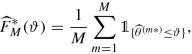
for the estimated distribution of \(\widehat {\theta }\).

_______________________________________________________________
We can use the empirical bootstrap distribution \(\widehat {F}^\ast _M\) as an estimate of the true distribution of \(\widehat {\theta }\), that is, we estimate and approximate

where \({\mathbb P}^\ast _{\boldsymbol {Y}}\) corresponds to the bootstrap distribution of Step (1a) of the above algorithm, and where we set \(\widehat {\theta }^\ast =A(\boldsymbol {Y}^\ast )\). This bootstrap distribution \({{\mathbb P}}_{\boldsymbol {Y}}^\ast \) is empirically approximated by the empirical bootstrap distribution \(\widehat {F}^\ast _M\) for studying \(\widehat {\theta }^\ast \).
Remarks 4.29.
-
The quality of the approximations in (4.41) depend on the richness of the observation Y = (Y 1, …, Y n), because the bootstrap distribution
$$\displaystyle \begin{aligned} {{\mathbb P}}_{\boldsymbol{Y}}^\ast \left[ \widehat{\theta}^\ast \in C \right] ={{\mathbb P}}^\ast_{\boldsymbol{Y}=\boldsymbol{y}} \left[ \widehat{\theta}^\ast \in C \right], \end{aligned}$$depends on the realization y of the data Y from which we generate the bootstrap sample Y ∗. It also depends on M and the explicit random drawings \(Y^\ast _i\) providing the empirical bootstrap distribution \(\widehat {F}^\ast _M\). The latter uncertainty can be controlled since the bootstrap distribution \({\mathbb P}_{\boldsymbol {Y}}^\ast \) corresponds to a multinomial distribution, and the Glivenko–Cantelli theorem [64, 159] applies to \(\widehat {F}^\ast _M\) and \({\mathbb P}_{\boldsymbol {Y}}^\ast \) for M →∞. The former uncertainty inherited from the realization Y = y cannot be diminished because we cannot enrich the observation Y .
-
The empirical bootstrap distribution \(\widehat {F}^\ast _M\) can be used to estimate the mean of the estimator \(\widehat {\theta }\) given in (4.39)
$$\displaystyle \begin{aligned} \widehat{{\mathbb E}}_\theta\left[\widehat{\theta}\right]={{\mathbb E}}_{\boldsymbol{Y}}^\ast\left[\widehat{\theta}^\ast\right] ~\approx~\frac{1}{M} \sum_{m=1}^M \widehat{\theta}^{(m\ast)}, \end{aligned}$$and its variance
$$\displaystyle \begin{aligned} \widehat{\mbox{Var}}_\theta\left(\widehat{\theta}\right)=\mbox{Var}_{{\mathbb P}_{\boldsymbol{Y}}^\ast}\left(\widehat{\theta}^\ast\right) ~\approx~\frac{1}{M-1} \sum_{m=1}^M \left(\widehat{\theta}^{(m\ast)} -\frac{1}{M} \sum_{k=1}^M \widehat{\theta}^{(k\ast)}\right)^2. \end{aligned}$$ -
The previous item discusses the approximation of the bootstrap mean and variance, respectively. Bootstrap intervals for coverage ratios need some care, and there are different versions. The naive way of just calculating quantiles from \(\widehat {F}^\ast _M\) often does not work well, and methods like a double bootstrap may need to be considered.
-
In (4.39) we have assumed that the quantity of interest is the parameter θ, but similar considerations also apply to general decision rules estimating γ(θ).
-
The bootstrap as defined above directly acts on the observations Y 1, …, Y n, and the basic assumption is that these observations are i.i.d. If this is not the case, one may first need to transform the observations, for instance, one can calculate residuals and assume that these residuals are i.i.d. In more complicated cases, one even drops the i.i.d. assumption and replaces it by an identical mean and variance assumption, that is, that all residuals are assumed to be independent, centered and with unit variance. This is sometimes also called residual bootstrap and it may be suitable in regression models as will be introduced below. Thus, in this latter case we estimate for each observation Y i its mean \(\widehat {\mu }_i\) and its standard deviation \(\widehat {\sigma }_i\), for instance, using the variance function of the chosen EDF. This then allows for calculating the residuals \(\widehat {\varepsilon }_i=(Y_i-\widehat {\mu }_i)/\widehat {\sigma }_i\). For the residual bootstrap we resample the residuals \(\widehat {\varepsilon }_i^\ast \) from \(\widehat {\varepsilon }_1, \ldots , \widehat {\varepsilon }_n\). This provides bootstrap observations
$$\displaystyle \begin{aligned} Y_i^\ast = \widehat{\mu}_i+ \widehat{\sigma}_i \widehat{\varepsilon}_i^\ast. \end{aligned}$$The wild bootstrap proposed by Wu [386] additionally uses a centered and normalized i.i.d. random variable V i (also being independent of \(\widehat {\varepsilon }_i^\ast \)) to modify the residual bootstrap observations to
$$\displaystyle \begin{aligned} Y_i^\ast = \widehat{\mu}_i+ \widehat{\sigma}_i V_i\widehat{\varepsilon}_i^\ast. \end{aligned} $$
The bootstrap is called consistent for \(\widehat {\theta }\) if we have for all \(z\in {\mathbb R}\) the following convergence in probability as n →∞

the quantities \(\widehat {\theta }=\widehat {\theta }_n\) and \(\widehat {\theta }^\ast =\widehat {\theta }_n^\ast \) depend on (the size n of) the observation Y = Y n; the convergence in probability is needed because Y = Y n are random vectors. Assume that \(\widehat {\theta }^{\text{MLE}}=\widehat {\theta }\) is the MLE of θ satisfying the assumptions of Theorem 3.28. Then we have asymptotic normality, see (3.30),

with Fisher’s information \(\mathcal {I}_1(\theta )\). Bootstrap consistency then requires

Bootstrap consistency typically holds if \(\widehat {\theta }\) is asymptotically normal (as n →∞) and if the underlying data Y i is i.i.d. Moreover, bootstrap consistency usually implies consistent variance and bias estimation

For more information and bootstrap confidence intervals we refer to Chapter 5 in the lecture notes of Bühlmann–Mächler [59].
4.3.2 Parametric Bootstrap Simulation
For the parametric bootstrap we assume to know the parametric family \(\mathcal {F}=\{F(\cdot ;\theta );\theta \in \boldsymbol {\Theta }\}\) from which the i.i.d. observations Y 1, …, Y n ∼ F(⋅;θ) have been generated from, and only the explicit choice of the parameter θ ∈ Θ is not known. Based on these observations we construct an estimator \(\widehat {\theta } = A(\boldsymbol {Y})\), for the unknown parameter θ ∈ Θ.
________________________________________________________________________________________________
(Parametric) bootstrap algorithm _____________________________________________________________
-
(1)
Repeat for m = 1, …, M
-
(a)
simulate i.i.d. observations \(Y^\ast _1,\ldots , Y^\ast _n\) from \({F}(\cdot ;\widehat {\theta })\) (we denote the resampling distribution of \({\boldsymbol {Y}}^\ast =(Y^\ast _1,\ldots , Y^\ast _n)\) by \({\mathbb P}^\ast ={\mathbb P}^\ast _{\boldsymbol {Y}}\));
-
(b)
calculate the estimator \(\widehat {\theta }^{(m\ast )} = A(\boldsymbol {Y}^\ast )\).
-
(a)
-
(2)
Return \(\widehat {\theta }^{(1\ast )}, \ldots , \widehat {\theta }^{(M\ast )}\) and the resulting empirical bootstrap distribution

__________________________________________________________________________________
We then estimate and approximate the distribution of \(\widehat {\theta }\) analogously to (4.41), and the same remarks apply as for the non-parametric bootstrap. The parametric bootstrap has the advantage that it can enrich the data by sampling new observations from the distribution \({F}(\cdot ;\widehat {\theta })\). A shortfall of the parametric bootstrap will occur if the family \(\mathcal {F}\) is misspecified, then the bootstrap sample Y ∗ will only poorly describe the true data Y , e.g., if the data shows over-dispersion but the select family \(\mathcal {F}\) does not allow to model such over-dispersion.
Notes
- 1.
In fact, also for the MLE in Definition 3.4 we should consider a set-valued functional. We have decided to skip this distinction to avoid any kind of complication and to not disturb the flow of reading.
References
Akaike, H. (1974). A new look at the statistical model identification. IEEE Transactions on Automatic Control, 19/6, 716–723.
Bühlmann, P., & Mächler, M. (2014). Computational statistics. Lecture notes. ETH Zurich: Department of Mathematics.
Cantelli, F. P. (1933). Sulla determinazione empirica delle leggi di probabilità. Giornale Dell’Istituto Italiano Degli Attuari, 4, 421–424.
Denuit, M., Charpentier, A., & Trufin, J. (2021). Autocalibration and Tweedie-dominance for insurance pricing in machine learning. Insurance: Mathematics & Economics, 101/B, 485–497.
Efron, B. (1979). Bootstrap methods: Another look at the jackknife. Annals of Statistics, 7/1, 1–26.
Efron, B., & Tibshirani, R. J. (1993). An introduction to the bootstrap. New York: Chapman & Hall.
Ehm, W., Gneiting, T., Jordan, A., & Krüger, F. (2016). Of quantiles and expectiles: Consistent scoring functions, Choquet representations and forecast rankings. Journal of the Royal Statistical Society, Series B, 78/3, 505–562.
Fortuin, C. M., Kasteleyn, P. W., & Ginibre, J. (1971). Correlation inequalities on some partially ordered sets. Communication Mathematical Physics, 22/2, 89–103.
Glivenko, V. (1933). Sulla determinazione empirica delle leggi di probabilità. Giornale Dell’Istituto Italiano Degli Attuari, 4, 92–99.
Gneiting, T. (2011). Making and evaluating point forecasts. Journal of the American Statistical Association, 106/494, 746–762.
Gneiting, T., & Raftery, A. E. (2007). Strictly proper scoring rules, prediction, and estimation. Journal of the American Statistical Association, 102/477, 359–378.
Krüger, F., & Ziegel, J. F. (2021). Generic conditions for forecast dominance. Journal of Business & Economics Statistics, 39/4, 972–983.
Künsch, H. R. (2005). Mathematische Statistik. Lecture notes. ETH Zurich: Department of Mathematics.
Savage, L. J. (1971). Elicitable of personal probabilities and expectations. Journal of the American Statistical Association, 66/336, 783–810.
Schwarz, G. E. (1978). Estimating the dimension of a model. Annals of Statistics, 6/2, 461–464.
Wu, C. F. J. (1986). Jackknife, bootstrap and other resampling methods in regression analysis. Annals of Statistics, 14/4, 1261–1295.
Author information
Authors and Affiliations
Rights and permissions
Open Access This chapter is licensed under the terms of the Creative Commons Attribution 4.0 International License (http://creativecommons.org/licenses/by/4.0/), which permits use, sharing, adaptation, distribution and reproduction in any medium or format, as long as you give appropriate credit to the original author(s) and the source, provide a link to the Creative Commons license and indicate if changes were made.
The images or other third party material in this chapter are included in the chapter's Creative Commons license, unless indicated otherwise in a credit line to the material. If material is not included in the chapter's Creative Commons license and your intended use is not permitted by statutory regulation or exceeds the permitted use, you will need to obtain permission directly from the copyright holder.
Copyright information
© 2023 The Author(s)
About this chapter

Cite this chapter
Wüthrich, M.V., Merz, M. (2023). Predictive Modeling and Forecast Evaluation. In: Statistical Foundations of Actuarial Learning and its Applications. Springer Actuarial. Springer, Cham. https://doi.org/10.1007/978-3-031-12409-9_4
Download citation
DOI: https://doi.org/10.1007/978-3-031-12409-9_4
Published:
Publisher Name: Springer, Cham
Print ISBN: 978-3-031-12408-2
Online ISBN: 978-3-031-12409-9
eBook Packages: Mathematics and StatisticsMathematics and Statistics (R0)