Appendix B: Data and Examples

Abstract

This chapter illustrates the data used in this book. These are a French motor third party liability (MTPL) claims data set, a Swedish motorcycle claims data set, a Wisconsin Local Government Property Insurance Fund data set, and a Swiss compulsory accident insurance data set.

This appendix presents and describes the data sets used.

13.1 French Motor Third Party Liability Data

We consider a French motor third party liability (MTPL) claims data set. This data set is available through the R library CASdatasets ¹ being hosted by Dutang–Charpentier [113]. The specific data sets chosen from CASdatasets are called FreMTPL2freq and FreMTPL2sev, the former contains the insurance policy and claim frequency information and the latter the corresponding claim severity information.²

Before we can work with this data set we perform data cleaning. It has been pointed out by Loser [259] that the claim counts on the insurance policies with policy IDs ≤ 24500 in FreMTPL2freq do not seem to be correct because these claims do not have claim severity counterparts in FreMTPL2sev. For this reason we work with the claim counts extracted from the latter file. In Listing 13.1 we give the code used for data cleaning.³ In this code we merge FreMTPL2freq with the aggregated severities on each insurance policy and the corresponding claim counts are received from FreMTPL2sev, this is done on lines 2–11 of Listing 13.1. A further inspection of the data indicates that policies with more than 5 claims may be data error because they all seem to belong to the same driver (and they have very short exposures).⁴ For this reason we drop these records on line 12. On line 13 we censor exposures at one accounting year (since these policies are active within one calendar year). Finally, on lines 15–16 we re-level the VehBrands.⁵ All subsequent analysis is based on this cleaned data set.

Listing 13.1 Data cleaning applied to the French MTPL data set

Listing 13.2 Excerpt of the French MTPL data set

Listing 13.2 gives an excerpt of the cleaned French MTPL data set, lines 2–14 give the insurance policy and claim counts information, and lines 17–18 display the individual claim amounts. We have 9 feature components on lines 4–12 (1 component is binary, 3 components are categorical, and 5 components are continuous), an exposure variable on line 3, and claim information on lines 13–14 and 18. In total we have 26’383 claims on 678’007 insurance policies.

We start by giving a descriptive analysis of the data, this closely follows Noll et al. [287]. We have the following insurance policy information:

• 1. IDpol: policy number (unique identifier);

• 2. Exposure: total exposure in yearly units (years-at-risk) and within (0, 1];

• 3. Area: area code (categorical, ordinal with 6 levels);

• 4. VehPower: power of the car (continuous);

• 5. VehAge: age of the car in years;

• 6. DrivAge: age of the (most common) driver in years;

• 7. BonusMalus: bonus-malus level between 50 and 230 (with entrance level 100);

• 8. VehBrand: car brand (categorical, nominal with 11 levels), see also Table 13.2;

• 9. VehGas: diesel or regular fuel car (binary);

• 10. Density: density of population per km² at the location of the living place of the driver;

• 11. Region: regions in France (prior to 2016), see also Fig. 13.1 (categorical).

  Fig. 13.1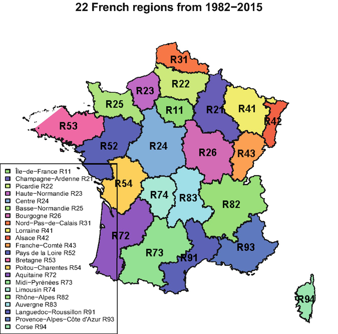

  

  The 22 regions in France between 1982 and 2015

We start by describing the Exposure. The Exposure measures the duration of an insurance policy in yearly units; sometimes it is also called years-at-risk. The shortest exposure in our data set is 0.0027 which corresponds to 1 day, and the longest exposure is 1 which corresponds to 1 year. Figure 13.2 (lhs, middle) shows a histogram and a boxplot of these exposures. In view of the histogram we conclude that roughly 1/4 of all policies have a full exposure of 1 calendar year, and all other policies are only partly exposed during the calendar year. From a practical insurance point of view this high ratio of partly exposed policies seems rather unusual. A further inspection of the data indicates that policy renewals during the year account for two separate records in the data set. Of course, such split policies should be merged to one yearly policy. Unfortunately, we do not have the necessary information to perform this merger, therefore, we need to work with the data as it is.

Fig. 13.2

(lhs) Histogram of Exposure, (middle) boxplot of Exposure, (rhs) number of observed claims ClaimNb of the French MTPL data

In Table 13.1 and Fig. 13.2 (rhs) we split the portfolio w.r.t. the number of claims. On 653’069 insurance policies (amounting to a total exposure of 341’090 years-at-risk) we do not have any claim, and on the remaining 24’938 policies (17’269 years-at-risk) we have at least one claim. The overall portfolio claim frequency (w.r.t. Exposure) is $\overline {\lambda }=7.35\%$.

Table 13.1 Split of the portfolio w.r.t. the number of claims

Table 13.2 VehBrand assignment

We study the split of this overall frequency $\overline {\lambda }=7.35\%$ across the different feature levels. This empirical analysis is crucial for the model choice in regression modeling.⁶ For the empirical analysis we provide 3 different types of graphs for each feature component (where applicable), these are given in Figs. 13.3, 13.4, 13.5, 13.6, 13.7, 13.8, 13.9, 13.10, and 13.11. The first graph (lhs) gives the split of the total exposure to the different feature levels, the second graph (middle) gives the average feature value in each French region (green meaning low and red meaning high),⁷ and the third graph (rhs) gives the observed average frequency per feature level. This observed frequency is obtained by dividing the total number of claims by the total exposure per feature level. The frequencies are complemented by confidence bounds of two standard deviations (shaded area). These confidence bounds correspond to twice the estimated standard deviations. The standard deviations are estimated under a Poisson assumption, thus, they are obtained by , where $\overline {\lambda }_k$ is the observed frequency and Exposure _k is the total exposure for a given feature level k. We note that in all frequency plots the y-axis ranges from 0% to 20%, except in the BonusMalus plot where the maximum is set to 60%, and the DrivAge plot where the maximum is set to 40%. From these plots we conclude that some levels have only a small underlying Exposure; BonusMalus leads to the highest variability in frequencies followed by DrivAge; and there is quite some heterogeneity.

Fig. 13.3

(lhs) Histogram of exposures per Area code, (middle) average Area code per Region, we map (A, …, F)↦(1, …, 6), (rhs) observed frequency per Area code

Fig. 13.4

(lhs) Histogram of exposures per VehPower, (middle) average VehPower per Region, (rhs) observed frequency per VehPower

Fig. 13.5

(lhs) Histogram of exposures per VehAge (censored at 20), (middle) average VehAge per Region, (rhs) observed frequency per VehAge

Fig. 13.6

(lhs) Histogram of exposures per DrivAge (censored at 90), (middle) average DrivAge per Region, (rhs) observed frequency per DrivAge (y-scale is different compared to the other frequency plots)

Fig. 13.7

(lhs) Histogram of exposures per BonusMalus level (censored at 150), (middle) average BonusMalus level per Region, (rhs) observed frequency per BonusMalus level (y-scale is different compared to the other frequency plots)

Fig. 13.8

(lhs) Histogram of exposures per VehBrand, (rhs) observed frequency per VehBrand; for VehBrand assignment we refer to Table 13.2

Fig. 13.9

(lhs) Histogram of exposures per VehGas, (middle) average VehGas per Region (diesel is green and regular red), (rhs) observed frequency per VehGas

Fig. 13.10

(lhs) Histogram of exposures per population Density (on log-scale), (middle) average population Density per Region, (rhs) observed frequency per population Density; in general, we always consider Density on the log-scale

Fig. 13.11

(lhs) Histogram of exposures Exposure, and (middle, rhs) observed claim frequencies per Region in France (prior to 2016)

Table 13.2 gives the assignment of the different VehBrand levels to car brands. This list has been compiled from the two data sets FreMTPLfreq and FreMTPL2freq contained in the R package CASdatasets [113], see Footnote 5.

Next, we analyze collinearity between the feature components. For this we calculate Pearson’s correlation and Spearman’s Rho for the continuous feature components, see Table 13.3. In general, these correlations are low, except for DrivAge vs. BonusMalus. Of course, the latter is very sensible because a BonusMalus level below 100 needs a certain number of driving years without claims. We give the corresponding boxplot in Fig. 13.12 (lhs) which confirms this negative correlation.

Fig. 13.12

Boxplots (lhs) BonusMalus vs. DrivAge, (rhs) log-Density vs. Area code; these plots are inspired by Fig. 2 in Lorentzen–Mayer [258]

Table 13.3 Correlations in feature components: top-right shows Pearson’s correlation; bottom-left shows Spearman’s Rho; Density is considered on the log-scale; significant correlations are boldface

Figure 13.12 (rhs) gives the boxplot of log-Density vs. Area code. From this plot we conclude that the area code has likely been set w.r.t. the log-Density. For our regression models this means that we can drop the area code information, and we should only work with Density. Nevertheless, we will use the area code to show what happens in case of collinear feature components, i.e., if we replace (A, …, F)↦(1, …, 6).

Figure 13.13 illustrates each continuous feature component w.r.t. the different VehBrands. Vehicle brands B10 and B11 (Mercedes, Chrysler and BMW) have more VehPower than other cars, B10 being more likely a diesel car, and vehicle brand B12 (Japanese and Korean cars) has comparably new cars in more densely populated French regions.

Fig. 13.13

Distribution of the variables VehPower, VehAge, DrivAge, BonusMalus, log-Density, VehGas for each car brand VehBrand, individually

More formally, the strength of dependence between categorical variables can be measured by Cramér’s V . Cramér’s V  is based on the χ ²-test of independence on contingency tables. We briefly explain this. Assume we have two-dimensional categorical features $\boldsymbol {x}=(x_1,x_2) \in \mathcal {X}$ having m ₁ and m ₂ levels, respectively. Let p _x describe the probability on $\mathcal {X}$ that a randomly chosen insurance policy takes feature x, and let $p_{x_1}$ and $p_{x_2}$ be the marginal distributions of p _x. If the two components of x are independent with these two marginals, then we have special (independence) distribution

$$\displaystyle \begin{aligned} \pi_{\boldsymbol{x}}=p_{x_1}p_{x_2} \qquad \text{ for all }\boldsymbol{x}=(x_1,x_2) \in \mathcal{X}. \end{aligned}$$

The χ ²-test for independence now analyzes p _x vs. π _x. Assume we have n observations. Denote by $n_{\boldsymbol {x}}=n_{x_1,x_2}$ the number of instances that have feature x = (x ₁, x ₂), and let $n_{x_1,\boldsymbol {\cdot }}$ and $n_{\boldsymbol {\cdot },x_2}$ be the corresponding marginal observations. The χ ²-test statistics is given by

$$\displaystyle \begin{aligned} \chi^2 = \sum_{\boldsymbol{x}=(x_1,x_2) \in \mathcal{X}} \frac{\left(n_{\boldsymbol{x}} - \frac{n_{x_1,\boldsymbol{\cdot}}~n_{\boldsymbol{\cdot}, x_2}}{n}\right)^2} {\frac{n_{x_1,\boldsymbol{\cdot}}~n_{\boldsymbol{\cdot}, x_2}}{n}}. \end{aligned}$$

Under the null hypothesis of having independence between the components of x, the test statistics χ ² converges in distribution to a χ ²-distribution with (m ₁ m ₂ − 1) degrees of freedom if we let the number of independently drawn instances go to infinity. Seven different proofs of this statement are given in Benhamou–Melot [30]. We scale the test statistics to the interval [0, 1] by dividing it by the comonotonic (maximal dependent) case and by the sample size n. This motivates Cramér’s V 

Section 7.2.3 of Cohen [78] gives a rule of thumb for small, medium and large dependence. Cohen [78] calls the association between x ₁ and x ₂ small if is less 0.1, it is of medium strength for of size 0.3, and it is a large effect if this value is around 0.5. Our results are presented in Table 13.4. Clearly, there is some association between VehBrand and both VehPower and VehAge, this can also be seen from Fig. 13.13, for the remaining variables the dependence is somewhat weaker. Not surprisingly, Cramér’s V  shows the largest value between Region and log-Density.

Table 13.4 Cramér’s V  for the categorical feature components vs. the categorized continuous components

In Fig. 13.14 we show the VehBrands in the different French Regions, Cramér’s V  is 0.13 for these two categorical variables, multiplying with gives a value bigger than 0.4 which is a considerable association according to Cohen [78]. We note that in some regions the French car brands B1 and B2 are very dominant, whereas on the Isle of Corse (R94) 80% of the cars in our portfolio are Japanese or Korean cars B12. Our portfolio has its biggest exposure in Region R24, see Fig. 13.11, in this region French cars are predominant.

Fig. 13.14

VehBrands in the different French Regions

Next, we study the claim sizes of this French MTPL example. Figure 13.15 shows the empirical density plot and the log-log plot. These two plots already illustrate the main difficulty we often face in claim size modeling. From the empirical density plot we observe that there are many payments of fixed size (red vertical lines) which do not match any absolutely continuous distribution function assumption. The log-log plot shows heavy-tailedness because we observe asymptotically a straight line with negative slope on the log-scale, this indicates regularly varying tails and, thus, the EDF is not a suitable model on the original observation scale.

Fig. 13.15

Empirical density and log-log plots of the observed claim amounts

Figure 13.16 gives the boxplots of the claim sizes per feature level (we omit the claims outside the whiskers because heavy-tailedness would distort the picture). The empirical mean in orange is much bigger than the median in red color, which also expresses the heavy-tailedness. From these plots we conclude that the claim sizes seem less sensitive in feature values which may question the use of a regression model for claim sizes.

Fig. 13.16

Boxplots of claim sizes per feature level: these plots omit the claims outside the whiskers; red color shows the median and orange color the empirical mean

Figure 13.17 shows the density plots for different feature levels. Interestingly, it seems that the features determine the sizes of the modes, for instance, if we focus on Area, Fig. 13.17 (top-left), we see that the area codes mainly influence the sizes of the modes. This may be interpreted by modes corresponding to different claim types which occur at different frequencies among the area codes.

Fig. 13.17

Empirical claim size densities split w.r.t. the different levels of the feature components

13.2 Swedish Motorcycle Data

Our second example considers the Swedish motorcycle data which originally has been used in Ohlsson–Johansson [290]. It is available through the R library CASdatasets [113], and it is called swmotorcycle. Listing 13.3 shows the data cleaning that we have used, and Listing 13.4 gives an excerpt of the cleaned data.

Listing 13.3 Data cleaning applied to the Swedish motorcycle data set

Listing 13.4 Excerpt of the Swedish motorcycle data set

We briefly describe the data. The data considers comprehensive insurance for motorcycles. This covers loss or damage of motorcycles other than collision, e.g., caused by theft, fire or vandalism. The data considers aggregated claims on feature levels for years 1994–1998. We have claims on 656 out of the 62’036 different features, thus, only slightly more than 1% of all feature combinations suffer a claim in the considered period.

We start by describing the available variables on lines 2–10 of Listing 13.4:

• 1. OwnerAge: age of motorcycle owner in {18, …, 70} years (we censor at 70 because of scarcity of data above);

• 2. Gender: gender of motorcycle owner either being Female or Male;

• 3. Area: 7 geographical Swedish zones being (1) central parts of Sweden’s three largest cities, (2) suburbs and middle-sized towns, (3) lesser towns except those in zones (5)–(7), (4) small towns and countryside except those in zones (5)–(7), (5) Northern towns, (6) Northern countryside, and (7) Gotland (Sweden’s largest island);

• 4. RiskClass: 7 ordered motorcycle classes received from the so-called EV ratio defined as (Engine power in kW × 100) / (Vehicle weight in kg +  75kg);

• 5. VehAge: age of motorcycle in {0, …, 30} years (we censor at 30);

• 6. BonusClass: ordered bonus-malus class from 1 to 7, entry level is 1;

• 7. Exposure: total exposure in yearly units, these exposures are aggregated for given feature combinations, resulting in total exposures [0.0274, 31.3397], the shortest entry referring to 10 days and the longest one to more than 31 years;

• 8. ClaimNb: number of claims N _i for a given feature;

• 9. ClaimAmount: total claim amount for a give feature (aggregated over all claims).

We start with a descriptive and exploratory analysis of the Swedish motorcycle data of Listing 13.4. We have n = 62′036 different feature combinations with positive Exposure. This Exposure is aggregated over individual policies with a fixed feature combination. We denote by N _i the number of claims on feature i, this corresponds to ClaimNb, and the total claim amount ClaimAmount is denoted by $S_i=\sum _{j=1}^{N_i} Z_{i,j}$, where Z _i,j are the individual claim sizes on feature i (in case of claims). The empirical claim frequency is $\bar {\lambda }=\sum _{i=1}^n N_i/\sum _{i=1}^n v_i=1.05\%$, and the average claim size is $\bar {\mu }=\sum _{i=1}^{n} S_i/\sum _{i=1}^{n}N_i = 24'641$ Swedish crowns SEK.

Figure 13.18 shows the boxplot over all Exposures and the claim counts on all insurance policies. We note that insurance claims are rare events for this product, because the empirical claim frequency is only $\bar {\lambda }= 1.05\%$.

Fig. 13.18

(lhs) Boxplot of Exposure on the log-scale (the horizontal line corresponds to 1 accounting year), (rhs) histogram of the number of observed claims ClaimNb per feature of the Swedish motorcycle data

Figures 13.19 and 13.20 give the marginal total exposures (split by gender), the marginal claim frequencies and the marginal average claim amounts for the covariate components OwnerAge, Area, RiskClass, VehAge and BonusClass. We observe that we have a very imbalanced portfolio between genders, only 11% of the total exposure is coming from females. The empirical claim frequency of females is 0.86% and the one of males is 1.08%. We note that the female claim frequency comes from (only) 61 claims (based on an exposure for female of 7’094 accounting years, versus 57’679 for male). Therefore, it is difficult to analyze females separately, and all marginal claim frequencies and claim sizes in Figs. 13.19 and 13.20 (middle and rhs) are analyzed jointly for both genders. If we run a simple Poisson GLM that only involves Gender as feature component, it turns out that the female frequency is 20% lower than the male frequency (remember we have the balance property on each dummy variable, see Example 5.12), but this variable should not be kept in the model on a 5% significance level. The same holds for claim amounts.

Fig. 13.19

(Top, middle and bottom rows) OwnerAge, Area, RiskClass: (lhs) histogram of exposures (split by gender), (middle) observed claim frequency, (rhs) boxplot of observed average claim amounts $\bar {\mu }_i=S_i/N_i$ of features with N _i > 0 (on log-scale)

Fig. 13.20

(Top and bottom rows) VehAge, BonusClass: (lhs) histogram of exposures (split by gender), (middle) observed claim frequency, (rhs) boxplot of observed average claim amounts $\bar {\mu }_i=S_i/N_i$ of features with N _i > 0 (on log-scale)

The empirical marginal frequencies in Figs. 13.19 and 13.20 (middle) are complemented with confidence bands of ± 2 standard deviations. From the plots we conclude that we should keep the explanatory variables OwnerAge, Area, RiskClass and VehAge, but the variable BonusClass does not seem to have any predictive power. At the first sight, this seems surprising because the bonus class encodes the past claims history. The reason that the bonus class is not needed for our claims is that we consider comprehensive insurance for motorcycles covering loss or damage of motorcycles other than collision (for instance, caused by theft, fire or vandalism), and the bonus class encodes collision claims.

For a regression analysis Zones 5 to 7 should be merged because of small exposures and a similar behavior, the same applies to RiskClass 6 and 7, and VehAge above 20.

Figure 13.21 shows the correlations between the features: (top) correlations between continuous features, (bottom), dependence between continuous features and the categorical Area features. We have some dependence, for instance, in Zone 1 (three largest Swedish cities) the motorcycles are more light (RiskClass) and less old. Older people drive less heavy motorcycles that are more old, and older motorcycles are less heavy.

Fig. 13.21

(Top) Correlations: top-right shows Pearson’s correlation; bottom-left shows Spearman’s Rho; (bottom) boxplots of OwnerAge, RiskClass, VehAge versus Area (where Zones 5–7 have been merged)

Figure 13.22 gives the empirical density, empirical distribution and log-log plot of average claim amounts $\bar {\mu }_i=S_i/N_i$. From the log-log plot we conclude that the average claim amounts are not heavy-tailed for this motorcycle insurance product.

Fig. 13.22

(lhs) Empirical density (middle) empirical distribution and (rhs) log-log plot of average claim amounts $\bar {\mu }_i=S_i/N_i$ of features with N _i > 0

13.3 Wisconsin Local Government Property Insurance Fund

The third example considers property insurance claims of the Wisconsin Local Government Property Insurance Fund (LGPIF). This data⁸ has been made available through the book project of Frees [135],⁹ and is also used in Lee et al. [236]. The Wisconsin LGPIF is an insurance pool that is managed by the Wisconsin Office of the Insurance Commissioner. This fund provides insurance protection to local governmental institutions such as counties, schools, libraries, airports, etc. It insures property claims for buildings and motor vehicles, and it excludes certain natural and man made perils like flood, earthquakes or nuclear accidents. We give a description of the data (we have applied some data cleaning to the original data).

Listing 13.5 Excerpt of the Wisconsin LGPIF data set

The special feature of this data is that we have a short claim description on line 11 of Listing 13.5. This description will allow us to better understand the claim type beyond just knowing the hazard type that has been affected.

Figure 13.23 gives the empirical density (upper-truncated at 50’000) and the log-log plot of the observed LGPIF claim amounts. Most claims are below 10’000, however, the log-log plot shows clearly that the data is heavy-tailed, the largest claim being 12’922’218 and 13 claims being above 1 million. These claims are further described by the features given in Listing 13.5.

Fig. 13.23

(lhs) Empirical density (upper-truncated at 50’000), (rhs) log-log plot of the observed LGPIF claim amounts

In our example we will not focus on modeling the claim sizes, but we rather aim at predicting the hazard types from the claim descriptions. There are 9 different hazard types: Fire, Lightning, Hail, Wind, WaterW, WaterNW, Vehicle, Vandalism and Misc. The last label contains all claims that cannot be allocated to one of the previous hazard types, and WaterW refers to weather related water claims and WaterNW to the non-weather related ones. If we only focus on this latter problem we have more data available as there is a training data set and a validation data set with hazard types and claim descriptions.¹⁰ In total we have 6’031 such claim descriptions, see Listing 13.6, which are studied in our text recognition Chap. 10.

Listing 13.6 Excerpt of the Wisconsin LGPIF claim descriptions

13.4 Swiss Accident Insurance Data

Our next example considers Swiss accident insurance data.¹¹ This data set is not publicly available. Swiss accident insurance is compulsory for employees, i.e., by law each employer has to sign an insurance contract to protect the employees against accidents. This insurance cover includes both work and leisure accidents, and it covers medical expenses and daily allowance. Listing 13.7 gives an excerpt of the data. Line BU indicates whether we have a workplace or a leisure accident, line 10 gives the medical expenses and line 12 shows the allowance expenses. In the subsequent analysis we only consider medical expenses.

Listing 13.7 Excerpt of the Swiss accident insurance data set

Sector indicates the labor sector of the insured company, AccQuart gives the accident quarter since leisure claims have a seasonal component, RepDel gives the reporting delay in yearly units, Age is the age of the injured (in 5 years buckets), and InjType and InjPart denote the injury type and the injured body part.

Figure 13.24 gives the empirical density (upper-truncated at 10’000) and the log-log plot of the observed Swiss accident insurance claim amounts. Most claims are below 5’000, however, the log-log plot shows some heavy-tailedness, the largest claim exceeding 1’300’000 CHF.

Fig. 13.24

(lhs) Empirical density (upper-truncated at 10’000), (rhs) log-log plot of the observed Swiss accident insurance claim amounts

Figure 13.25 shows the average claim amounts split w.r.t. the different feature components (top) Sector, AccQuart, RepDel, (bottom) Age, InjType, InjPart, and moreover, split by work and leisure accidents (in cyan and gray in the colored version). Typically, leisure accidents are more numerous and more expensive on average than accidents at the work place. From Fig. 13.25 (top, left) we observe considerable variability in average claim sizes between the different labor sectors (cyan bars), whereas average leisure claim sizes (gray bars) are similar across the different labor sectors. Average claim sizes considerably differ between injury types and injured body parts (bottom, middle and right), but they do not differ between work and leisure claims.

Fig. 13.25

Average claim amounts split w.r.t. the different feature components (top) Sector, AccQuart, RepDel, (bottom) Age, InjType, InjPart, and split by work and leisure accidents (cyan/gray in the colored version)

References

Benhamou, E., & Melot, V. (2018). Seven proofs of the Pearson Chi-squared independence test and its graphical interpretation. arXiv:1808.09171.
Cohen, J. (1988). Statistical power analysis for the behavioral sciences (2nd ed.) New York: Lawrence Erlbaum Associates.
Dutang, C., & Charpentier, A. (2018). CASdatasets R package vignette. Reference manual. Version 1.0-8, packaged 2018-05-20.
Frees, E. W. (2020). Loss data analytics. An open text authored by the Actuarial Community. https://ewfrees.github.io/Loss-Data-Analytics/
Lee, G. Y., Manski, S., & Maiti, T. (2020). Actuarial applications of word embedding models. ASTIN Bulletin, 50/1, 1–24.
Lorentzen, C., & Mayer, M. (2020). Peeking into the black box: An actuarial case study for interpretable machine learning. SSRN Manuscript ID 3595944. Version May 7, 2020.
Loser, F. (2020). Private communication.
Noll, A., Salzmann, R., & Wüthrich, M. V. (2018). Case study: French motor third-party liability claims. SSRN Manuscript ID 3164764. Version March 4, 2020.
Ohlsson, E., & Johansson, B. (2010). Non-life insurance pricing with generalized linear models. New York: Springer.
Author information
Authors and Affiliations
Rights and permissions
Open Access This chapter is licensed under the terms of the Creative Commons Attribution 4.0 International License (http://creativecommons.org/licenses/by/4.0/), which permits use, sharing, adaptation, distribution and reproduction in any medium or format, as long as you give appropriate credit to the original author(s) and the source, provide a link to the Creative Commons license and indicate if changes were made.
The images or other third party material in this chapter are included in the chapter's Creative Commons license, unless indicated otherwise in a credit line to the material. If material is not included in the chapter's Creative Commons license and your intended use is not permitted by statutory regulation or exceeds the permitted use, you will need to obtain permission directly from the copyright holder.
Copyright information
© 2023 The Author(s)
About this chapter
Cite this chapter
Wüthrich, M.V., Merz, M. (2023). Appendix B: Data and Examples. In: Statistical Foundations of Actuarial Learning and its Applications. Springer Actuarial. Springer, Cham. https://doi.org/10.1007/978-3-031-12409-9_13
Download citation
DOI: https://doi.org/10.1007/978-3-031-12409-9_13
Published:
Publisher Name: Springer, Cham
Print ISBN: 978-3-031-12408-2
Online ISBN: 978-3-031-12409-9
eBook Packages: Mathematics and StatisticsMathematics and Statistics (R0)