Inferences with Propositional Questions

Abstract

In the previous chapter we have seen how classical propositional logic can be extended with questions, leading to the inquisitive propositional logic InqB. In this section we will describe a natural deduction system for InqB and show this system to be sound and complete. We will also use this system to make some more general points about the role of questions in inference and about the intuitive significance of supposing or concluding a question. Lastly, we will show that proofs in our system have an interesting kind of constructive content: a proof can generally be seen as encoding a method for turning resolutions of the assumptions into a corresponding resolution of the conclusion.

In the previous chapter we have seen how classical propositional logic can be extended with questions, leading to the inquisitive propositional logic InqB. In this section we will describe a natural deduction system for InqB and show this system to be sound and complete. We will also use this system to make some more general points about the role of questions in inference and about the intuitive significance of supposing or concluding a question. Lastly, we will show that proofs in our system have an interesting kind of constructive content: a proof can generally be seen as encoding a method for turning resolutions of the assumptions into a corresponding resolution of the conclusion.

4.1 A Natural Deduction System for InqB

A natural deduction system for InqB is presented in Fig. 4.1. In these rules, the variables $\varphi ,\psi ,$ and $\chi$ range over all formulas, while $\alpha$ is restricted to classical formulas. We refer to the introduction rule for a connective $\circ$ as $(\circ \textsf {i})$, and to the elimination rule as $(\circ \textsf {e})$. As usual, those rules that discharge assumptions allow us to discharge an arbitrary number of occurrences of the assumption in the relevant sub-proof. We write $P:\Phi \vdash \psi$ to mean that P is a proof whose set of undischarged assumptions is included in $\Phi$ and whose conclusion is $\psi$, and we write $\Phi \vdash \psi$ to mean that a proof $P:\Phi \vdash \psi$ exists. Two formulas $\varphi$ and $\psi$ are provably equivalent, notation $\varphi \dashv \vdash \psi$, in case $\varphi \vdash \psi$ and $\psi \vdash \varphi$. Let us comment briefly on the rules of this system.

Fig. 4.1

A sound and complete natural-deduction system for InqB. In these rules, the variables $\varphi ,\psi ,$ and $\chi$ range over arbitrary formulas, while the variable $\alpha$ is restricted to range over classical formulas

Conjunction. Conjunction is handled by the usual introduction and elimination rules: from a conjunction we can infer either conjunct, and from both conjuncts we can infer the conjunction. The soundness of these rules corresponds to the following standard fact.

Proposition 4.1.1

$\Phi \models \varphi \wedge \psi \iff \Phi \models \varphi \text { and }\Phi \models \psi$.

Notice that these rules are not restricted to classical formulas: conjunctive questions such as ${?p}\wedge {?q}$ can be handled in inferences just like standard conjunctions.

Implication. Implication is also handled by the standard inference rules: from an implication together with its antecedent we can infer the consequent; conversely, if from the assumption of $\varphi$ we can infer $\psi$, we can discharge the assumption and conclude $\varphi \rightarrow \psi$. The soundness of these rules corresponds to the following fact, which captures the tight relation existing between implication and entailment.

Proposition 4.1.2

$\Phi \models \varphi \rightarrow \psi \iff \Phi ,\varphi \models \psi$.

Again, these rules are not restricted to classical formulas: implications involving questions can also be handled by means of the standard implication rules. This means that, e.g., in order to prove a dependence formula, say ${?p}\rightarrow {?q}$, we can proceed by assuming the determinant ?p and showing that from it we can derive the determined question, ?q. Conversely, if we have ${?p}\rightarrow {?q}$ as well as the determinant, ?p, we can on that basis infer the determined question, ?q.

Falsum. As usual, $\bot$ has no introduction rule, and can be eliminated to infer any formula. This corresponds to the fact that we have $\bot \models \varphi$ for all formulas $\varphi$, which in turn is a consequence of the fact that the inconsistent state $\emptyset$ always supports every formula.

Negation. As $\lnot \varphi$ is defined as $\varphi \rightarrow \bot$, the usual intuitionistic rules for negation, given in Fig. 4.2, follow as particular cases of the rules for implication.

Inquisitive disjunction. Inquisitive disjunction is handled by the standard natural deduction rules for disjunction: we can infer a disjunction from either disjunct and, conversely, whatever can be inferred from either disjunct can be inferred from the disjunction. The soundness of these rules corresponds to the following fact.

Proposition 4.1.3

and $\,\Phi ,\psi \models \chi$.

Classical disjunction. Figure 4.2 shows the derived rules for $\vee$. While both rules are standard, the elimination rule is restricted to conclusions that are classical formulas. Without this restriction, the rule would not be sound. E.g., we have $p\models {?p}$ and $\lnot p\models {?p}$, but $p\vee \lnot p\not \models {?p}$: indeed, the question ?p is logically resolved by both statements p and $\lnot p$, but not by the disjunction $p\vee \lnot p$.

Fig. 4.2

Derived rules for $\vee$ and $\lnot$, where $\alpha$ is restricted to classical formulas

Double negation elimination. We saw in the previous chapter (Proposition 3.4.10) that the double negation law is characteristic of statements. Thus, this rule reflects the fact that classical formulas are statements in InqB.

In fact, to obtain a complete proof system it is not strctly necessary to allow double negation elimination for all classical formulas: it would be sufficient to allow double negation for atoms, so as to let the system know that we are taking atomic sentences to be statements (cf. the discussion in Sect. 3.8). It would then be possible to infer $\alpha$ from $\lnot \lnot \alpha$ for any classical $\alpha$ on the basis of the rules for $\bot$, $\wedge$, and $\rightarrow$. While this is indeed the choice made in some work on inquisitive logic (e.g., Ciardelli and Roelofsen [1]), allowing double negation as a primitive rule for all classical formulas is quite natural, given our perspective of viewing InqB as a conservative extension of classical propositional logic; in this way, our system is an extension of a standard natural deduction system for classical logic (as given, e.g., in Gamut [2]). This ensures that any standard natural deduction proof in classical logic is also a proof in our system.

Split. The -split rule allows us to distribute a classical antecedent over an inquisitive-disjunctive consequent. This rule is backed by the -split equivalence

given by Proposition 3.7.14. As we discussed in detail on Sect. 3.7.3, this equivalence is a logical rendering of the fact that statements are specific, i.e., they correspond to specific pieces of information (Proposition 3.7.12). As we discussed in Sect. 2.6, this property can be seen as marking the crucial difference between statements and questions. Thus the -split rule has a clear conceptual significance which may perhaps not be obvious at first.

It is interesting to remark that the double negation rule and the -split rule capture different properties of statements in InqB: the former captures the fact that the logic of statements in InqB is classical, while the latter captures the idea that statements correspond to specific pieces of information. The latter idea seems constitutive of the inquisitive perspective, while the classicality of the underlying logic is not. Indeed, it is possible to build inquisitive logics based on non-classical logics of statements (see especially Punčochář [3,4,5], Ciardelli et al. [6]). In such logics, the double negation law may fail, but the -split equivalence remains valid.¹ $^,$²

Having discussed the significance of the inference rules, let us now illustrate how these rules can be used to build proofs of inquisitive entailments.

Example 4.1.4

As a first example, consider the following InqB-entailment:

$$p\leftrightarrow \lnot q\models {?p}\rightarrow {?q}.$$

This is valid: under the assumption that p and q have opposite truth values, it follows that whether q is the case is determined by whether p is the case. Here is a simple proof of this entailment in our natural deduction system (recall that  and  ):

In this proof, the steps which are not labeled involve only inferences with classical formulas. Since these coincide with inferences in classical propositional logic, we omit the standard details.

Example 4.1.5

As a second example, consider again the conditional dependence discussed in Sect. 2.3.3: in the die roll scenario, the range of the outcome determines what the outcome is, given that the outcome is prime. This fact can be captured as a logical entailment in InqB. Recall from the previous chapter (cf. Example 3.2.6 on Sect. 3.2 for the details) that we can formalize the scenario in a propositional language equipped with a set of atoms $\mathcal {P}=\{\textsf {one}, \dots , \textsf {six}\}$. We can then define the following statements as classical disjunctions of our atoms:

• $\textsf {low}:=\textsf {one}\vee \textsf {two}$;

• $\textsf {mid}:=\textsf {three}\vee \textsf {four}$;

• $\textsf {high}:=\textsf {five}\vee \textsf {six}$;

• $\textsf {prime}:=\textsf {two}\vee \textsf {three}\vee \textsf {five}$.

By using inquisitive disjunction we can also define the following questions:

• 

• .

The assumptions that the outcomes are jointly exhaustive and mutually exclusive possibilities are captured by the following formulas:

• $\textsf {exh}\;:=\;(\textsf {one}\vee \dots \vee \textsf {six})$;

• $\textsf {exc}\;:=\;\lnot (\textsf {one}\wedge \textsf {two})\wedge \lnot (\textsf {one}\wedge \textsf {three})\wedge \dots \wedge \lnot (\textsf {five}\wedge \textsf {six})$.

Let $\Gamma =\{\textsf {exh},\textsf {exc}\}$. Then the following entailment, which amounts to the conditional dependence of outcome on range given prime, is valid:

$$\Gamma ,\textsf {prime},\textsf {range}\,\models \,\textsf {outcome}.$$

Below is a proof of this entailment, where again we omit steps that involve only inferences in classical propositional logic.

4.2 Constructive Content of Proofs in InqB

Looking again at the two examples of proofs in the previous section, we can see that they are, in a certain sense, constructive. For instance, the second proof we saw does not just witness the fact that, under the given declarative assumptions, information of type range can be used to obtain information of type outcome: it actually describes how to use information of type range to obtain information of type outcome. In other words, the proof encodes a logical dependence function f (cf. Definition 3.6.15) that can be used to turn any given information of type range to corresponding information of type outcome. This is not just a feature of this particular proof, but a general fact: any inquisitive proof encodes a logical dependence function. To see how this works, let us write $\overline{\varphi }$ for a sequence $\varphi _1,\dots ,\varphi _n$ of formulas, and $\overline{\alpha }\in \mathcal {R}(\overline{\varphi })$ to mean that $\overline{\alpha }$ is a sequence $\alpha _1,\dots ,\alpha _n$ such that $\alpha _i\in \mathcal {R}(\varphi _i)$. We have the following result [8].

Theorem 4.2.1

(Existence of a resolution algorithm) If $P:\overline{\varphi }\vdash \psi$, we can define inductively on P a procedure $F_P$ which maps each $\overline{\alpha }\in \mathcal {R}(\overline{\varphi })$ to a proof $\,F_P(\overline{\alpha }):\overline{\alpha }\vdash \beta$ having as conclusion a resolution $\beta \in \mathcal {R}(\psi )$.

Proof

Let us describe how to construct the procedure $F_P$ inductively on P. We distinguish a number of cases depending on the last rule applied in P.

• $\psi$ is an undischarged assumption $\varphi _i$. In this case, any resolution $\overline{\alpha }\in \mathcal {R}(\overline{\varphi })$ contains a resolution $\alpha _i$ of $\varphi _i$ by definition. So, we can just let $F_P$ map $\overline{\alpha }$ to the trivial proof $Q:\overline{\alpha }\vdash \alpha _i$ which consists only of the assumption $\alpha _i$.

• $\psi =\chi \wedge \xi$ was obtained by $(\wedge \textsf {i})$ from $\chi$ and $\xi$. Then the immediate subproofs of P are a proof $P':\overline{\varphi }\vdash \chi$ and a proof $P'':\overline{\varphi }\vdash \xi$, for which the induction hypothesis gives two procedures $F_{P'},F_{P''}$. Now take any resolution $\overline{\alpha }$ of $\overline{\varphi }$. We have $F_{P'}(\overline{\alpha }):\overline{\alpha }\vdash \beta$ and $F_{P'}(\overline{\alpha }):\overline{\alpha }\vdash \gamma$, where $\beta \in \mathcal {R}(\chi )$ and $\gamma \in \mathcal {R}(\xi )$. By extending these proofs with an application of $(\wedge \textsf {i})$, we get a proof $Q:\overline{\alpha }\vdash \beta \wedge \gamma$. Since $(\beta \wedge \gamma )\in \mathcal {R}(\chi \wedge \xi )$, we can let $F_P(\overline{\alpha }):=Q$.

• $\psi =\chi \rightarrow \xi$ was obtained by $(\rightarrow \!\!\textsf {i})$. Then the immediate subproof of P is a proof $P':\overline{\varphi },\chi \vdash \xi$, for which the induction hypothesis gives a procedure $F_{P'}$. Now take any resolution $\overline{\alpha }$ of $\overline{\varphi }$. Suppose $\beta _1,\dots ,\beta _m$ are the resolutions of $\chi$. For $1\le i\le m$, the sequence $\overline{\alpha },\beta _i$ is a resolution of $\overline{\varphi },\chi$, and so we have $F_{P'}(\overline{\alpha },\beta _i):\overline{\alpha },\beta _i\vdash \gamma _i$ for some resolution $\gamma _i$ of $\xi$. Extending this proof with an application of $(\rightarrow \!\!\textsf {i})$, we have a proof $Q_i:\overline{\alpha }\vdash \beta _i\rightarrow \gamma _i$. Since this is the case for $1\le i\le n$, by several applications of the rule $(\wedge \textsf {i})$ we obtain a proof $Q:\overline{\alpha }\vdash (\beta _1\rightarrow \gamma _1)\wedge \dots \wedge (\beta _m\rightarrow \gamma _m)$. By construction, $(\beta _1\rightarrow \gamma _1)\wedge \dots \wedge (\beta _m\rightarrow \gamma _m)$ is a resolution of $\chi \rightarrow \xi$, and so we can let $F_P(\overline{\alpha }):=Q$.

• was obtained by   from one of the disjuncts. Without loss of generality, let us assume it is $\chi$. Thus, the immediate subproof of P is a proof $P':\overline{\varphi }\vdash \chi$, for which the induction hypothesis gives a procedure $F_{P'}$. Now take any resolution $\overline{\alpha }$ of $\overline{\varphi }$. The induction hypothesis gives us a proof $F_{P'}(\overline{\alpha }):\overline{\alpha }\vdash \beta$ for some $\beta \in \mathcal {R}(\chi )$. Since $\beta$ is also a resolution of , we can simply let $F_{P}(\overline{\alpha }):=F_{P'}(\overline{\alpha })$.

• $\psi$ was obtained by $(\wedge \textsf {e})$ from $\psi \wedge \chi$. Then the immediate subproof of P is a proof $P':\overline{\varphi }\vdash \psi \wedge \chi$, and the induction hypothesis gives a procedure $F_{P'}$. For any resolution $\overline{\alpha }$ of $\overline{\varphi }$, we have $F_{P'}(\overline{\alpha }):\overline{\alpha }\vdash \beta$, where $\beta \in \mathcal {R}(\psi \wedge \chi )$. By definition of resolutions for a conjunction, $\beta$ is of the form $\gamma \wedge \gamma '$ where $\gamma \in \mathcal {R}(\psi )$ and $\gamma '\in \mathcal {R}(\chi )$. Extending $F_{P'}(\overline{\alpha })$ with an application of $(\wedge \textsf {e})$ we have a proof $Q:\overline{\alpha }\vdash \gamma$. Since $\gamma \in \mathcal {R}(\psi )$, we can just let $F_P(\overline{\alpha }):=Q$.

• $\psi$ was obtained by $(\rightarrow \!\!\textsf {e})$  from $\chi$ and $\chi \rightarrow \psi$. Then the immediate subproofs of P are a proof $P':\overline{\varphi }\vdash \chi$, and a proof $P'':\overline{\varphi }\vdash \chi \rightarrow \psi$, for which the induction hypothesis gives procedures $F_{P'}$ and $F_{P''}$. Now consider a resolution $\overline{\alpha }$ of $\overline{\varphi }$. We have $F_{P'}(\overline{\alpha }):\overline{\alpha }\vdash \beta$ where $\beta \in \mathcal {R}(\chi )$, and a proof $F_{P''}(\overline{\alpha }):\overline{\alpha }\vdash \gamma$, where $\gamma \in \mathcal {R}(\chi \rightarrow \psi )$. Now, if $\mathcal {R}(\chi )=\{\beta _1,\dots ,\beta _m\}$, then $\beta =\beta _i$ for some i, and by definition of the resolutions of an implication, $\gamma =(\beta _1\rightarrow \gamma _1)\wedge \dots \wedge (\beta _n\rightarrow \gamma _m)$ where $\{\gamma _1,\dots ,\gamma _n\}\subseteq \mathcal {R}(\psi )$. Now, extending $F_{P''}(\overline{\alpha })$ with an application of $(\wedge \textsf {e})$ we obtain a proof $Q'':\overline{\alpha }\vdash \beta _i\rightarrow \gamma _i$. Finally, combining this proof with $F_{P'}(\overline{\alpha })$ and applying $(\rightarrow \!\!\textsf {e})$, we obtain a proof $Q:\overline{\alpha }\vdash \gamma _i$. Since the conclusion of this proof is a resolution of $\psi$, we can let $F_P(\overline{\alpha }):=Q$.

• $\psi$ was obtained by  from. Then the immediate subproofs of P are: a proof ; a proof $P'':\overline{\varphi },\chi \vdash \psi$; and a proof $P''':\overline{\varphi },\xi \vdash \psi$, for which the induction hypothesis gives procedures $F_{P'}$, $F_{P''}$, and $F_{P'''}$. Now take a resolution $\overline{\alpha }$ of $\overline{\varphi }$. We have $F_{P'}(\overline{\alpha }):\overline{\alpha }\vdash \beta$ for some . Without loss of generality, assume that $\beta \in \mathcal {R}(\chi )$. Then the sequence $\overline{\alpha },\beta$ is a resolution of $\overline{\varphi },\chi$. Thus, we have $F_{P''}(\overline{\alpha },\beta ):\overline{\alpha },\beta \vdash \gamma$ for some $\gamma \in \mathcal {R}(\psi )$. Now, by substituting any undischarged assumption of $\beta$ in the proof $F_{P''}(\overline{\alpha },\beta )$ by an occurrence of the proof $F_{P'}(\overline{\alpha })$, we obtain a proof $Q:\overline{\alpha }\vdash \gamma$ having a resolution of $\psi$ as its conclusion, and we can let $F_P(\overline{\alpha }):=Q$.

• $\psi$ was obtained by $(\bot \textsf {e})$. This means that the immediate subproof of P is a proof $P':\overline{\varphi }\vdash \bot$, for which the induction hypothesis gives a method $F_{P'}$. Now take any resolution $\overline{\alpha }$ of $\overline{\varphi }$. Since $\mathcal {R}(\bot )=\{\bot \}$, we have $F_{P'}(\overline{\alpha }):\overline{\alpha }\vdash \bot$. Now take any $\beta \in \mathcal {R}(\psi )$ (notice that, by definition, the set of resolutions of a formula is always non-empty): by extending the proof $F_{P'}(\overline{\alpha })$ with an application of $(\bot \textsf {e})$, we obtain a proof $Q:\overline{\alpha }\vdash \beta$. Since $\beta \in \mathcal {R}(\psi )$, we can let $F_P(\overline{\alpha }):=P$.

•  was obtained by an application of the -split rule from , where $\alpha \in \mathcal {L}^{\textsf {P}}_c$. Then, the immediate subproof of P is a proof 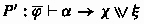, for which the induction hypothesis gives a method $F_{P'}$. Using the fact that $\mathcal {R}(\alpha )=\{\alpha \}$ (since $\alpha$ is a classical formula) it is easy to verify that . Therefore, we can simply let $F_P:=F_{P'}$.

• $\alpha \in \mathcal {L}^{\textsf {P}}_c$ was obtained by double negation elimination from $\lnot \lnot \alpha$. In this case, the immediate subproof of P is a proof $P':\overline{\varphi }\vdash \lnot \lnot \alpha$, for which the induction hypothesis gives a method $F_{P'}$. Since $\lnot \lnot \alpha$ is a classical formula, we have $\mathcal {R}(\lnot \lnot \alpha )=\{\lnot \lnot \alpha \}$. Thus, for any resolution $\overline{\beta }$ of $\overline{\varphi }$ we have $F_{P'}(\overline{\beta }):\overline{\beta }\vdash \lnot \lnot \alpha$. Extending this proof with an application of double negation elimination we obtain a proof $Q:\overline{\beta }\vdash \alpha$. Since $\alpha$ is a classical formula and thus $\mathcal {R}(\alpha )=\{\alpha \}$, we can then let $F_P(\overline{\beta }):=Q$.   $\square$

This result shows that a proof P in our system may be seen as a template $F_P$ for producing classical proofs, where questions serve as placeholders for generic information of the corresponding type. As soon as the assumptions of the proof are instantiated to particular resolutions, this template can be instantiated to a classical proof which infers some specific resolution of the conclusion. The idea is rendered by the following scheme:

We refer to the proof $F_P(\overline{\alpha })$ as the resolution of the proof P on the input $\overline{\alpha }$. Now, let us denote by $f_P$ the function that maps a resolution $\overline{\alpha }\in \mathcal {R}(\overline{\varphi })$ to the conclusion of the proof $F_P(\overline{\alpha })$. By definition, we have $f:\mathcal {R}(\overline{\varphi })\rightarrow \mathcal {R}(\psi )$. Moreover, for any $\overline{\alpha }\in \mathcal {R}(\overline{\varphi })$, we have $F_P(\overline{\alpha }):\overline{\alpha }\vdash f_P(\overline{\alpha })$, and thus, by the soundness of our proof system, we have $\overline{\alpha }\models f_P(\overline{\alpha })$. This shows that the function $f_P$ determined by the proof P is a logical dependence function from $\overline{\varphi }$ to $\psi$, in the sense of Definition exrefdef:depfunctionsets.

Corollary 4.2.2

(Inquisitive proofs encode dependence functions) If $P:\Phi \vdash \psi$, then inductively on P we can define a logical dependence function

.

This connection is reminiscent of the proofs-as-programs correspondence known for intuitionistic logic. As discovered by Curry [9] and Howard [10], in intuitionistic logic formulas may be regarded as types of a certain type theory, extending the simply typed lambda calculus. A proof $P:\varphi \vdash \psi$ in intuitionistic logic may be identified with a term $t_P$ of this type theory which describes a function that maps objects of type $\varphi$ to objects of type $\psi$. The situation is similar for InqB, except that now, formulas play double duty. On the one hand, formulas may be still be regarded as types. On the other hand, the elements of a type $\varphi$ may in turn be identified with certain formulas, namely, the resolutions of $\varphi$. As in intuitionistic logic, a proof $P:\varphi \vdash \psi$ determines a function $f_P$ from objects of type $\varphi$ to objects of type $\psi$; but since these objects may now be identified with classical formulas, the function $f_P$ is now defined within the language of classical propositional logic, i.e., we have $f_P:\mathcal {L}^{\textsf {P}}_c\rightarrow \mathcal {L}^{\textsf {P}}_c$.

4.3 Completeness

By showing that each inference rule of our proof system is sound, the discussion in Sect. 4.1 implies the soundness of our proof system as a whole.

Proposition 4.3.1

(Soundness) If $\Phi \vdash \psi$, then $\Phi \models \psi$.

In this section, we will be concerned with establishing the converse implication, i.e., with proving the following theorem.

Theorem 4.3.2

(Completeness) If $\Phi \models \psi$, then $\Phi \vdash \psi$.

There are multiple strategies to obtain this result. One proof (see Ciardelli and Roelofsen [11], Ciardelli [12]) follows the format of completeness proofs for intuitionistic and intermediate logics. Another strategy (see Ciardelli [13]) relies crucially on the normal form result and the fact that our proof system includes a complete system for classical propositional logic. In this section we present yet another proof. The advantages of this proof are that it is completely self-contained and that it can be extended straightforwardly to the setting of inquisitive modal logic (see Ciardelli [14, 15]).

The strategy of the proof can be summarized as follows. First, we will define a canonical model having complete theories of classical formulas as its possible worlds. Second, we will prove an analogue of the truth-lemma, the support lemma, which connects support in the canonical model with provability in our system. Finally, we will show that when a formula $\psi$ cannot be derived from a set $\Phi$, we can define a corresponding information state in the canonical model that supports $\Phi$ but not $\psi$.

4.3.1 Preliminary Results

Let us start out by establishing a few important facts about our proof system. First, notice that, if we leave out the rules of $\lnot \lnot$-elimination and -split, what we have is a complete system for intuitionistic propositional logic, with   in the role of intuitionistic disjunction. Thus, we have the following fact.

Lemma 4.3.3

(Intuitionistic entailments are provable) If $\Phi$ entails $\psi$ in intuitionistic propositional logic when   is identified with intuitionistic disjunction, then $\Phi \vdash \psi$.

Second, our proof system allows us to prove the equivalence between a formula and its normal form.

Lemma 4.3.4

(Provability of normal form) For any $\varphi$,.

Proof

The proof is by induction on $\varphi$. The basic cases for atoms and $\bot$ are trivial, and so is the inductive case for . So, only the inductive cases for conjunction and implication remain to be proved. Consider two formulas $\varphi$ and $\psi$, with $\mathcal {R}(\varphi )=\{\alpha _1,\dots ,\alpha _n\}$ and $\mathcal {R}(\psi )=\{\beta _1,\dots ,\beta _m\}$. Let us make the induction hypothesis that and , and let us consider the conjunction $\varphi \wedge \psi$ and the implication $\varphi \rightarrow \psi$.

• Conjunction. From the induction hypothesis and the rules for $\wedge$ we get

  

  Since the distributivity of conjunction over disjunction is provable in intuitionistic logic, by Lemma 4.3.3 we have

  

  And we are done, since by definition $\mathcal {R}(\varphi \wedge \psi )=\{\alpha _i\wedge \beta _j\,|\, i\le n, j\le m\}$.

• Implication. From the induction hypothesis and the rules for $\rightarrow$ we get

  

  By intuitionistic reasoning, we obtain the following:

  

  Now, since any resolution is a classical formula, it is easy to show using the -split rule that

  

  Since this is the case for for $1\le i\le n$, the rules for $\wedge$ yield

  

  Finally, using again the provable distributivity of $\wedge$ over , we get

  

  By definition of resolutions for an implication, the formula on the right is precisely . This completes the inductive proof.   $\square$

As a corollary, a formula may always be derived from each of its resolutions.

Corollary 4.3.5

For every $\varphi \in \mathcal {L}^{\textsf {P}}$, if $\alpha \in \mathcal {R}(\varphi )$ then $\alpha \vdash \varphi$.

Proof

Let $\mathcal {R}(\varphi )=\{\alpha _1,\dots ,\alpha _n\}$. By means of the rule , from $\alpha _i$ we can infer , and thus, by the previous lemma, we can infer $\varphi$.   $\square$

Another consequence of Lemma 4.3.4 is that, if $\psi$ in combination with other assumptions fails to yield a conclusion, this failure can always be traced to a specific resolution of $\psi$.

Lemma 4.3.6

If $\,\Phi ,\psi \not \vdash \chi \,$, then $\,\Phi ,\alpha \not \vdash \chi \,$ for some $\,\alpha \in \mathcal {R}(\psi )$.

Proof

We show the contrapositive: if $\Phi ,\alpha \vdash \chi$ for all $\alpha \in \mathcal {R}(\psi )$, then $\Phi ,\psi \vdash \chi$. Let $\mathcal {R}(\psi )=\{\alpha _1,\dots ,\alpha _n\}$. The rule  ensures that if we have $\Phi ,\alpha _i\vdash \chi$ for $1\le i\le n$ we also have . Since the previous lemma gives , we also get $\Phi ,\psi \vdash \chi$.   $\square$

The next lemma extends this result from a single assumption to the whole set.

Lemma 4.3.7

(Traceable deduction failure) If $\Phi \not \vdash \psi$, there is some resolution $\Gamma \in \mathcal {R}(\Phi )$ such that $\Gamma \not \vdash \psi$.

Proof

Let us fix an enumeration of $\Phi$, say $(\varphi _n)_{n\in \mathbb {N}}$.³ We are going to define a sequence $(\alpha _n)_{n\in \mathbb {N}}$ of classical formulas in $\mathcal {L}^{\textsf {P}}$ such that, for all $n\in \mathbb {N}$:

• $\alpha _n\in \mathcal {R}(\varphi _n)$;

• $\{\alpha _i\,|\,i\le n\}\cup \{\varphi _i\,|\,i> n\}\not \vdash \psi$.

Let us apply inductively the previous lemma. Assume we have defined $\alpha _i$ for $i<n$ and let us proceed to define $\alpha _n$. The induction hypothesis tells us that $\{\alpha _i\,|\,i<n\}\cup \{\varphi _i\,|\,i\ge n\}\not \vdash \psi$, that is, $\{\alpha _i\,|\,i<n\}\cup \{\varphi _i\,|\,i> n\},\varphi _n\not \vdash \psi$. Now the previous lemma tells us that we can “specify” the formula $\varphi _n$ to a resolution, i.e., we can find a formula $\alpha _n\in \mathcal {R}(\varphi _n)$ and $\{\alpha _i\,|\,i<{n}\}\cup \{\varphi _i\,|\,i> n\},\alpha _n\not \vdash \psi$. This means that $\{\alpha _i\,|\,i\le {n}\}\!\cup \!\{\varphi _i\,|\,i> n\}\not \vdash \psi$, completing the inductive proof.

Now let $\Gamma :=\{\alpha _n\,|\,n\in \mathbb {N}\}$. By construction, $\Gamma \in \mathcal {R}(\Phi )$. Moreover, we claim that $\Gamma \not \vdash \psi$. To see this, suppose towards a contradiction $\Gamma \vdash \psi$: then for some n it should be the case that $\alpha _1,\dots ,\alpha _n\vdash \psi$; but this is impossible, since by construction we have $\{\alpha _1,\dots ,\alpha _n\}\cup \{\varphi _{i}\,|\,i>n\}\not \vdash \psi$. Thus, $\Gamma \not \vdash \psi$.   $\square$

Using the existence of the Resolution Algorithm (Theorem 4.2.1) on the one hand, and the Traceable Failure Lemma on the other, we obtain an analogue of the Resolution Theorem (Theorem 3.7.17) for provability: a set of assumptions $\Phi$ derives a formula $\psi$ iff any resolution of $\Phi$ derives some resolution of $\psi$.

Lemma 4.3.8

(Resolution Lemma)$\Phi \vdash \psi \iff$ for all $\Gamma \in \mathcal {R}(\Phi )$ there is $\alpha \in \mathcal {R}(\psi )$ such that $\Gamma \vdash \alpha$.

Proof

The left-to-right direction of the lemma follows immediately from Theorem 4.2.1. Indeed, suppose there is a $P:\Phi \vdash \psi$ and let $\Gamma \in \mathcal {R}(\Phi )$: the theorem describes how to use P and $\Gamma$ to construct a proof of $\Gamma \vdash \alpha$ for some $\alpha \in \mathcal {R}(\psi )$.

For the converse, suppose $\Phi \not \vdash \psi$: the previous lemma tells us that there is a resolution $\Gamma \in \mathcal {R}(\Phi )$ such that $\Gamma \not \vdash \psi$. Since from any resolution $\alpha \in \mathcal {R}(\psi )$ we can derive $\psi$ (Corollary 4.3.5), we must also have $\Gamma \not \vdash \alpha$ for every $\alpha \in \mathcal {R}(\psi )$. Thus, it is not the case that any resolution of $\Phi$ derives some resolution of $\psi$.   $\square$

The next lemma shows that the Split Property is shared by provability, at least for the case in which the assumptions are classical formulas.

Lemma 4.3.9

(Provable Split) If $\Gamma$ is a set of classical formulas and , then $\Gamma \vdash \varphi$ or $\Gamma \vdash \psi$.

Proof

Suppose . Since $\Gamma$ is a set of classical formulas, Proposition 3.6.20 ensures that $\mathcal {R}(\Gamma )=\Gamma$. So, by Lemma 4.3.8 we have $\Gamma \vdash \beta$ for some . Since we have either $\beta \in \mathcal {R}(\varphi )$ or $\beta \in \mathcal {R}(\psi )$. In the former case, by Corollary 4.3.5 we have $\beta \vdash \varphi$, and thus also $\Gamma \vdash \varphi$. In the latter case, we have $\beta \vdash \psi$ and thus $\Gamma \vdash \psi$.   $\square$

4.3.2 Canonical Model

Let us now turn to the definition of our canonical model for InqB. As usual in classical and modal logic, we will construct our possible worlds out of complete theories. However, in our setting it is convenient to work with complete theories taken not from the full language, but from its classical fragment, $\mathcal {L}^{\textsf {P}}_c$.

Definition 4.3.10

(Theories of classical formulas) A theory of classical formulas is a set $\Gamma \subseteq \mathcal {L}^{\textsf {P}}_c$ which is closed under deduction of classical formulas, that is, if $\alpha \in \mathcal {L}^{\textsf {P}}_c$ and $\Gamma \vdash \alpha$ then $\alpha \in \Gamma$.

Definition 4.3.11

(Complete theories of classical formulas) A complete theory of classical formulas is a theory of classical formulas $\Gamma$ s.t.:

• $\bot \not \in \Gamma$;

• for any $\alpha \in \mathcal {L}^{\textsf {P}}_c$, either $\alpha \in \Gamma$ or $\lnot \alpha \in \Gamma$.

The following lemma is essentially just Lindenbaum’s lemma for classical propositional logic, which can be proved by means of the usual completion procedure.

Lemma 4.3.12

If $\Gamma \subseteq \mathcal {L}^{\textsf {P}}_c$ and $\Gamma \not \vdash \bot$ then $\Gamma \subseteq \Delta$ for some complete theory of classical formulas $\Delta$.

If S is a set of theories of classical formulas, we will denote by $\bigcap S$ the intersection of all the theories $\Gamma \in S$, with the convention that the intersection of the empty set of theories is the set of all classical formulas: $\bigcap \emptyset =\mathcal {L}^{\textsf {P}}_c$. A simple fact that will be useful in our proof is that $\bigcap S$ is itself a theory of classical formulas.

Lemma 4.3.13

If S is a set of theories of classical formulas, $\bigcap S$ is a theory of classical formulas.

Proof

It is obvious that $\bigcap S$ is a set of classical formulas. Moreover, suppose $\bigcap S\vdash \alpha$ and $\alpha$ is a classical formula. Take any $\Theta \in S$: since $\bigcap S\subseteq \Theta$, we also have $\Theta \vdash \alpha$, and since $\Theta$ is a theory of classical formulas, we have $\alpha \in \Theta$. Since this is the case for all $\Theta \in S$, we have $\alpha \in \bigcap S$.   $\square$

Our canonical model will have complete theories of classical formulas as worlds, and the canonical valuation will equate truth at a world with membership in it.

Definition 4.3.14

(Canonical model) The canonical model for InqB is the model $M^c=\langle W^c,V^c\rangle$ defined as follows:

• $W^c$ is the set of complete theories of classical formulas;

• $V^c:W^c\times \mathcal {P}\rightarrow \{0,1\}$ is defined by $V^c(\Delta ,p)=1\iff p\in \Delta$.

4.3.3 Completeness

Usually, the next step in the completeness proof is to prove the truth lemma, a result connecting truth at a possible world in the canonical model with provability from that world. However, in inquisitive semantics the fundamental semantic notion is not truth at a possible world, but support at an information state. Thus, what we need is a support lemma that characterizes the notion of support at a state in $M^c$ in terms of provability. What should this characterization be?

We may think of the information available in a state S as being captured by those statements that are true at all the worlds in S. Syntactically, truth at a world will correspond to membership in it. Thus, the information available in a state S is captured syntactically by the theory of classical formulas $\bigcap S$, which consists of those statements that belong to all the worlds in S.

For a formula $\varphi$, to be supported at S is to be settled by the information available in S. Syntactically, this would correspond to $\varphi$ being derivable from $\bigcap S$. Thus, we expect the following connection: $S\models \varphi \iff \bigcap S\vdash \varphi$. The following lemma states that this connection indeed holds.

Lemma 4.3.15

(Support Lemma) For any state $S\subseteq W^c$ and any $\varphi \in \mathcal {L}^{\textsf {P}}$:

$$S\models \varphi \iff \bigcap S\vdash \varphi .$$

Proof

The proof is by induction on $\varphi$, simultaneously for all $S\subseteq W^c$.

• Atoms. By the support clause for atoms, we have $S\models p\iff V^c(\Gamma ,p)=1$ for all $\Gamma \in S$. By definition of the canonical valuation, this is the case if and only if $p\in \Gamma$ for all $\Gamma \in S$, i.e., if and only if $p\in \bigcap S$. Finally, by Lemma 4.3.13 we have $p\in \bigcap S\iff \bigcap S\vdash p$.

• Falsum. Suppose $S\models \bot$. This means that $S=\emptyset$. Recalling that we have defined $\bigcap \emptyset$ to be the set $\mathcal {L}^{\textsf {P}}_c$ of all classical formulas, we have $\bigcap S\vdash \bot$. Conversely, suppose $S\not \models \bot$, that is, $S\ne \emptyset$. Then, take a $\Gamma \in S$: $\bigcap S\subseteq \Gamma$, and since $\Gamma \not \vdash \bot$ by definition, also $\bigcap S\not \vdash \bot$.

• Conjunction. The inference rules for conjunction imply that a conjunction is provable from a set of assumptions iff both of its conjuncts are. Using this fact and the induction hypothesis, we obtain: $S\models {\varphi \wedge \psi }\iff S\models \varphi \text { and }S\models \psi \iff \bigcap S\vdash \varphi \text { and }\bigcap S\vdash \psi \iff \bigcap S\vdash \varphi \wedge \psi$.

• Implication. Suppose $\bigcap S\vdash (\varphi \rightarrow \psi )$. Consider any state $T\subseteq S$ with $T\models \varphi$. By induction hypothesis, this means that $\bigcap T\vdash \varphi$. Since $T\subseteq S$, we have $\bigcap S\subseteq \bigcap T$, and since we are assuming $\bigcap S\vdash (\varphi \rightarrow \psi )$, also $\bigcap T\vdash (\varphi \rightarrow \psi )$. Now, since from $\bigcap T$ we can derive both $\varphi$ and $\varphi \rightarrow \psi$, by an application of $(\rightarrow \!\!\textsf {e})$ we can also derive $\psi$. Hence, by induction hypothesis we have $T\models \psi$. Since T was an arbitrary substate of S, we have shown that $S\models (\varphi \rightarrow \psi )$.

  For the converse, suppose $\bigcap S\not \vdash (\varphi \rightarrow \psi )$. By the rule $(\rightarrow \!\textsf {i})$, this implies that $\bigcap S,\varphi \not \vdash \psi$. Lemma 4.3.6 then ensures that there is an $\alpha \in \mathcal {R}(\varphi )$ such that $\bigcap S,\alpha \not \vdash \psi$.

  Now let $T_\alpha =\{\Gamma \in S\,|\,\alpha \in \Gamma \}$. First, we have $\alpha \in \bigcap T_\alpha$, whence $\bigcap T_\alpha \vdash \varphi$ by Corollary 4.3.5. By induction hypothesis we then have $T_\alpha \models \varphi$. Now, if we can show that $\bigcap T_\alpha \not \vdash \psi$ we are done. For then, the induction hypothesis gives $T_\alpha \not \models \psi$: this would mean that $T_\alpha$ is a substate of S that supports $\varphi$ but not $\psi$, showing that $S\not \models (\varphi \rightarrow \psi )$.

  So, we are left to show that $\bigcap T_\alpha \not \vdash \psi$. Towards a contradiction, suppose $\bigcap T_\alpha \vdash \psi$. Since $\bigcap T_\alpha$ is a set of classical formulas, it is a resolution of itself. Thus, Lemma 4.3.8 tells us that $\bigcap T_\alpha \vdash \beta$ for some resolution $\beta \in \mathcal {R}(\psi )$, which by Lemma 4.3.13 amounts to $\beta \in \bigcap T_\alpha$. So, for any $\Gamma \in T_\alpha$ we have $\beta \in \Gamma$, and thus also $(\alpha \rightarrow \beta )\in \Gamma$, since $\Gamma$ is closed under deduction of classical formulas and $\beta \vdash (\alpha \rightarrow \beta )$ by $({\rightarrow }\textsf {i})$. Now consider any $\Gamma \in S-T_\alpha$: this means that $\alpha \not \in \Gamma$ and so $\lnot \alpha \in \Gamma$ since $\Gamma$ is complete; but then we have $(\alpha \rightarrow \beta )\in \Gamma$, because $\Gamma$ is closed under deduction of classical formulas and $\lnot \alpha \vdash (\alpha \rightarrow \beta )$ by the rules $(\lnot \textsf {e})$, $(\bot \textsf {e})$, and $({\rightarrow }\textsf {i})$. We have thus shown that $(\alpha \rightarrow \beta )\in \Gamma$ for any $\Gamma \in S$, whether $\Gamma \in T_\alpha$ or $\Gamma \in S-T_\alpha$. We can then conclude $(\alpha \rightarrow \beta )\in \bigcap S$, whence by $({\rightarrow }\textsf {e})$ we have $\bigcap S,\alpha \vdash \beta$. Since $\beta \in \mathcal {R}(\psi )$, by Corollary 4.3.5 we have $\bigcap S,\alpha \vdash \psi$. But this is a contradiction since by assumption $\alpha$ is such that $\bigcap S,\alpha \not \vdash \psi$.

• Inquisitive disjunction. Suppose . By the support clause for , this means that either $S\models \varphi$ or $S\models \psi$. The induction hypothesis gives $\bigcap S\vdash \varphi$ in the former case, and $\bigcap S\vdash \psi$ in the latter. In either case, the rule ensures that . Conversely, suppose . Since $\bigcap S$ is a set of classical formulas, by Lemma 4.3.9 we have either $\bigcap S\vdash \varphi$ or $\bigcap S\vdash \psi$. The induction hypothesis gives $S\models \varphi$ in the former case, and $S\models \psi$ in the latter. In either case, we can conclude .   $\square$

Notice that, if we take our state S to be a singleton $\{\Gamma \}$, then $\bigcap S=\Gamma$, and we obtain the usual Truth Lemma as a special case of the Support Lemma.

Corollary 4.3.16

(Truth Lemma) For any world $\Gamma \in W^c$ and formula $\varphi$:

$$\Gamma \models \varphi \iff \Gamma \vdash \varphi .$$

However, it is really the Support Lemma, and not just the Truth Lemma, that we need in order to establish completeness. This is because many invalid entailments can only be falsified at non-singleton states. For instance, consider the polar question ?p: although this formula is not logically valid, it is true at any possible world in any model—i.e., supported at any singleton state. Thus, in order to detect the invalidity of ?p in the canonical model, we really have to find a non-singleton state S in $M^c$ at which ?p is not supported.

In general, given a set of formulas $\Phi$ and a formula $\psi$ such that $\Phi \not \vdash \psi$, the question is how to produce a state $S\subseteq W^c$ which refutes the entailment $\Phi \models \psi$. In proofs for classical logic, one starts with the observation that if $\Phi \not \vdash \psi$, then $\Phi \cup \{\lnot \psi \}$ is a consistent set of formulas. But in our logic, this is not true: for instance, the soundness of the logic ensures that $\not \vdash {?p}$, but it is easy to see that $\lnot {?p}\vdash \bot$. So, the reasoning at this point needs to be slightly more subtle. The next proof fills in the missing details.

Proof of Theorem 4.3.2. Suppose $\Phi \not \vdash \psi$. By the Resolution Lemma, there is a resolution $\Theta$ of $\Phi$ which does not derive any resolution of $\psi$. Now let $\mathcal {R}(\psi )=\{\alpha _1,\dots ,\alpha _n\}$ and consider an arbitrary $\alpha _i$. Since $\Theta \not \vdash \alpha _i$, we must have $\Theta \cup \{\lnot \alpha _i\}\not \vdash \bot$. For suppose that $\Theta \cup \{\lnot \alpha _i\}\vdash \bot$: then by $(\lnot \textsf {i})$ we would also have $\Theta \vdash \lnot \lnot \alpha _i$ and thus, since $\alpha _i$ is a classical formula, by $\lnot \lnot$-elimination we would have $\Theta \vdash \alpha _i$, contrary to assumption. Hence, $\Theta \cup \{\lnot \alpha _i\}$ is consistent, and thus by Lemma 4.3.12 it can be extended to a complete theory $\Gamma _i\in W^c$.

Now let $S=\{\Gamma _1,\dots ,\Gamma _n\}$: we claim that $S\models \Phi$ but $S\not \models \psi$. To see that $S\models \Phi$, note that by construction we have $\Theta \subseteq \bigcap S$, which implies $S\models \Theta$ by the Support Lemma. But since $\Theta \in \mathcal {R}(\Phi )$, Proposition 3.6.21 implies $S\models \Phi$.

To see that $S\not \models \psi$, suppose towards a contradiction that $S\models \psi$: then by Theorem 3.6.7 we must have $S\models \alpha _i$ for some i. By the Support Lemma, that would mean that $\bigcap S\vdash \alpha _i$. Since $\bigcap S\subseteq \Gamma _i$ and $\Gamma _i$ is closed under deduction of classical formulas, it follows that $\alpha _i\in \Gamma _i$. But this is impossible, since $\Gamma _i$ is consistent and contains $\lnot \alpha _i$ by construction. Hence, we have $S\models \Phi$ but $S\not \models \psi$, which allows us to conclude $\Phi \not \models \psi$.   $\square$

4.4 On the Role of Questions in Proofs

What does it mean, intuitively, to suppose or conclude a question in a proof? To answer, it might be helpful to start from a concrete example. Take again the proof from Example 4.1.5, showing that conditionally on the outcome being prime, the range of the outcome determines what the outcome is.

What is the argument encoded by this proof? It may be glossed as follows. Suppose we are given the information about what the range of the outcome is (note: this is where a question is supposed). Then either we have the information that the outcome is low, or we have the information that it is in the middle range, or we have the information that it is high. In the first case, from the assumption that the outcome is prime we can conclude that it is two; therefore, in this case we have the information about what the outcome is (note: this is where a question is concluded). Similarly, in the second case we can conclude that the outcome is three, and in the third case we can conclude that the outcome is five; so in each of these cases we also we have the information about what the outcome is. Thus, in any case, under the given assumptions we are guaranteed to have the information about what the outcome is.

Notice the conceptually natural role that questions play in this argument. When we suppose the question range we are supposing to be given the information whether the outcome is low, middle, or high. We are not, however, supposing anything specific about the range—we are not supposing, say, that the range is low; we are just supposing to have an arbitrary specification of the range of the outcome. Similarly, when we conclude the question outcome, what we are concluding is that, under the given assumptions, we are guaranteed to have the information as to what the outcome is—though the specific information we have is bound to depend on the information we are given about the range.

It might be insightful to draw a connection with the arbitrary individual constants used in natural deduction systems for standard first-order logic.⁴ For instance, in order to infer $\psi$ from $\exists x\varphi (x)$, one can make a new assumption $\varphi (c)$, where c is fresh in the proof and not occurring in $\psi$, and then try to derive $\psi$ from this assumption. Here, the idea is that c stands for an arbitrary object in the extension of $\varphi (x)$—an arbitrary object “of type $\varphi$”. If $\psi$ can be inferred from $\varphi (c)$, then it must follow no matter which specific object of type $\varphi$ the constant c denotes, and thus it must follow from the mere existence of such an object.

Questions allow us to do something similar, except that instead of an arbitrary individual of a given type, a question may be viewed as denoting an arbitrary piece of information of a given type. For instance, the question range may be viewed as denoting an arbitrary specification of the range of the outcome.

At the outset of their influential book “The logic of questions”, Belnap and Steel warned their readers:

Absolutely the wrong thing is to think [the logic of questions] is a logic in the sense of a deductive system, since one would then be driven to the pointless task of inventing an inferential scheme in which questions, or interrogatives, could serve as premises and conclusions. ([16], p. 1)

In this chapter, I hope to have shown that Belnap and Steel were too pessimistic: far from being pointless, questions have a very interesting role to play in logical inference. They can meaningfully serve as premises and conclusions in a proof. In fact, they turn out to be powerful proof-theoretic tools: as we saw, they allow us to reason with arbitrary information of a given type. By making inferences with such arbitrary information, we can provide formal proofs of the validity of certain logical dependencies.

4.5 Exercises

Exercise 4.5.1

Give natural deduction proofs of the following entailments.

• 1. ${?p}\wedge {?q}\models {?(p\wedge q)}$

• 2.

Exercise 4.5.2

Miss Marple is investigating a murder. She has concluded that the murderer must be either Alice or Bob. However, Alice has a bullet-proof alibi for the morning, while Bob has one for the rest of the day. So, we may assume the following:

• Either Alice or Bob did it. $\; a\vee b$ (notice the disjunction is classical)

• If it was Alice, it was not in the morning. $\;a\rightarrow \lnot m$

• If it was Bob, it was in the morning. $\;b\rightarrow m$

Given these assumptions, the question who did it is determined by the question whether the murder was committed in the morning. This is captured by the entailment:

Give a natural deduction proof of this entailment.

Hint. Recall that $a\vee b$ abbreviates $\lnot (\lnot a\wedge \lnot b)$, so in combination with $\lnot a\wedge \lnot b$ it can be used to derive $\bot$.

Exercise 4.5.3

Miss Marple is again busy investigating a murder. Her investigation has revealed that during the entire morning, the butler was the only person in the house besides the victim. Therefore, she concluded that:

• If the murder took place in the morning, then if it took place in the house, the culprit is the butler.

Also, it is attested that the butler remained inside the house the whole morning. Therefore, Miss Marple concluded that:

• If the culprit is the butler, then if the murder took place outside the house, it did not take place in the morning.

On the basis of these two conclusions, the first question below determines the second:

• Did the murder take place inside the house?

• If the murder took place in the morning, was it the butler?

Formalize this logical dependency as an entailment in InqB and prove its validity by means of a natural deduction proof.

Exercise 4.5.4

Show that the derived rules for classical disjunction given in Fig. 4.2 are admissible on the basis of the primitive rules of our system. That is, show that for any given formulas $\varphi ,\psi \in \mathcal {L}^{\textsf {P}}$, the following facts hold:

• 1. $\varphi \vdash \varphi \vee \psi$ and $\psi \vdash \varphi \vee \psi$;

• 2. if $\Phi$ is an arbitrary set of formulas and $\alpha$ a classical formula, then if we have $\Phi ,\varphi \vdash \alpha$ and $\Phi ,\psi \vdash \alpha$, we also have $\Phi ,\varphi \vee \psi \vdash \alpha$.

Do not rely on the completeness theorem.

References

Ciardelli, I., & Roelofsen, F. (2011). Inquisitive logic. Journal of Philosophical Logic, 40(1), 55–94.
Gamut, L. T. F. (1991). Language. Logic and Meaning: Chicago University Press.
Punčochář, V. (2016). A generalization of inquisitive semantics. Journal of Philosophical Logic, 45(4), 399–428.
Punčochář, V. (2019). Substructural inquisitive logics. The Review of Symbolic Logic, 12(2), 296–330.
Punčochář, V. (2020). A relevant logic of questions. Journal of Philosophical Logic, 49, 905–939.
Ciardelli, I., Iemhoff, R., & Yang, F. (2020). Questions and dependency in intuitionistic logic. Notre Dame Journal of Formal Logic, 61(1), 75–115.
Holliday, W. (2020). Inquisitive intuitionistic logic. In N. Olivetti, R. Verbrugge, S. Negri, & G. Sandu (Eds.), Advances in Modal Logic (AiML) (Vol. 13). London: College Publications.
Ciardelli, I. (2018). Questions as information types. Synthese, 195, 321–365. https://doi.org/10.1007/s11229-016-1221-y.
Curry, H. (1934). Functionality in combinatory logic. Proceedings of the National Academy of Sciences, 20, 584–590.
Howard, W. (1980). The formulae-as-types notion of construction. In J. P. Seldin, & J. R. Hindley (Eds.), To H. B. Curry: Essays on combinatory logic, lambda calculus and formalism (pp. 479–490). Academic Press.
Ciardelli, I., & Roelofsen, F. (2009) Generalized inquisitive logic: Completeness via intuitionistic Kripke models. In Proceedings of Theoretical Aspects of Rationality and Knowledge.
Ciardelli, I. (2009). Inquisitive semantics and intermediate logics. M.Sc., Thesis, University of Amsterdam.
Ciardelli, I. (2016) Dependency as question entailment. In S. Abramsky, J. Kontinen, J. Väänänen, & H. Vollmer (Eds.), Dependence logic: theory and applications (pp. 129–181). Switzerland: Springer International Publishing.
Ciardelli, I. (2014). Modalities in the realm of questions: axiomatizing inquisitive epistemic logic. In R. Goré, B. Kooi, & A. Kurucz (Eds.), Advances in Modal Logic (AIML) (pp. 94–113). London: College Publications.
Ciardelli, I. (2018) Dependence statements are strict conditionals. In G. Bezhanishvili, G. D’Agostino, G. Metcalfe, & T. Studer (Eds.), Advances in Modal Logic (AIML) (pp. 123–142). London: College Publications.
Belnap, N., & Steel, T. (1976). The logic of questions and answers. Yale University Press.
Author information
Authors and Affiliations
Corresponding author
Rights and permissions
Open Access This chapter is licensed under the terms of the Creative Commons Attribution 4.0 International License (http://creativecommons.org/licenses/by/4.0/), which permits use, sharing, adaptation, distribution and reproduction in any medium or format, as long as you give appropriate credit to the original author(s) and the source, provide a link to the Creative Commons license and indicate if changes were made.
The images or other third party material in this chapter are included in the chapter's Creative Commons license, unless indicated otherwise in a credit line to the material. If material is not included in the chapter's Creative Commons license and your intended use is not permitted by statutory regulation or exceeds the permitted use, you will need to obtain permission directly from the copyright holder.
Copyright information
© 2022 The Author(s)
About this chapter
Cite this chapter
Ciardelli, I. (2022). Inferences with Propositional Questions. In: Inquisitive Logic. Trends in Logic, vol 60. Springer, Cham. https://doi.org/10.1007/978-3-031-09706-5_4
Download citation
DOI: https://doi.org/10.1007/978-3-031-09706-5_4
Published:
Publisher Name: Springer, Cham
Print ISBN: 978-3-031-09705-8
Online ISBN: 978-3-031-09706-5
eBook Packages: Mathematics and StatisticsMathematics and Statistics (R0)