Solutions and Advanced Hints

Abstract

This chapter contains high-level solutions to the end-of-chapter Test Yourself questions together with some advanced hints on how to get your R-scripts to run faster, smoother and with greater efficiency.

This chapter contains high-level solutions to the end-of-chapter Test Yourself questions together with some advanced hints on how to get your R-scripts to run faster, smoother and with greater efficiency. This chapter also discusses various other risk metrics, sensitivities to parameter assumption and other matters that were discussed only briefly in earlier chapters. (Note: The primary architect of the solutions provided in this chapter is Joe Bisk.)

9.1 Chapter 3: Brief Solutions to Test Yourself Qs.

• 1. Question: Investigate the impact of changing the Gompertz (m, b) assumptions, in the baseline 4% case. In other words, assume the m = 95 (in all scenarios) or that m = 85 (in all scenarios) and discuss the qualitative difference in the tontine dividends TONDV and the decumulation tontine fund DETFV values.

  Answer: We examine the median TONDV and DETFV at year 25, which is when the initial population that started at x = 65 will reach age 90. This allows us to see what happens around the modal life expectancy. Here are numerical results (Table 9.1).

  Table 9.1 Median TONDV[,25] and DETFV[,25] for different m and b values

  As one might suspect intuitively, ceteris paribus (that is all else being equal) higher assumed modal values of m will result in more survivors at any given age, lower tontine dividends at those ages, higher tontine fund values and an overall slower decumulation of the tontine fund. The slightly less intuitive result has to do with dispersion values of b, which recall from the Gompertz model is also the inverse of the mortality growth rate. Notice that when b is reduced from the assumed value of b = 10, to b = 5 years, the tontine dividends (at year 25) are lower. The intuition here is that as b is reduced to a (rather unrealistic) 5 years, deaths are more concentrated around the modal value which (indirectly) reduces the benefits of longevity risk pooling and the so-called mortality credits.

• 2. Question: Instead of the 4% assumption for both r and EXR, please generate simulation results assuming a more conservative 3% return, with a 1% standard deviation, and a more aggressive 5% return, with a 4% standard deviation. In particular, focus on the TONDV matrix and create a summary table of the range of tontine dividend payouts in years 10, 20 and 30, with a 50% confidence interval. In other words, compute the first and third quartile at those dates. Explain and comment on the results, and remember that EXR=r.

  Answer: Here are some high-level summary results from running the R-scripts using the revised values of (r = ν, σ). As in other chapters, we use the Greek letter ν to denote the expected continuously compounded return, which might (occasionally) be distinct from the assumed return r (Table 9.2).

  Table 9.2 Confidence intervals (50%) of dividend distributions for different ν and σ values

  Once again, it should be rather intuitive that an investment (or an underlying asset allocation) that is expected to result in higher returns (ν), albeit with greater variability (σ), will also lead to higher and more volatile tontine dividends. However, in the later years (e.g. year #30) the dispersion of tontine dividends is less affected by market performance. Rather, it is the variability in the (relatively smaller) number of survivors within the group that generates the cash-flow volatility.

• 3. Question: Going back to the r = 4% case, focus on the TCPAY matrix and then plot and investigate the distribution of the time or the age at which investors get their entire money back. Remember, there are 10,000 scenarios embedded within TCPAY, and the objective of this question is to get a sense of the times (and ages) at which investors are “made whole” assuming they are still alive.

  Answer: After running the original v1.0 R-script within the chapter, we created the following script (and data vector) and then plotted the results using the hist() command. Figure 9.1 shows the output.

  Fig. 9.1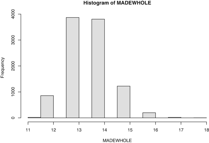

  

  Histogram of the time it takes for investors to be made whole

  MADEWHOLE<-c() for (i in 1:N){   MADEWHOLE[i]<-sum(TCPAY[i,]<f0)+1} hist(MADEWHOLE)

  Carefully notice how the MADEWHOLE data vector is created from the TCPAY matrix, by adding-up the number of entries in the row that are less than the original f0, and also make sure you understand why the number one is added. The key takeaway is that live investors are made whole (in our simulation run) somewhere between a minimum of 12 years and maximum of 16 years. More specifically, the command (sum(MADEWHOLE==13)+sum(MADEWHOLE==14))/10000 results in close to 77% of scenarios being made whole during years 13 and 14, and another 12% during the 15th year. In year 12, we see 9% are made whole. Around one quarter of one percent of scenarios had investors waiting for more than 16 years to get their money back. By then, the vast majority (who were still alive) had received at least $100,000 in dividends. Anyone who died after year 17, which would be age 82, had received their entire money back (albeit slowly over time).

• 4. Question: Focus on the GLIVE matrix and the TCPAY matrix and please use those two datasets to compute the number of original investors GL0, who when they died did not get their full money back. In other words, the sum of the tontine dividends they received until their death didn’t exceed their original investment. Remember that people who die in year i aren’t entitled to any tontine dividends in that year. Once you have figured this out, compute the number of investors who got less than 80% back, less than 60% back and less than 40%, at the time they died.

  Answer: After running the v1.0 script from the chapter, we created the following.

  SHORT<-matrix(nrow=N,ncol=5) for (i in 1:N){   SHORT[i,1]<-GL0-GLIVE[i,sum(TCPAY[i,]<100)+1]   SHORT[i,2]<-GL0-GLIVE[i,sum(TCPAY[i,]<80)+1]   SHORT[i,3]<-GL0-GLIVE[i,sum(TCPAY[i,]<60)+1]   SHORT[i,4]<-GL0-GLIVE[i,sum(TCPAY[i,]<40)+1]   SHORT[i,5]<-GL0-GLIVE[i,sum(TCPAY[i,]<150)+1]} summary(SHORT)

  Once again, the results will be simulation specific. For example, in our simulation run, somewhere between 138 investors (the minimum value in the summary) and 351 investors (the maximum value in the summary), from a total of GL0=1000 investors, died early and without getting their money back. This is between 14% and 35% of investors who at the time of death have not recovered their original investment. The first quartile was 194 investors and the 3rd quartile was 228 investors, which gives a better sense of the range (between 19% and 23%) of investors who never recover their original investment in the basic (version 1.0) tontine without any refunds or guarantees. Here is the rest of the output of the script.

  > summary(SHORT)        V1              V2              V3  Min.   :138.0   Min.   : 94.0   Min.   : 58.0  1st Qu.:194.0   1st Qu.:139.0   1st Qu.: 93.0  Median :211.0   Median :151.0   Median :100.0  Mean   :212.2   Mean   :151.3   Mean   :101.2  3rd Qu.:228.0   3rd Qu.:162.0   3rd Qu.:109.0  Max.   :351.0   Max.   :239.0   Max.   :163.0        V4              V5  Min.   : 31.0   Min.   :244.0  1st Qu.: 58.0   1st Qu.:374.0  Median : 64.0   Median :411.0  Mean   : 63.7   Mean   :417.4  3rd Qu.: 70.0   3rd Qu.:454.0  Max.   :106.0   Max.   :749.0

• 5. Question: Modify the basic simulation so dividends are paid quarterly, and generate results assuming the same Gompertz: m = 90, b = 10, and r = 4% case. Be very careful when you modify the code (and increase the size of all the matrices) that your returns and payouts are properly adjusted. For example, the 3-month survival probability and investment return is obviously quite different from the 12-month values. Once you are done, confirm the TCPAY values after 10, 20 and 30 years are virtually the same.

  Answer: The script below gives the values of a modern tontine making k payments a year, where k = 4 represents the case of quarterly dividends.

  k<-4; TH<-30; N<-10000; m<-90; b<-10; x<-65; GL0<-1000; EXR<-0.04; r<-0.04; SDR<-0.03; f0<-100; GLIVE<-matrix(nrow=N,ncol=TH*k) GDEAD<-matrix(nrow=N,ncol=TH*k) for (i in 1:N){GDEAD[i,1]<-rbinom(1,GL0,1-TPXG(x,1/k,m,b)) GLIVE[i,1]<-GL0-GDEAD[i,1] for (j in 2:(TH*k)){x1<-1-TPXG(x+(j-1)/k,1/k,m,b) GDEAD[i,j]<-rbinom(1,GLIVE[i,j-1],x1) GLIVE[i,j]<-GLIVE[i,j-1]-GDEAD[i,j]}} PORET<-matrix(nrow=N,ncol=TH*k) STPRV<-matrix(nrow=N,ncol=TH*k) for (i in 1:N){   PORET[i,]<-exp(rnorm(TH*k,EXR/k,SDR/sqrt(k)))-1}

  In the above script, for the most part we can divide parameters by the value of k, to convert them into the required frequency, other than the standard deviation of investment returns (σ) which must be divided by the square root of k. Recall that variance scales by k, but volatility is the square root of variance. Now, with the life & death matrices, as well as the investment returns in place, we can modify the TLIA function to account for k annual payments and finally calculate tontine fund values and dividends.

  TLIA<-function(x,y,r,m,b){   APV<-function(t){p2<-exp(exp((x-m)/b)*(1-exp((t/k)/b)))   exp(-r*t/k)*p2}; sum(APV(1:((y-x)*k)))} DETFV<-matrix(nrow=N,ncol=TH*k) TONDV<-matrix(nrow=N,ncol=TH*k); kappa<-c() for (i in 1:(TH*k)){kappa[i]<-1/TLIA(x+(i-1)/k,x+TH,r,m,b)} for (i in 1:N){TONDV[i,1]<-kappa[1]*f0 DETFV[i,1]<-f0*GL0*(1+PORET[i,1])-TONDV[i,1]*GLIVE[i,1] for (j in 2:(TH*k)){   TONDV[i,j]<-kappa[j]*DETFV[i,j-1]/GLIVE[i,j-1]   d3<-TONDV[i,j]*GLIVE[i,j]   DETFV[i,j]<-max(DETFV[i,j-1]*(1+PORET[i,j])-d3,0)}}

  With our basic matrices computed and in place, the final step is to create the (also much larger) TCPAY matrix and summarize its values.

  TCPAY<-matrix(nrow=N,ncol=TH*k) for (i in 1:N){TCPAY[i,]<-cumsum(TONDV[i,])} summary(TCPAY[,10*k]) summary(TCPAY[,20*k]) summary(TCPAY[,30*k])

  If you (the reader or user) have done this part correctly—and this really is the “test yourself” portion—then your TCPAY results with quarterly dividends should very closely match the original results in chapter (i.e. annual dividends) at the end of year 10, 20, 30. The small difference (if any) can be blamed on the fact that it’s a completely new simulation, but the differences should really be quite small. Here is the output we got.

  > summary(TCPAY[,10*k])    Min. 1st Qu.  Median    Mean 3rd Qu.    Max.   59.95   71.99   74.73   74.89   77.56   92.82 > summary(TCPAY[,20*k])    Min. 1st Qu.  Median    Mean 3rd Qu.    Max.   111.1   141.7   149.7   150.2   157.8   203.1 > summary(TCPAY[,30*k])    Min. 1st Qu.  Median    Mean 3rd Qu.    Max.   160.7   210.6   224.7   226.0   239.9   327.6

9.2 Chapter 4: Brief Solutions to Test Yourself Qs.

• 1. Question: Assuming that in fact nobody dies in the first decade of the tontine fund, and that mortality only kicks-in after the age of 75, please compute the number of extra survivors that this creates at the end of the TH=30 year horizon. Does this have a material impact on the number of people who survive from age x = 65 to age x = 95? Explain this intuitively.

  Answer: We ran the following script to see what happens to GLIVE[,TH] if nobody dies in the first ten years.

  #no deaths first 10 years for (i in 1:N){   GDEAD[i,1:10]<-0   GLIVE[i,1:10]<-GL0   for (j in 11:TH){     GDEAD[i,j]<-rbinom(1,GLIVE[i,j-1],1-TPXG(x+j-1,1,m,b))     GLIVE[i,j]<-GLIVE[i,j-1]-GDEAD[i,j]}}

  > summary(GLIVE[,TH])    Min. 1st Qu.  Median    Mean 3rd Qu.    Max.   194.0   231.0   240.0   240.4   249.0   294.0

  We now compare these numbers to the baseline case in the script below.

  #regular Gompertz for (i in 1:N){   GDEAD[i,1]<-rbinom(1,GL0,1-TPXG(x,1,m,b))   GLIVE[i,1]<-GL0-GDEAD[i,1]   for (j in 2:TH){     GDEAD[i,j]<-rbinom(1,GLIVE[i,j-1],1-TPXG(x+j-1,1,m,b))     GLIVE[i,j]<-GLIVE[i,j-1]-GDEAD[i,j]}}

  > summary(GLIVE[,TH])    Min. 1st Qu.  Median    Mean 3rd Qu.    Max.   160.0   200.0   209.0   208.7   217.0   257.0

  If there are no deaths in the first decade there is median value of 31 additional survivors to age 95. That is only 3% of the initial pool of 10,000 which is not very significant. The intuition here is that if we start with a large pool of 65 year old’s, and miraculously “don’t kill” any of them for a decade, the 13% of them, i.e. 1-TPXG(65,10,90,10) who were supposed to die in the first decade end-up perishing in the subsequent quarter century.

• 2. Question: Along the same lines, please compute the long-run tontine dividend value (i.e. the intercept in the regression) if the modern tontine fund was initially set-up assuming the modal value of the Gompertz parameter was m = 90, but in fact realized mortality was (much lower, and) consistent with m = 93. What is the cost in basis points (i.e. initial yield versus eventual yield)? How many more survivors will the extra 3 modal years lead to at age 95? Explain intuitively.

  Answer: To answer this question, we modified only two lines in the entire R-script, changing the realization of GDEAD to reflect the lower mortality. Here are those two lines.

  GDEAD[i,1]<-rbinom(1,GL0,1-TPXG(x,1,93,b)) GDEAD[i,j]<-rbinom(1,GLIVE[i,j-1],1-TPXG(x+j-1,1,93,b))

  In our simulation run (using set.seed(123)), the median tontine dividend drops from $7,671 in the first year to $4,597 in year 30, this is decline of over 300 basis points, from the initial yield to the final yield. The number of survivors in year 30 goes up to 314, from 209 in our baseline case. The intercept in the canonical regression increases to 8.2 (thousand) from 7.66 (thousand). The intuition here is that when realized mortality rates are lower than anticipated when the pool was set-up, dividends in the beginning are too high and must be adjusted downwards overtime as participants (to put it crudely) refuse to die as planned. The slope coefficient in the canonical regression shows a decline on average of $88 per year in tontine dividends. The volatility of tontine dividend (in this misestimated m case) increases from 13% to 17% as well. These numbers don’t really do justice to the problem, and we refer readers to a more complete discussion of model risk in Chap. 7.

• 3. Question: Going back to the canonical (standard) simulation results, with (x = 65, m = 90, b = 10), carefully examine the TONDV matrix and compute the number of scenarios in which the tontine dividend payout falls below 80% of the original payout κ ₁, at some point over the 30 year horizon. In other words, what is the probability of a 20% (or more) reduction in the cash-flow provided by the annuity, over the retirement horizon? What is the probability of (only a) a 10% or more reduction?

  Answer: We use the standard v1.0 simulation, but then add the following R-script to compute the number of scenarios in which the above-noted events take place.

  c80<-0;c90<-0 for (i in 1:N){   c80<-c80+(min(TONDV[i,])<0.8*TONDV[i,1])   c90<-c90+(min(TONDV[i,])<0.9*TONDV[i,1])} c80/N;c90/N

  The essence of the script is a counter that adds the number 1 every time the loop finds a simulation scenario in which the worst tontine dividend min(TONDV[i,]) was less than 80% (and separately 90%) of the initial tontine dividend TONDV[i,1]. After finding all those (bad) scenarios, it then scales the total by N and reports the probability, or better described as frequency. We should note that these sorts of estimates and numbers are related to extreme value statistics, a very important branch of statistics—and one that requires additional attention. The results were a 25% probability of having at least one tontine dividend below 80% of the initial payout rate, and a 56% probability of having at least one dividend below 90% of the initial payout rate.

• 4. Question: Similar to the prior question, but subtly different, what is the probability that at any point during the life of the fund the tontine dividend is reduced by 20%? Notice that this “event” is a larger subset of cases, because it also includes the situation in which tontine dividends are increased (in year 5, for example) and then reduced (in year 10, for example) so that from peak to trough the reduction was 20% or more.

  Answer: Echoing the trick used earlier, after running the standard simulation we used the following script:

  c80<-0 for (i in 1:N){   a1<-TONDV[i,1]   for (j in 1:TH){     a1<-max(a1,TONDV[i,j])     if (TONDV[i,j]<0.8*a1){c80<-c80+1; break}}} c80/N

  The resulting probability ranged from 41% to 44%. We then generated the canonical simulation using N = 100, 000 instead of N = 10, 000, and the results were consistently around 43%.

• 5. Question: Imagine that every single year the sponsor or manager extracts or removes $100,000 from the fund (per $100 million of initial fund value) to cover operating expenses. Clearly, the theoretical κ ₁ payout rate is no longer sustainable and the tontine dividends will experience a negative drift over time, as evidenced by the regression slope coefficient. Using a numerical process of trial and error, and again assuming the canonical parameter values, please locate the revised value of ${\hat {\kappa }_1}$ that will support a stable and non-declining tontine dividend over time. How many basis points of initial yield $\kappa _1-\hat {\kappa }_1$ does this annual $100,000 fixed withdrawal cost the shareholders in the fund? Are there any other issues or problems that are encountered when $100,000 is extracted every year?

  Answer: There are many ways to address this problem, each with its own embedded set of economic assumptions. One (very easy) way to model this is by computing the present value of (the fixed) $100,000 per year for 30 years, and then removing that sum from the initial value of the fund. Under an r = 4% interest rate that present value would be computed via RGOA(0,0.04,30)*100000, which is equal to $\$1,\!729,\!203$, or approximately 1.73% of the initially contributed $100 million. Another way to think about this present value is that every one of the GL0=1000 participants must give up or contribute $\$1,\!729$ from their initial investment to fund this fixed annual cost. Then, the remaining $\$98,\!271$ goes into a fee-free tontine fund that yields the usual κ ₁ = 7.67%, or 0.0767 × 98271 for a dividend of $7, 538. That, for the record, is 13 basis points less in κ yield. The fund then promises the (revised) tontine dividend, removes the PV of the fixed fees up-front (perhaps in a separate bank account) and the payouts will be stable, albeit from a slightly smaller fund. Now, whether extracting $1.73 million from the decumulation tontine fund at time zero will be viewed as equivalent to removing $100 thousand per year by the regulators and shareholders is a completely separate matter.

9.3 Chapter 5: Brief Solutions to Test Yourself Qs.

• 1. Question: Please generate a tontine dividend dashboard in which the initial seed is changed from (the year) 1693 to 3961. Discuss how (all) the results change, and why.

  Answer: We generated results using the v2.0 script after running set.seed(3961), then continued with the following scripts and finally copied the results to the table (Table 9.3).

  Table 9.3 Tontine dashboard: dividend distribution; replicate with set.seed(3961)

  temp<-matrix(nrow=6,ncol=5) n1<-0 for (j in c(.01,.25,.5,.75,.99)){   n1<-n1+1   n2<-0   for (i in c(1,5,10,20,30)){     n2<-n2+1     temp[n1,n2]<-quantile(TONDV[,i],j)*1000     temp[6,n2]<-sd(TONDV[,i])*1000   }} temp

  Here are the results:

  The results will change whenever R generates new and different numbers randomly. This affects the number of survivors each year as well as the investment returns, which in turn impact the dividend payout, as one might expect.

• 2. Question: Please create, report and display a tontine dashboard (similar to Table 5.1), but for the aggregate amount of death benefits paid to those who die in the years T = 1, 5, 10, 15, 20. That is the AGDEB[i,j] matrix. Explain qualitatively what happens in the later (year’s) columns and discuss the statistical distribution of those death benefit payouts. Do they seem normally distributed around the mean value? Discuss.

  Answer: We ran the v2.0 script using the 1693 seed, then the following script and finally copied the results to the table (Table 9.4).

  Table 9.4 Tontine dashboard: aggregate death benefits; replicate with set.seed(1693)

  temp<-matrix(nrow=6,ncol=5) n1<-0 for (j in c(.01,.25,.5,.75,.99)){   n1<-n1+1   n2<-0   for (i in c(1,5,10,15,20)){     n2<-n2+1     temp[n1,n2]<-quantile(AGDEB[,i],j)*1000     temp[6,n2]<-sd(AGDEB[,i])*1000   }} temp

  Here are our results:

  In year 15 more than a quarter of the simulations have already paid out $100,000 in dividends, so their aggregate death benefit is zero that year. In year 20, virtually all of the simulated cases have exceeded $100,000 in total dividends paid to the living investors, so no one who dies that year would be entitled to a death benefit. In years 10 and 15 the distribution seems to have a long right tail. The 75th percentile is much farther from the median than the 25th percentile. This is clearly not normally distributed. Readers may also have noticed that (strangely) the standard deviation in year 20 is not zero. This is because there are 5 scenarios out of the 10,000 in which there are still death benefits paid out even in the 20th year. You can test this yourself by running sum(AGDEB[,20]>0).

• 3. Question: Assume that a (nefarious or misguided) tontine sponsor claims they will offer a death reimbursement covenant, but instead decides to pay the beneficiaries of the deceased a tontine dividend until the entire $f_0:=\$100,\!000$ is returned to the heirs. The death benefit is stretched out over time, instead of being paid out at once. They say: Don’t worry, we will make your family whole again, but slowly… Please modify the core simulation v2.0 to account for this feature, discuss whether it makes any difference at all on the tontine dividend payouts, and carefully explain your results.

  Answer: We modify the TLIA_RDB function in order to reflect the fact that the death benefit is not RDB but rather an annual payment whose sum equals RDB. This is one possible way of solving this problem. Another would be to break the valuation (and κ function) in two parts, one a term certain annuity, and the other a deferred annuity. Either way the answer will look something like this.

  TLIA_RDB<-function(x,y,r,m,b,RDB){   periods<-(y-x)   value<-0   for(i in 1:periods){     PV<-exp(-r*i)     # The next 3 lines should be combined as one     value<-value+TPXG(x,i,m,b)     *PV+(sum((1+r)^-(0:(max(RDB-(i-1),0))))-1)     *TQXG(x,(i-1),i,m,b)*PV}   value}

  We also adjust the AGDEB matrix to reflect the dividends paid to those who are dead instead of the lump sum. Again, we emphasize this isn’t the only way to solve this particular problem.

  for (i in 1:N){   TONDV[i,1]<-kappa[1]*f0   TCPAY[i,1]<-TONDV[i,1]   # Define aggregate death benefits paid (for fund)   AGDEB[i,1]<-TONDV[i,1]*GDEAD[i,1]   outflow<-TONDV[i,1]*GLIVE[i,1]+AGDEB[i,1]   DETFV[i,1]<-f0*GL0*(1+PORET[i,1])-outflow   for (j in 2:TH){     if (GLIVE[i,j]>0){       TONDV[i,j]<-kappa[j]*DETFV[i,j-1]/GLIVE[i,j-1]}     else {TONDV[i,j]<-0}     TCPAY[i,j]<-TCPAY[i,j-1]+TONDV[i,j]     # Define aggregate death benefits paid (for fund)     if (TCPAY[i,j-1]<f0){       AGDEB[i,j]<-TONDV[i,j]*(GL0-GLIVE[i,j])}     else {AGDEB[i,j]<-0}     outflow<-TONDV[i,j]*GLIVE[i,j]+AGDEB[i,j]     DETFV[i,j]<-DETFV[i,j-1]*(1+PORET[i,j])-outflow}}

  The initial tontine dividend payout is approximately $7,244 per year, which is somewhere between the $7,074 number with a normal death benefit, and the $7,671 with no death benefit. This is intuitive, because the present value of the death benefit is lower than the canonical v2.0, but still greater than zero, which is the v1.0 scenario. These results were obtained using the 1693 seed. The resulting dividends appear to have a small (around $37 per year) negative slope over time, which is worth thinking about more carefully.

• 4. Question: Please generate simulation results and create a table similar to the canonical dashboard, in which the reimbursement covenant is weakened in the following manner. If at the end of the year the aggregate value of the decumulation tontine fund is less than the original investment minus dividends received, those who died during that year receive the lower of the two values. So, for example, consider the following scenario. Tontine dividends of exactly $7, 000 are received for 3 years, and in the 4th year the investor dies. Under the normal covenant, the beneficiaries of the deceased should receive a death benefit of $100, 000 minus the $21, 000 already received, which is: $79, 000 at the end of year 4. But imagine that the total fund value happens to only be worth $60 million, perhaps due to a (very) bad year in the markets, and there are 800 survivors at the end of year #4. This implies that the notional value of the fund at the end of the 4th year is $\$75,\!000$ per live survivor. One can think of this as the reserve per person. But, this is also $4, 000 less than the death benefit promised under a strong covenant. Well then, under the weak one proposed here, it would be reduced to $\$75,\!000$. Obviously this situation is somewhat artificial, but nevertheless please generate dashboard results under this particular design and report the distribution of the number of people—from an original pool of 1000 investors—who die and do not get their entire money back. Discuss the qualitative impact of fund values and tontine dividends, when initially RTLIA is used to set payouts but then weakened when someone actually dies.

  Answer: We changed the v2.0 script to calculate AGDEB based on the so-called weak covenant and added a counter to measure how many times the weak covenant actually affects the death benefit. Here is the script.

  count <- c() for (i in 1:N){   count[i]<-0   TONDV[i,1]<-kappa[1]*f0   TCPAY[i,1]<-TONDV[i,1]   AGDEB[i,1]<-GDEAD[i,1]*min(f0,f0*(1+PORET[i,1]))   # The next two lines should be combined.   DETFV[i,1]<-f0*GL0*(1+PORET[i,1])-TONDV[i,1]   *GLIVE[i,1]-AGDEB[i,1]   for (j in 2:TH){     TONDV[i,j]<-kappa[j]*DETFV[i,j-1]/GLIVE[i,j-1]     TCPAY[i,j]<-TCPAY[i,j-1]+TONDV[i,j]     # The next two lines should be combined.     AGDEB[i,j]<-max(min(f0-TCPAY[i,j-1],DETFV[i,j-1]                 *(1+PORET[i,j])/GLIVE[i,j]),0)*GDEAD[i,j]     # The next two lines should be combined.     DETFV[i,j]<-DETFV[i,j-1]*(1+PORET[i,j])-TONDV[i,j]     *GLIVE[i,j]-AGDEB[i,j]     # The next two lines should be combined     if (f0-TCPAY[i,j-1]>DETFV[i,j-1]         *(1+PORET[i,j])/GLIVE[i,j])     {count[i]<-count[i]+GDEAD[i,j]}   }}

  The weak covenant does not affect the dividend payout, which sits around $7,084 as the intercept in the regression model. The slope of the regression is roughly 0, and this was when the 1693 seed was used (Table 9.5).

  Table 9.5 Tontine dashboard: dividend distribution under Weakened covenant; replicate with set.seed(1693)

  It appears there is no meaningful change in the tontine dividend payout if the covenant is weakened. This is also evident from the distribution of the number of investors who die without getting their money back which is quite rare in our scenarios. We created a frequency table of our count vector, which measures how many people died in each simulation without getting their money back. It appears that in 98% of simulations, no investors died without getting their money back. Qualitatively, the weak covenant makes no difference to the evolution of the fund value compared to the strong covenant, but the latter certainly sounds better than the former.

  > table(count) count    0  1  2  3  4  5  6  7  8  9 10 11 9809  1  1  3  6  9 14 20 14 20 17 14   12 13 14 15 16 17 18 19 20 21 22 23   11  5  7  1  2  3  3  5  6  5  4  1   24 25 26 27 29 30 32 36 41 45 46 50    3  1  2  3  2  1  1  1  1  1  1  1   56    1

• 5. Question: Modify the v3 script to allow new members to join the tontine in the first 15 years. You can do this by adding LAPSE to our GLIVE values (instead of subtracting LAPSE). When a new person joins during the first 15 years, they pay a lower f0 into the fund, their initial investment is reduced by 30% of TCPAY ( 30% of the dividends they missed out on by joining late). After 15 years we no longer allow people to join. Also note that we do not allow people to lapse in this specific fund. Find the median tontine dividend for this fund.

  Answer: Using the same 1693 seed, we modify the v3.0 script as follows. First we set dsc<-0.3 instead of dsc<-0.25. Next we modify the part of the script that computes GLIVE to add those that join (negative lapsers), and then we assume eta=0.02 for the first 15 years.

  for (i in 1:N){   LAPSE[i,1]<-rbinom(1,GL0,eta[1])   GDEAD[i,1]<-rbinom(1,GL0,1-TPXG(x,1,m,b))   GLIVE[i,1]<-GL0-GDEAD[i,1]+LAPSE[i,1]   for (j in 2:TH){     LAPSE[i,j]<-rbinom(1,GLIVE[i,j-1],eta[j])     GDEAD[i,j]<-rbinom(1,GLIVE[i,j-1],1-TPXG(x+j-1,1,m,b))     GLIVE[i,j]<-GLIVE[i,j-1]-GDEAD[i,j]+LAPSE[i,j]}}

  Note that we must change AGLAP to calculate the aggregate amount contributed to the fund by new joiners, and we must modify outflow by subtracting AGLAP instead of adding it.

  for (i in 1:N){   TONDV[i,1]<-kappa[1]*f0   TCPAY[i,1]<-TONDV[i,1]   AGDEB[i,1]<-f0*GDEAD[i,1]   AGLAP[i,1]<-(f0-TCPAY[i,1]*dsc)*LAPSE[i,1]   outflow<-TONDV[i,1]*GLIVE[i,1]+AGDEB[i,1]-AGLAP[i,1]   DETFV[i,1]<-f0*GL0*(1+PORET[i,1])-outflow   for (j in 2:TH){     TONDV[i,j]<-kappa[j]*DETFV[i,j-1]/GLIVE[i,j-1]     TCPAY[i,j]<-TCPAY[i,j-1]+TONDV[i,j]     AGDEB[i,j]<-max(f0-TCPAY[i,j-1],0)*GDEAD[i,j]     AGLAP[i,j]<-max(f0-TCPAY[i,j-1]*dsc,0)*LAPSE[i,j]     outflow<-TONDV[i,j]*GLIVE[i,j]+AGDEB[i,j]-AGLAP[i,j]     DETFV[i,j]<-DETFV[i,j-1]*(1+PORET[i,j])-outflow}}

  The median dividend in the 20th year is $7,176, which is higher than the baseline case. The objective of this question is to get you to start thinking about how we would deal with new people joining the tontine after it already started.

9.4 Chapter 6: Brief Solutions to Test Yourself Qs.

• 1. Question: Please generate a PORET[i,j] matrix in which 40% of the tontine fund assets are placed in a fund resembling the historical SP500 total return index, and the remaining 60% of the fund is invested in fixed income bonds that are normally distributed with a mean return of 2%, and volatility of 4%, per annum. There is no need to generate the entire modern tontine simulation, but please report the summary mean, standard deviation, skewness and kurtosis of the PORET[i,j] matrix in the tenth year of the fund.

  Answer: The following script illustrates how to create this mixed PORET matrix and gives the first four moments of PORET in the tenth year of the fund.

  set.seed(1693) for (i in 1:N){   # The next two lines should be combined.   PORET[i,]<-0.6*rnorm(TH,0.02,0.04)   +0.4*ANPATH(SP500TR$RETURN,TH)} mean(log(1+PORET[,10])) > 0.05631358 sd(log(1+PORET[,10])) > 0.06735162 skewness(log(1+PORET[,10])) > -0.003604842 kurtosis(log(1+PORET[,10])) > 3.020791

  This type of allocation provides moments that constitute an average of the volatile high-return SP500 and the more stable low-return bond fund. The skewness and kurtosis of this mixture is close to that of LogNormal.

• 2. Question: Create a PORET[i,j] matrix in which investment returns are based entirely on the historical SP500 total return, but the annual returns are both floored and capped. The floor and cap are located at the upper and lower 15th percentile. What this means is that 15% of the worst months are not used or experienced by the fund, in exchange for giving up or sacrificing the 15% of best months. To be very clear, your bootstrap procedure should only use 100% or all of 612 months, but replace the extreme returns with their floored and capped values. Again, there is no need to simulate tontine dividends. Rather, report the summary statistics (a.k.a. moments) of this PORET[i,j] matrix in the 10th year.

  Answer: The following script illustrates how to bootstrap the capped & floored PORET matrix and returns the first four moments of PORET in the tenth year of the fund.

  set.seed(1693) PORET<-matrix(nrow=N,ncol=TH) for (i in 1:N){ # Sample SP500   P1<-ANPATH(SP500TR$RETURN,TH) # Replace bottom 15\% with floor   P1[P1<quantile(P1,0.15)]<-quantile(P1,0.15) # Replace top 15\% with cap   P1[P1>quantile(P1,0.85)]<-quantile(P1,0.85)   PORET[i,]<-P1} mean(log(1+PORET[,10])) > 0.1042289 sd(log(1+PORET[,10])) > 0.1127769 skewness(log(1+PORET[,10])) > -0.07229733 kurtosis(log(1+PORET[,10])) > 1.991791

  It looks like the caps & floors significantly reduce the volatility of returns from 15% to 11% without reducing the mean. The skewness here is -0.07 which is not as bad as the -0.20 of the uncapped returns, and the kurtosis is 1.99, which is also quite a bit lower than the 3.2 of the uncapped case. From this simulation it appears that caps and floors are a highly effective way to reduce the modern tontine’s fund volatility over time.

• 3. Question: The discussion of skewness and kurtosis has been devoted exclusively to the investment returns, but the same computation and summary statistics could be applied to the tontine dividends. Please generate the numbers underlying Tables 6.1 and 6.2 and compare the skewness and kurtosis of the modern tontine dividends in the 10th year of the fund. Note that the 10th year is rather arbitrary, but a horizon or time period must be fixed whenever the summary statistics are computed. Averaging all of the dividends or all of the returns would be mixing too many (calendar) apples and oranges.

  Answer: After running the v2.0 tontine script using the two different PORET matrices, one bootstrapped from the SP500 index and the other LogNormally generated with EXR=0.1 and SDR=0.15. In both cases we used the 1693 seed. When we used the LogNormal distribution the skewness of the dividends in the tenth year was 1.71 and kurtosis was 8.28. When we bootstrapped from SP500 the skewness of the dividends in the tenth year was 1.64 and kurtosis was 7.64. Overall the skewness and kurtosis of PORET do not have a substantial impact on the skewness and kurtosis of the tontine dividends, which are naturally very high.

• 4. Question: The previous question explored the effect that skewness and kurtosis of the PORET matrix have on the skewness and kurtosis of TONDV[,10]. This question looks at how PORET volatility affects the skewness and kurtosis of TONDV[,10]. Generate a PORET matrix where volatility is 0, and the expected annual return and discount rate are 10%. Use this returns matrix to simulate modern tontine dividends and measure the skewness and kurtosis of the dividends in the 10th year.

  Answer: We ran the v2.0 script using EXR<-0.1; SDR<-0; r<-0.1; and then measured skewness(TONDV[,10]) and kurtosis(TONDV [,10]). The skewness was 0.2 and the kurtosis was 3.2. It appears that the high skewness and kurtosis of the tontine dividends are primarily caused by the volatility of the portfolio returns. We also reran this experiment with various seeds, and much higher values for GL0, N and b, the skewness and kurtosis were consistently around 0 and 3, respectively.

9.5 Chapter 7: Brief Solutions to Test Yourself Qs.

• 1. Question: Using the non-tontine natural decumulation fund, please generate a table with the median as well as the (top) 99th and (bottom) 1st percentile of the fund value in 5, 10, 15 and 20 years, assuming a 4% expected return and valuation rate, and a 3% standard deviation, for a 30 year time horizon. Compare with the results for a modern tontine (version 1.0) and confirm that the volatility of the payouts (a.k.a. dividends) as a percent of the expected value is indeed higher for the tontine fund. Finally, force the m parameter to be (astronomically) high for the modern tontine script and confirm you get the same exact numerical results as the natural decumulation fund (Tables 9.6 and 9.7).

  Table 9.6 Natural decumulation fund dividend distribution; replicate with set.seed(1693)

  Table 9.7 Modern tontine dividend distribution; replicate with set.seed(1693)

  Answer: The volatility of payouts in year 20 is 14% for the natural decumulation fund and 15% for the modern tontine. We forced the m parameter to be nine million (yes, years) and generated the standard tontine v1.0 script. Here are our results (Table 9.8):

  Table 9.8 Modern tontine with m = 9 million that mirrors natural decumulation fund; replicate with set.seed(1693)

  It appears the volatility of payouts is also 14%, just like the natural decumulation fund. Our dividend values are also statistically the same as those of the natural decumulation fund, but the numbers are slightly different even though we use the same 1693 seed. The small difference is caused by the fact the modern tontine algorithm generates (some, redundant) random numbers for the GDEAD matrix before it generates the random numbers for the PORET matrix. Even though all the GDEAD numbers are zero, due to the astronomically high m value. The random number generator is still affected by this step, so we get the result of (basically) using a different seed.

• 2. Question: Although the pattern of dividends or better described as payouts for the natural decumulation fund was presented within the chapter, please generate the relevant figures for the underlying fund value (using the same parameter values) and then discuss and explain their qualitative pattern.

  Answer: Figure 9.2 shows the dividends and Fig. 9.3 shows the fund value of the natural decumulation fund over time. For this fund, dividends are lower and less volatile than for the modern tontine. The fund’s value over time appears to be more concave as opposed to a modern tontine which seems more convex. In the beginning, when death is rare, the natural decumulation fund value declines slower than a modern tontine since it pays individual investors a smaller dividend. Towards the end, when many people have died, the natural decumulation fund value declines quicker than the modern tontine since it needs to pay dividends to GL0 investors, while the modern tontine only pays dividends to those who survive.

  Fig. 9.2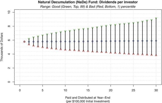

  

  Natural Decumulation (NaDe) fund dividends

  Fig. 9.3

  

  Natural Decumulation (NaDe) fund value

• 3. Question: Investigate the impact of getting the dispersion coefficient (b) wrong, like we did for the modal value coefficient (m). In particular, assume some reasonable investment returns and that (m = 90, b = 10) for pricing purposes, but that realized mortality is such that b = 7. In other words, the dispersion of lifetimes is lower, and the rate at which mortality accelerates 1∕b is higher than 10%. What is the qualitative impact on the pattern of modern tontine dividends over time?

  Answer: If the dispersion coefficient is 7 but we pay dividends assuming b = 10 then the dividends will trend downwards for the first 18 years and then they will begin trending upwards quickly. Here is the intuition behind this, in the first 18 years, before investors are: m − b or 90 − 7 = 83 year old, fewer people die each year than expected so the dividends fall. After year 18, we get more deaths each year than what we expected, since the deaths are more closely clustered around m. After time m, the number of survivors drops quicker than expected, so dividends keep rising. If we assume b = 7 and the dispersion coefficient is indeed 7, then the dividends will be stable around 7.4 which is lower than our baseline case. Overall the higher and larger the dispersion coefficient b, the greater the tontine dividends, all else remaining equal. Why? Well, life expectancy will be lower, which then increases the mortality credits. Here are the median annual dividends in the baseline case when we assume correctly that b = 10:

   [1] 7671 7671 7666 7667 7674 7664 7665 7661 7666 7666 7668 [12] 7661 7664 7658 7661 7661 7673 7662 7666 7672 7662 7662 [23] 7664 7664 7652 7653 7633 7636 7642 7626

  And, here they are when we (also) assume b = 10 but it turns out to be 7. Notice the fall and then rise.

   [1] 7671  7635  7594 7551  7510 7478 7428  7376 7331 [10] 7285  7235  7186 7154  7108 7071 7056  7040 7029 [19] 7043  7082  7134 7225  7365 7575 7863  8257 8845 [28] 9669 10922 13275

  Finally, here is what happens if we assume correctly that b = 7.

   [1] 7444 7444 7441 7438 7437 7448 7442 7435 7436 7436 7431 [12] 7424 7434 7426 7421 7430 7431 7421 7421 7423 7415 7409 [23] 7400 7404 7408 7400 7422 7426 7418 7395

• 4. Question: Use the (magic) script to locate the best fitting (m, b) parameters for the basic CPM2014 mortality table at age 65, and then compute the initial payout yield using the Gompertz TLIA(.) function under a 4% and 2% valuation rate assumption. Compare that to the 7.4% and 6.0% yields derived and explained in the chapter.

  Answer: We ran the following script after loading the (static) mortality table CPM2014.

  qx<-CPM2014$qx_u[48:77] x<-65:94; y<-log(log(1/(1-qx))) fit<-lm(y~x) h<-as.numeric(fit$coefficients[1]) g<-as.numeric(fit$coefficients[2]) m<- log(g)/g-h/g; b<- 1/g; m;b; > 89.8461 > 8.228034 x<-65; TH<-30 1/TLIA(x,x+TH,0.04,m,b) > 0.07529409 1/TLIA(x,x+TH,0.02,m,b) > 0.06124139

  Our numerical results were 11 basis points higher than the previously mentioned 7.42% and 6.01% yields which were derived in the chapter. This is extremely close. Remember, it is quite expected for the numbers to slightly differ since we are fitting a curve to (discrete) real world data.

9.6 Chapter 8: Brief Solutions to Test Yourself Qs.

• 1. Question: Show that adding caps do not have any material impact on the ruin probability, assuming a 4% floor.

  Answer: We look at the probability of ruin (failure) by the end of year 25 assuming a 4% floor, and see how that changes if we add an 8% cap. With no cap the ruin probability is 6.42%. But, when we add the 8% cap, the ruin probability stays the exact same. If we add a 7% cap, which is quite low, then the ruin probability drops to 6.41% which is negligible. The intuition here is that in simulated scenarios where the floor induces ruin or financial failure, the tontine dividend virtually never rises high enough to hit the cap. We used the following base parameters:

  # Base parameters are set. x<-65; m<-90; b<-10; GL0<-1000; TH<-30; N<-10000 EXR<-0.035; SDR<-0.07; r<-0.035; f0<-100; # Parameters that Govern lapsation and redemption. eta0<- rep(0.02,15) eta<-c(eta0,rep(0,TH-length(eta0))); dsc<-0.03 # Paramters that govern floors and caps kfloor<-0.04; kcap<-0.08

  To account for the cap, we modify the calculation of the tontine dividends TONDV, so that it’s generated in the following manner:

  TONDV[i,j]<-min(kappa[j]*DETFV[i,j-1]/GLIVE[i,j-1],kcap*f0) TONDV[i,j]<-max(TONDV[i,j],kfloor*f0)

• 2. Question: Show that skimming 100 basis points from the natural tontine dividend helps reduce the ruin probability or the failure rate.

  Answer: We create and set our parameters as in the previous question, but instead of kcap we create kskim<-0.01, and then we adjust the process for calculating TONDV as follows.

  # Define first dividend (per individual). TONDV[i,1]<-kappa[1]*f0-kskim*f0

  # Define annual dividend (per individual). TONDV[i,j]<-kappa[j]*DETFV[i,j-1]/GLIVE[i,j-1] TONDV[i,j]<-TONDV[i,j]-kskim*f0 TONDV[i,j]<-max(TONDV[i,j],kfloor*f0)

  When we skim 100 basis points of f0 from each annual dividend, the ruin probability by year 25 drops from 6.42% to 3.65%. This is a significant decline in the risk, but is still unacceptably high. Investors pay the price of $1,000 each year (per $100k investment) which is also very high. Overall this does not seem like a good strategy or a way of generating (more) stability.

• 3. Question: Show that skimming 100 basis points from the natural tontine dividend only during the first 10 years helps reduce the ruin probability.

  Answer: We modify the script that calculates TONDV as follows:

  TONDV[i,1]<-kappa[1]*f0-kskim*f0

  TONDV[i,j]<-kappa[j]*DETFV[i,j-1]/GLIVE[i,j-1] if (j<11){TONDV[i,j]<-TONDV[i,j]-kskim*f0} TONDV[i,j]<-max(TONDV[i,j],kfloor*f0)

  This results is ruin4[25]=0.0445 which is pretty close to the improvement or benefit generated when dividends were skimmed over the full 30 years. But now the total amount skimmed is much smaller. The message is that if we choose to skim, we only need to do that early on, and the skimming in later years is less effective.

• 4. Question: Show that skimming 100 basis points from the natural tontine dividend during years when the market return is below 0, helps reduce the ruin probability.

  Answer: We modify the script that calculates TONDV as follows:

  TONDV[i,j]<-kappa[j]*DETFV[i,j-1]/GLIVE[i,j-1] if (PORET[i,j]<0){ TONDV[i,j]<-TONDV[i,j]-kskim*f0} TONDV[i,j]<-max(TONDV[i,j],kfloor*f0)

  The result is a 4.73% ruin probability by year 25, which is not as good as when we skim every year, or when we skim for the first ten years, but the total cost is lower for most investors. We can expect to see negative market returns roughly 10 out of 30 years (sum(PORET<0)/300000), which at first glance looks like the previous scenario (when we skimmed the first 10 years). The main difference is that in this scenario most investors experience fewer skimmed years, since the probability of dividends getting skimmed is spread equally over the whole time horizon, including the later years when many investors are dead. But in the previous question most investors will be alive to have their dividend skimmed for the full 10 years. And yes, the word skim doesn’t sound very appetizing or ethical, but hopefully the mathematical point is clear.