Solving Models Using Excel

Abstract

This chapter offers examples illustrating how the ‘Solver’ feature of Excel can be used to solve simultaneous equations and unconstrained and constrained optimization models. This and other features of Excel can be used to solve any of the optimization or simulation models or equations introduced in this book.

6.1 Introduction

Recall the model developed in Chap. 3 for finding the dimensions of a tank that minimized its cost, or the model introduced in Chap. 4 for estimating the most beneficial way of allocating scarce resources to multiple users. In each case, there were multiple possible solutions, and the best solution was not obvious. These situations motivate the development of optimization models but the models themselves are of little value unless they can be solved. This book introduces ways of developing and solving optimization models. Each method has its advantages and limitations, as was evident for the hill climbing approach presented in Chap. 4. This chapter shows how optimization models can be solved using ‘Solver’ contained in the Microsoft spreadsheet program Excel.

Software programs such as Excel change over time. Hence, what is described in this chapter is only an outline of what is needed to be able to use Solver and take advantage of other capabilities of Excel when solving optimization models. It reflects the version of Excel available when this book was written. This chapter is not a substitute for the documents available from Microsoft and others that explain Excel’s features in more detail.

6.2 Using Solver in Excel

To use Excel to solve optimization problems, we need to use ‘solver’. If it is not already available under the Data menu item, it must be installed. To do this, find and click on ‘Options’ under ‘File’. Then find and click on ‘Add ins’. Then find and click on ‘Solver Add in’. Once this ‘Solver Add in’ line is highlighted, click on ‘Go’ at the bottom of the page. The following dialog box will appear. As shown below, click on the box next to ‘Solver Add-in’ and then ‘OK’. Then you can go to the ‘Data’ page of Excel, and you should see ‘Solver’ at the far right of the top row of menu items (Fig. 6.1).

Fig. 6.1

Dialog box used to select Solver to be installed in Excel

The following examples are used to illustrate how the optimization component in Excel works.

• 1. Benefit–cost analysis:

Assume a decision variable x can range between 0 and 12. Any value of x will yield benefits and incur a cost. The benefit function for this decision variable is 80x^0.55. Its cost function is 7 + 4x^1.5. Given these functions as shown in Fig. 6.2, the optimization problem is to determine the value of x that maximizes the benefits less the costs, i.e., the net benefits.

Fig. 6.2

Benefit and cost functions together with the net benefit function

Before entering this optimization model into Excel, we can also include equations that define the slopes of the benefit and cost functions associated with any value of x. As one can see from Fig. 6.2, when the net benefits are at their maximum value, the slopes of the benefit and cost functions are equal. We can use Excel to not only find the best value of x, but also verify that at that value, the marginal benefits equal the marginal costs, i.e., the slopes are the same.

Using calculus, which will be described later in Chap. 10, we can find the equations that define the marginal values or slopes of these benefit and cost functions at any value of x.

$$\begin{aligned} &{\text{marginal}}\,{\text{benefit}} = (0.55)(80)x^{(0.55 - 1)} \hfill \\ &{\text{marginal}}\,{\text{cost}} = (1.5)(4)x^{(1.5 - 1)} . \hfill \\ \end{aligned}$$

Next, we can set up the model in Excel: Fig. 6.3 illustrates one way to do this.

Fig. 6.3

Model for finding Net Benefits entered into an Excel spreadsheet

Once the model is entered into the Excel spreadsheet, we can find the optimum (maximum net benefit) solution by clicking on the Solver menu item, which again is among the menus found under the Data menu. The dialog box shown in Fig. 6.4 will appear.

Fig. 6.4

Dialog box for identifying the type of optimization, the function to be maximized or minimized or for just finding any solution, the unknown decision variables in the model, the method used for optimization, and the constraints, if any

In this example, the cell containing the objective function is F5. It is to be maximized. The value of the decision variable x is in cell E6. There are no constraints. The non-linear solver is to be used to find the best solution since the model is non-linear. Solver assumes that all unknown variables are non-negative unless otherwise specified in the constraint section.

Clicking on Solve (having the blue border in Fig. 6.4) results in the solution shown in Fig. 6.5.

Fig. 6.5

Solution of Benefit–Cost model in which the net benefits, cell F5, is a maximum

Note that the net benefits are a maximum when x is 8.144. At this x value, the slopes of the benefit and cost functions are the same, namely 17.123. Knowing that this condition will always apply, unless constrained otherwise, the value of x could have been obtained by simply equating the marginal values and solving for x. This would require adding the constraint that equates the two marginal values, as illustrated in Fig. 6.6.

Fig. 6.6

Solving the benefit–cost model by simply equating the marginal benefits and costs. This requires the constraint shown in the constraint section of this dialog box

Clicking on Solve in the dialog box shown in Fig. 6.6 will result in the same output as shown in Fig. 6.5.

• 2. Designing a cylindrical tank.

This second example involves determining the least-cost dimensions of a cylindrical tank. The design variables are the radius and the height. The known parameters are the unit (per unit area) costs of the side area, the top area, the bottom area, the required volume, and the constant pi (π).

This optimization problem has a constraint requiring the volume to be at least equal to 100 units.

Figure 6.7 shows the Excel model and the steps needed to define the objective, the decision variables, and the constraint. It also shows how to get the sensitivity information related to the constraint, called the Lagrange Multiplier. Its value indicates the additional cost if the volume were increased by one unit (i.e., the slope of the total cost function at the optimal value of the radius and height). It is also called the shadow price or dual variable as discussed in Chap. 4.

Fig. 6.7

Setting up and solving for the least-cost values of the radius and height of a circular tank

The first step is to define the model variables, and parameters, and functions in any way that makes it clear where their values will be shown. This is shown in the upper-left portion of Fig. 6.7, except in this case, where the values shown are the ones obtained after the solution is known. When setting up the model, most of the values of the decision variables and functions will be 0.

Once the model is complete, select Solver and fill in the dialog box as shown in the upper right of Fig. 6.7. To add a constraint, select the ‘Add’ button in the constraint section of the dialog box and another dialog box will appear as shown just under the model. After entering the constraint, clicking on OK will make that constraint appear in the larger dialog box as shown above. Clicking on ‘Solve’, if there are no errors, will result in the dialog box shown at the bottom right of the figure. Selecting ‘Sensitivity’ (as shown in blue) will generate the report shown at the bottom left of the figure. That report will be on a separate page of the Excel file. This option will be demonstrated in the next example problem.

• 3. Resource allocation.

This example problem is to find the allocations X, Y, and Z to three users that maximize the total benefits obtained, given only 6 units of resource available. The benefit functions for each use are:

$$B1 = 6*X - X^{2} ;B2 = 7*Y - 1.5*Y^{2} ;B3 = 8*Z - 0.5*Z^{2} .$$

The objective is to maximize B1 + B2 + B3

$${\text{Subject to}}{:}\, X \, + \, Y \, + \, Z \le {6}.$$

This is the same problem that was used to illustrate the hill climbing approach in Chap. 4 for solving models that contain continuous concave objective functions for maximization, or convex functions for minimization. Here we use Excel to solve the same model. In this case, we can assume each allocation is a continuous variable, rather than a discrete variable as was assumed for hill climbing (Figs. 6.8 and 6.9).

Fig. 6.8

The resource allocation problem is set up for solution using Solver in Excel

Fig. 6.9

Solution of the resource allocation problem, and dialog box used to access the solution shown on left and sensitivity reports shown in Fig. 6.10

Fig. 6.10

Sensitivity report associated with the resource allocation model

6.3 Conclusion

This chapter and its examples serve just as an introduction to using the Solver within Excel to find solutions to simultaneous equations or to constrained or unconstrained optimization problems. There is much more to learn besides what has been demonstrated here, and some of these additional features will be covered as we work through various policy problems introduced in the following chapters.

Relying on a computer to solve problems does not eliminate the need to think. Steve Jobs suggests programming a computer, and we assume that may also apply to using Excel, helps us think.

“Everybody in this country should learn to program a computer… because it teaches you how to think”.

Steve Jobs, co-founder and CEO of Apple, Inc. (1995–2011)

Exercises

• 1. Regression involves finding functions that best fit some observed data. One criterion is to minimize the sum of squared deviations from observed and predicted values. Suppose you have a set of observed (known) x, y values, say x(i) and corresponding y(i).

  $$\begin{array}{*{20}l} {{\text{y}}\left( {\text{i}} \right){:}} & {4} & {{1}0} & {{18}} & {{11}} & {{22}} & {7} & {{1}0} & {{14}} & {{19}} & {3} \\ {{\text{x}}\left( {\text{i}} \right){:}} & {2} & {4} & {8} & {6} & {{1}0 } & {3} & {5} & {7} & {9} & {1} \\ \end{array}$$

  Define and solve an optimization model to determine the parameters of a non-linear function y = a + bx^c that best fit the above data.

  

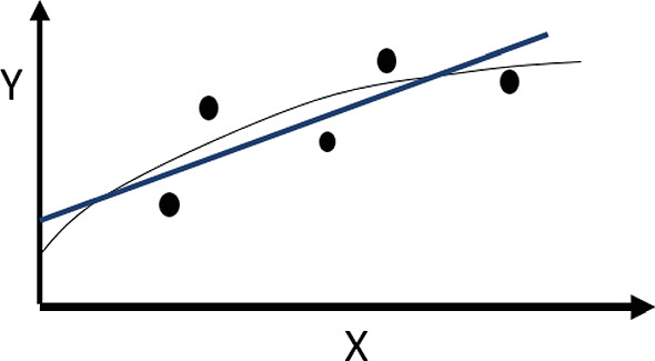
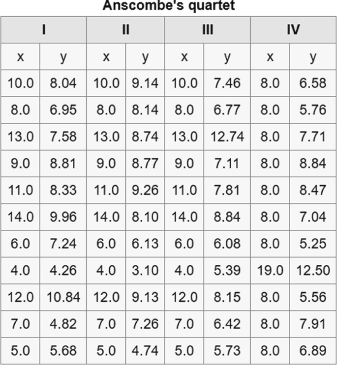
• 2. Find the four linear functions that best fit the following four sets of data. Then plot the data. What does this tell you about fitting functions to data?