Distributed Control for Conservation Laws

Abstract

This chapter focuses on control of systems of conservation laws with distributed parameters. Problem with different parameterized fluxes is addressed: in particular, we deal with cases where the control is the maximal speed and look for continuous dependence of the solution on parameters.

4.1 Introduction

This chapter focuses on control of systems of conservation laws with distributed parameters. Problem with different parameterized fluxes is addressed: in particular, we deal with cases where the control is the maximal speed and look for continuous dependence of the solution on parameters. Various examples of conservation laws with distributed control are presented. The control, in this case, acts on the flux or on the parameters of the flux, as for example the maximal speed.

In Sect. 4.2, we introduce the classical notions of Riemann Solver Semigroup solutions [51] and its stability [39].

Subsequently, in Sect. 4.3, we consider the case of variable speed limit computed via needle-like variation methods. Specifically, an optimal control problem for traffic flow on a single road using a variable speed limit is studied. The control variable is the maximal allowed velocity, which is a function of time with finite total variation, and the aim is to obtain a prescribed outgoing flow. More precisely, the main goal is to minimize the quadratic difference between the achieved outflow and the given target outflow. Mathematically, the problem is very hard because of the delays in the effect of the control variable (speed limit). In Sects. 4.4 and 4.5, following respectively [153] and [193], the problem of variable speed limit is analyzed by discrete-optimization methods for first and second order traffic models on networks. To set up the optimization problem, a cost functional is identified, while the constraints are given by the discretized LWR or Aw–Rascle–Zhang models.

4.2 Riemann Solver Semigroup and Stability

This section deals with the notion of Standard Riemann Semigroup (SRS) for a strictly hyperbolic system of conservation laws in one space dimension and with the dependence of the solution on the flux.

4.2.1 Classical Riemann Solver Semigroup Solutions

Here we focus the attention on the following Cauchy problem for a strictly hyperbolic n × n system of conservation laws in one space dimension:

$$\displaystyle \begin{aligned} \left\{ \begin{array}{l} \partial_t\, u + \partial_x\, f(u) =0 \\ u(0,x) = u_0(x). \end{array} \right. \end{aligned} $$

(4.1)

For initial data $u_0 \in {\mathbf {L}}^{1}\left (\mathbb {R}; \mathbb {R}^n\right )$ with small total variation, Glimm’s theorem [152] provides the global existence of weak solutions. The well-posedness of (4.1) is contained in the following result, due to Bressan [54].

Theorem 29

Let $\Omega \subseteq \mathbb {R}^n$ be an open set containing the origin, and let $f: \Omega \rightarrow \mathbb {R}^n$ be a smooth map. Assume that the system (4.1) is strictly hyperbolic and that each characteristic field is either linearly degenerate or genuinely nonlinear. Then there exist a closed domain $\mathcal {D} \subset {\mathbf {L}}^{1} (\mathbb {R}; \mathbb {R}^n)$ , positive constants η ₀ and L, and a continuous semigroup $S: [0, +\infty [ \times \mathcal {D} \rightarrow \mathcal {D}$ with the following properties:

• (i) Every function $u_0 \in {\mathbf {L}}^{1}\left (\mathbb {R}; \mathbb {R}^n\right )$ with TV(u ₀) ≤ η ₀ belongs to $\mathcal {D}$.

• (ii) For all $u_0, \, v_0 \in \mathcal {D}, \: t, s\geq 0$ , one has

  $$\displaystyle \begin{aligned} \left\| S_t u_0 - S_s v_0 \right\|{}_{{\mathbf{L}}^{1}}\leq L \left(\left\vert t-s \right\vert + \left\| u_0 -v_0 \right\|{}_{{\mathbf{L}}^{1}} \right). \end{aligned}$$

• (iii) If $u_0 \in \mathcal {D}$ is a piecewise constant function, then for t > 0 sufficiently small the function u(t, ⋅) = S _t u ₀ coincides with the solution of (4.1), obtained by piecing together the standard self-similar solutions of the corresponding Riemann problems.

The invariant domain $\mathcal {D}$ in Theorem 29 can be chosen in the form

$$\displaystyle \begin{aligned} \mathcal{D}= \mbox{cl}\, \left\{ u \in {\mathbf{L}}^{1}(\mathbb{R}; \mathbb{R}^n): \; u \; \mbox{ piecewise constant}, \; V(u)+C\cdot Q(u) < \delta_0\right\}, \end{aligned} $$

(4.2)

for suitable positive constants C and δ ₀. Here V (u) and Q(u) denote the total strength of waves and the wave interaction potential of u, while “cl” denotes the closure in L ¹; see [51]. Following [50], we say that a map S with the properties (i), (ii), and (iii) of Theorem 29 is a Standard Riemann Semigroup (SRS). We remark that Theorem 29 is also valid in case of general 2 × 2 systems [53] and of special systems with coinciding shock and rarefaction curves [48, 49]. Moreover, solutions can be obtained by viscous approximations as shown in the seminal paper [38].

The next result deals with the uniqueness of an SRS; for the proof, see [50].

Theorem 30

For a given domain $\mathcal {D}$ of the form (4.2), there is at most one continuous semigroup $S: [0, +\infty [ \times \mathcal {D} \rightarrow \mathcal {D}$ satisfying conditions (i) , (ii) , and (iii) in Theorem 29. Moreover, if an SRS does exist, then the following properties hold:

• (iv) Each trajectory t↦u(t, ⋅) := S _t u ₀ is a weak entropy admissible solution of the corresponding Cauchy problem (4.1).

• (v) Let (u _ν)_ν≥1 be a sequence of approximate solutions of (4.1), generated by a wave-front tracking algorithm or by the Glimm scheme with uniformly distributed sampling. Then, for every t > 0,

  $$\displaystyle \begin{aligned} \lim_{\nu \rightarrow +\infty} \left\| u_\nu (t) - S_t u_0 \right\|{}_{{\mathbf{L}}^{1}} = 0. \end{aligned}$$

• (vi) Let u = u(t, x) be a piecewise Lipschitz continuous entropy admissible solution of (4.1) defined on $[0,T]\times \mathbb {R}$ for some T > 0. Then u(t, ⋅) = S _t u ₀ for all t ∈ [0, T].

4.2.2 Stability of the Standard Riemann Semigroup

In this part, we consider the dependence of the solution of Riemann problems with respect to the flux function f. According to Theorem 29, if f is a smooth function and the system

$$\displaystyle \begin{aligned} \partial_t\, u + \partial_x\, f(u) = 0 \end{aligned} $$

(4.3)

is strictly hyperbolic with each characteristic field either linear degenerate of genuinely nonlinear, then there exist a domain $\mathcal {D}^f$ and an SRS $S^f:[0,+\infty [\times \mathcal {D}^f \rightarrow \mathcal {D}^f$. We define by Hyp( Ω) the set containing all the fluxes satisfying the previous assumptions.

We introduce now a concept similar to a metric between fluxes in Hyp( Ω). To this aim, for every f ∈Hyp( Ω), define the set

$$\displaystyle \begin{aligned} \mathcal{R}^f = \left\{\left(u^{-}, u^{+}\right) \in \Omega \times \Omega:\, u^{-} \ne u^{+},\, u^{-} \chi_{(-1, 0)} + u^{+} \chi_{(0, 1)} \in \mathcal{D}^f\right\}, \end{aligned}$$

where χ denotes the characteristic function of a set. Note that, if $\left (u^{-}, u^{+}\right ) \in \mathcal {R}^f$, then the Riemann problem

$$\displaystyle \begin{aligned} \left\{ \begin{array}{l} \partial_t\, u + \partial_x\, f(u) = 0 \\ u (0,x) = \left\{ \begin{array}{l@{\qquad }l} u^{-} & \mbox{ if } \; x<0 \\ u^{+} & \mbox{ if } \; x>0 \end{array} \right. \end{array} \right. \end{aligned}$$

admits an entropy admissible solution. Let f ₁, f ₂ ∈Hyp( Ω) with $\mathcal {D}^{f_2} \subseteq \mathcal {D}^{f_1}$, and let us define the “distance” between f ₁ and f ₂ as

$$\displaystyle \begin{aligned} \hat{d}(f_1, f_2) = \sup_{\left(u^{-}, u^{+}\right) \in \mathcal{R}^{f_2}} \dfrac{1}{\left\vert u^{+}-u^{-} \right\vert} \cdot \left\| S^{f_1}_1 \left(\tilde u_{\left(u^{-}, u^{+}\right)}\right) -S^{f_2}_1 \left(\tilde u_{\left(u^{-}, u^{+}\right)}\right) \right\| _{{\mathbf{L}}^{1}}, \end{aligned} $$

(4.4)

where $\tilde u_{\left (u^{-}, u^{+}\right )} = u^{-} \chi _{(-\infty , 0)} + u^{+} \chi _{(0, +\infty )}$.

The next result, whose proof is contained in [39], is the stability estimate with respect to the flux functions.

Theorem 31

Let f ₁ ∈Hyp( Ω). Then there exists a positive constant $L_{f_1}$ such that, for every f ₂ ∈Hyp( Ω) with $\mathcal {D}^{f_2} \subseteq \mathcal {D}^{f_1}$ , for all $u \in \mathcal {D}^{f_2}$ , and for all t > 0, it holds

$$\displaystyle \begin{aligned} \left\| S^{f_1}_t u - S^{f_2}_t u \right\|{}_{{\mathbf{L}}^{1}} \leq L_{f_1} \, \hat{d}(f_1, f_2) \, \int_{0}^t \mathrm{TV}\left(S^{f_2}_t u\right) \,\mathrm{d} t. \end{aligned} $$

(4.5)

4.3 Needle-Like Variations for Variable Speed Limit

This section is devoted to the specific problem of controlling traffic via variable speed limit. The main idea is the use of needle-like variations to compute the control policy as used in the classical Pontryagin Maximum Principle [55]. We study the following Initial Boundary Value Problem (IBVP):

$$\displaystyle \begin{aligned} \left\lbrace \begin{array}{ll} u_t + f(u, v(t))_x = 0, &\qquad (t,x)\in \mathbb{R}^+\times [0,L],\\ u(0,x) = u_0(x), &\qquad x\in [0,L],\\ f_{l}(t)=\mbox{In}(t),\\ f_r(t)=u(t,L)\, v(t), \end{array} \right. {} \end{aligned} $$

(4.6)

where u ₀ is the initial condition, f _l (f _r) is the left (right) boundary flow, In is the time-dependent inflow, and v(t) is the maximal speed and the control variable, see Fig. 4.1a. It takes value on a bounded interval $v(t) \in [v_{\min } , v_{\max }]$. The flux function $f: [0,u_{\max }]\times [v_{\min } , v_{\max }]\rightarrow \mathbb {R}^+$ is given by

$$\displaystyle \begin{aligned} f(u, v(t))= \left\lbrace \begin{array}{ll} u v(t) , & \qquad \text{if } 0 \leq u\leq u_{\mathrm{cr}}, \\ \dfrac{v(t)u_{\mathrm{cr}}}{u_{\max}-u_{\mathrm{cr}}}(u_{\max} -u), &\qquad \text{if } u_{\mathrm{cr}} < u\leq u_{\max} , \end{array} \right. \end{aligned} $$

(4.7)

see Fig. 4.1b.

Fig. 4.1

Velocity and flow for different speed limits. (a) Velocity function. (b) Newell–Daganzo fundamental diagram

4.3.1 Variable Speed Limit: Control Problem

In this section, we introduce the mathematical framework for the speed regulation problem. Given an inflow In(t), we want to track a fixed outflow Out(t) on a time horizon [0, T], T > 0, by acting on the time-dependent maximal velocity v(t). A maximal velocity function $v:[0,T]\rightarrow [v_{\min },v_{\max }]$ is called a control policy.

It is easy to see that a road in free flow can become congested only because of the outflow regulation with shocks moving backward, see [57, Lemma 2.3]. Since we assume Neumann boundary conditions at the road exit, the traffic will always remain in free flow, i.e., u(t, x) ≤ u _cr for every (t, x) ∈ [0, T] × [0, L]. Given the inflow function In(t), we consider the Initial Boundary Value Problem (4.6) with assigned flow boundary condition on the left in the sense of Bardos, Le Roux, and Nedelec, see [29], and Neumann boundary condition (flow ) on the right. Let us make the following assumptions:

Hypothesis 1

There exist $0<u^{\min }_0\leq u^{\max }_0\leq u_{\mathrm {cr}}$ and $0<f^{\min } \leq f^{\max }$ such that $u_0 \in \mathbf {BV}([0,L],[u^{\min }_0,u^{\max }_0])$ and $\mathit{\mbox{In}} \in \mathbf {BV}([0,T],[f^{\min },f^{\max }]).$

Hypothesis 2

We assume Hypothesis 1 and the following:

$$\displaystyle \begin{aligned} u^{\min}_0 \leq \dfrac{f^{\min}}{v_{\max}} \qquad \mathit{\text{and}} \qquad u^{\max}_0 \geq \dfrac{f^{\max}}{v_{\min}}. \end{aligned}$$

Hypothesis 1 gives directly the following proposition:

Proposition 8

Assume that Hypothesis 1 holds and

$$\displaystyle \begin{aligned}v \in \mathbf{BV}([0,T],[v_{\min},v_{\max}]).\end{aligned}$$

Then, there exists a unique entropy solution u(t, x) to (4.6). Moreover, u(t, x) ≤ u _cr and, setting

$$\displaystyle \begin{aligned} \mathit{\mbox{Out}}(t)=u(t,L)v(t), \end{aligned} $$

(4.8)

we have that $\mathit{\mbox{Out}}(.)\in \mathbf {BV}([0,T], \mathbb {R})$ and the following estimates hold:

$$\displaystyle \begin{aligned} \min {\Big\{ u^{\min}_0, \dfrac{f^{\min}}{v_{\max}} \Big\}} \leq u(t,x) \leq \max{\Big\{u^{\max}_0, \dfrac{f^{\max}}{v_{\min}} \Big\}}, \; \mathit{\text{for }}x \in [0,L] \end{aligned} $$

(4.9)

$$\displaystyle \begin{aligned} \min {\Big\{ u^{\min}_0 v_{\min}, f^{\min}\dfrac{v_{\min}}{v_{\max}} \Big\}} \leq \mathit{\mbox{Out}}(t) \leq \max{\Big\{u^{\max}_0 v_{\max}, f^{\max}\dfrac{v_{\max}}{v_{\min}} \Big\}}. \end{aligned} $$

(4.10)

For the proof, we refer the reader to [116].

Definition 15

A Link Entering Time (LET) function τ = τ(t, v) is defined as the entering time for a car exiting the road at time t given a control policy v.

For every t ₀ satisfying $\int _0^{t_0}v(s)ds=L$ and for every t ≥ t ₀, we get

$$\displaystyle \begin{aligned} \int_{\tau(t)}^{t} v(s)ds = L. \end{aligned} $$

(4.11)

Such τ(t) is unique, due to the hypothesis $v\geq v_{\min } >0.$

Remark 8

The function depends on the control policy v, but for simplicity we will write τ(t) when the policy is clear from the context. Notice that LET is defined only for time greater than a given t ₀ > 0, the exit time of the car entering the road at time t = 0, see Fig. 4.2.

Fig. 4.2

Graphical representation of the LET function τ = τ(t, v) defined in (4.11)

From the identity

$$\displaystyle \begin{aligned} \int_{\tau(t_1)}^{\tau(t_2)}v(s)ds = \int_{t_1}^{t_2}v(s)ds,\end{aligned} $$

we get the following lemma:

Lemma 3

Given a control policy v, the function τ is a Lipschitz continuous function, with Lipschitz constant $\dfrac {v_{\max }}{v_{\min }}$.

Recalling the definition of outflow of the solution given in (4.8), we get the following proposition:

Proposition 9

The input–output flow map of the Initial Boundary Value Problem (briefly IBVP) (4.6) is given by

$$\displaystyle \begin{aligned} \mathit{\mbox{Out}}(t)=\mathit{\mbox{In}}(\tau(t))\dfrac{v(t)}{v(\tau(t))}.\end{aligned} $$

(4.12)

For the proof, we refer the reader to [116]. Classical techniques of linear control cannot be used since the map (4.28) is highly nonlinear with respect to the control v. In fact, the effect of the control v at time t on the outflow depends on the choice of v on the time interval [τ(t), t] because of the presence of the LET map in formula (4.12). This clearly shows how delays enter the input–output flow map. We can now proceed to define formally the problem.

Problem 1

Let Hypothesis 2 hold, and fix $f^* \in \mathbf {BV}([0,T], [f^{\min }, f^{\max }])$ and K > 0. Find the control policy $v\in \mathbf {BV}([0,T], [v_{\min },v_{\max }])$, with TV(v) ≤ K, which minimizes the functional $J: \mathbf {BV}([0,T], [v_{\min },v_{\max }])\to \mathbb {R}$ defined by

$$\displaystyle \begin{aligned} J(v) := \int_{0}^{T}(\mbox{Out}(t) - f^*(t))^2dt\end{aligned} $$

(4.13)

where Out(t) is given by (4.12).

Remark 9

We point out that even if the problem is addressed in free flow condition, it is not possible to find explicit solutions to the problem. However, if In, Out, f ^∗, and u ₀ are constant in time, i.e., do not depend on time, the problem has a trivial solution which is $v =\dfrac {f^*}{u_0}$ that gives J(v) = 0.

4.3.2 Needle-Like Variations

In this section, we estimate the variation of the cost J(v) with respect to the perturbations of the control policy v. In this way, we can prove continuous dependence of the solution from the control policy.

Let us fix the notation for integrals of BV function with respect to Radon measures.

Definition 16

Let ϕ be a BV function and μ a Radon measure. We define

$$\displaystyle \begin{aligned}\int\phi(x^+)\,d\mu(x):=\int \phi(x)\,d\mu_c(x)+\sum_{i} m_i\phi(x_i^+),\end{aligned}$$

where $\mu =\mu _c+\sum _{i} m_i \delta _{x_i}$ is the decomposition of μ into its continuous and Dirac parts.

Remark 10

We recall that any Radon measure on $\mathbb {R}$ can be decomposed into its continuous (AC+Cantor) and Dirac parts, as a consequence of the Lebesgue decomposition theorem; for more details, see, e.g., [127].

We produce a variation of the value of v(⋅) on small intervals of the type [t, t +  Δt] in the same spirit as the needle variations of Pontryagin Maximum Principle [55] and compute the variation in the cost. The analytical expression of variations will allow to compute analytically a gradient and hence to implement a steepest descent type strategy to find the optimal speed limit.

Definition 17

Consider $v\in \mathbf {BV}([0,T], [v_{\min }, v_{\max }])$, with T sufficiently large so that t ₀ < τ(T), and a time t such that τ ⁻¹(0) = t ₀ ≤ t < τ(T) and $v(t^+)<v_{\max }$. Let Δv > 0 and Δt > 0 be sufficiently small such that t +  Δt ≤ τ(T) and $v(t^+)+\Delta v\leq v_{\max }$. We define a needle-like variation v′(⋅) of v, corresponding to t, Δt, and Δv by setting v′(s) = v(s) +  Δv if s ∈ [t, t +  Δt] and v′(s) = v(s) otherwise, see Fig. 4.3.

Fig. 4.3

Needle-like variation of the velocity v

Lemma 4

Consider $v\in \mathbf {BV}([0,T], [v_{\min }, v_{\max }])$ , and let v′ be a needle-like variation of v. Then, it holds

$$\displaystyle \begin{aligned} \lim_{\Delta v\rightarrow 0^+}&\lim_{\Delta t\rightarrow 0^+}\dfrac{J(v')-J(v)}{\Delta v}=\\ & = 2u^2(t,L^-) v(t^+)-2u(t,L^-)f^*(t^+) + \\ & -\int_{]0,L]}v((t+s(x))^+)\,du_{x}^2(t) + 2\int_{]0,L]} f^*((t+s(x))^+))\,du_{x}(t)+\\ & + 2 \dfrac{\mathit{\mbox{In}}(t^-)}{v(t^+)}\Big(f^*(t^+)-\frac{v(\tau^{-1}(t')^-)}{v(t^+)}\mathit{\mbox{In}}(t^-)\Big), \end{aligned} $$

(4.14)

where integrals are defined according to (16). For Δv < 0, the limit for Δv → 0⁻ satisfies the same formula with right limits replaced by left limits in the two integral terms in (4.14).

For the proof, the reader is referred to [116].

The results, shown in Lemma 4, allow us to prove the following existence result.

Proposition 10

Problem (1) admits a solution.

Proof

The space $\Omega =\{ v \in \mathbf {BV}([0,T],[v_{\min }, v_{\max }]) : \mathrm {TV}(v) \leq K \} \cap \{ v \in {\mathbf {L}}^{\infty }([0,T],[v_{\min }, v_{\max }]): \left \| v \right \|{ }_{\infty } \leq C \}$ is compact in L ¹, see, e.g., [8], and J is Lipschitz continuous on Ω, and thus there exists a minimizer of (1). □

4.3.3 Three Different Control Policies

In this section, we define three control policies for the time-dependent maximal speed v. The first, called the instantaneous policy (IP), is defined by minimizing the instantaneous contribution for the cost J(v) at each time. Then, we introduce a second control policy, called random exploration (RE) policy. Such policy uses a random path along a binary tree, which corresponds to the upper and lower bounds for v, i.e., $v=v_{\max }$ and $v=v_{\min }$.

Finally, a third control policy is searched using a gradient descent method (GDM). Compared with classical GDM methods, in this section, a different approach is used and the gradient is replaced with cost variations computed with respect to needle-like variations in the control policy. The key ingredient to define the third policy is the explicit computation of the gradient that was computed in [116], while the other two policies are chosen such that they will provide a fair comparison with respect to the state of the art.

4.3.3.1 Instantaneous Policy

Definition 18

Consider (1). Define the instantaneous policy as follows:

$$\displaystyle \begin{aligned} v(t) := P_{[v_{\min},v_{\max}]}\Big( f^*(t^-)\cdot \dfrac{v(\tau(t)^-)}{\mbox{In}(\tau(t)^-)}\Big), \end{aligned} $$

(4.15)

where the projection $P_{[v_{\min },v_{\max }]}: \mathbb {R}\rightarrow \mathbb {R}$ is the function

$$\displaystyle \begin{aligned} P_{[a,b]}(x) := \left\{ \begin{array}{ll} a \quad \text{for} \: x<a,\\ x \quad \text{for} \: x\in [a,b],\\ b \quad \text{for} \: x>b. \end{array} \right. \end{aligned} $$

(4.16)

4.3.3.2 Random Exploration Policy

The random exploration policy is defined as follows:

Definition 19

Given the extreme values for the maximal speed, $v_{\max }$ and $v_{\min }$, and a time step Δt, the random exploration policy draws sequences of velocities from the set $\{v_{\max },v_{\min }\}$ corresponding to control policy values for each Δt.

4.3.3.3 Gradient Method

We use needle-like variations and the analytical expression in (4.14) to numerically compute one-sided variations of the cost. We consider such variations as estimates of the gradient of the cost in L ¹. More precisely, we give the following definition.

Definition 20

The gradient policy is the result of a first order optimization algorithm to find a local minimum to (1) using the Gradient Descent Method and the expression in (4.14), stopping at a fixed precision tolerance.

4.3.4 Numerical Results

In this section, we show the numerical results obtained by implementing the three different policies. The numerical algorithm for all the approaches is composed of two steps:

• 1. Numerical scheme for the conservation law. The density values are computed using the classical Godunov scheme, introduced in [154].

• 2. Numerical solution for the optimal control problem, i.e., computation of the maximal speed using the instantaneous control, random exploration policy, and gradient descent.

Let Δx and Δt be the fixed space and time steps, and set $x_{j+\frac {1}{2}} = j\Delta x$, the cell interfaces such that the computational cell is given by $C_j = [ x_{j-\frac {1}{2}}, x_{j+\frac {2}{2}}].$ The center of the cell is denoted by $x_j = (j-\dfrac {1}{2})\Delta x$ for $j\in \mathbb {Z}$ at each time step t ⁿ = n Δt for $n\in \mathbb {N}.$ We fix $\mathcal {J}$ the number of space points and T the finite time horizon. We now describe in detail the two steps.

4.3.4.1 Godunov Scheme for Hyperbolic PDEs

The Godunov scheme can be expressed in conservative form as

$$\displaystyle \begin{aligned} u_j^{n+1}= u_j^n - \dfrac{\Delta t}{\Delta x}\Big( F(u_j^n, u_{j+1}^n,v^n) - F(u_{j-1}^n , u_j^n,v^n)\Big), \end{aligned} $$

(4.17)

where v ⁿ is the maximal speed at time t ⁿ. Additionally, $F(u_j^n, u_{j+1}^n,v^n)$ is the Godunov numerical flux that in general has the following expression:

$$\displaystyle \begin{aligned} F(u_j^n, u_{j+1}^n,v^n) = \left\{ \begin{array}{ll} \min_{z\in [u_j^n,u_{j+1}^n]} f(z,v^n)& \qquad \text{if } u_j^n\leq u_{j+1}^n,\\ \max_{z\in u_{j+1}^n, u_j^n} f(z,v^n) &\qquad \text{if } u_{j+1}^n \leq u_j^n. \end{array} \right. \end{aligned} $$

(4.18)

For clarity, the maximal velocity was included as an argument for the Godunov scheme so that the dependence of the scheme on the optimal control could be explicit.

4.3.4.2 Velocity Policies

The next step in the algorithm consists of computing a control policy v that can be used in the Godunov scheme with the different policies.

• Instantaneous policy

  At each time step, the velocity v ⁿ⁺¹ is computed using the following formula:

  $$\displaystyle \begin{aligned} v^{n+1}=v(t^{n+1}) = P_{[v_{\min},v_{\max}]} \Big( \dfrac{f^*(t^{n})}{u_{\mathcal{J}}^{n}}\Big). \end{aligned} $$

  (4.19)

• Random exploration policy

  To compute for each time step the value of the velocity, a randomized path on a binary tree, see Fig. 4.4, is used. With such technique, we obtain several sequences of possible velocities. For each sequence, the velocities are used to compute the fluxes for the numerical simulations. We then choose the sequence that minimizes the cost.

  Fig. 4.4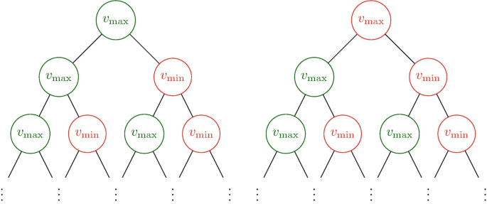

  

  The first branches of the binary tree used for sampling the velocity

  Remark 11

  Notice that the control policy RE may have a very large total variation, and thus it might not respect the bounds on TV given in (1). Therefore, the found control policies may not be allowed as a solution of this problem. However, this technique was implemented for comparison with the results and performances obtained by the GDM.

• Gradient descent method First, numerically one-sided variations of the cost are computed using (4.14). Then, the classical gradient descent method [4] is used to find the optimal control strategy and to compute the optimal velocity that fits the given outflow profile.

4.3.4.3 Simulations

The following parameters: $L=1, \; \mathcal {J}=100,\; T=15.0,\; u_{\mathrm {cr}}= 0.5,\; u_{\max }=1, \; v_{\min } = 0.5,$ and $v_{\max }= 1.0$ are chosen. Moreover, the input flux at the boundary of the domain is given by $\mbox{In} = \min {(0.3+0.3\sin {}(2\pi t^n),0.5)}$. Two different target fluxes f ^∗ = 0.3 and $f^* = \left \vert (0.4\sin {}(t\pi - 0.3)) \right \vert$ are used. The initial condition is a constant density u(0, x) = 0.4, and oscillating inflows to represent variations in typical inflow of urban or highway networks at the 24 h time scale are given.

4.3.4.3.1 Test I: Constant Outflow

In Fig. 4.5, the time-varying speed obtained by using the three policies is shown. In each case, we notice that due to the oscillating input signal the control policy is also oscillating. From a practical point of view, a solution where the speed changes at each time step might be unfeasible, but these policies could be seen as periodic change of maximal speed for different time frames during the day when the time horizon is scaled to the day length. In Table 4.1, one can see the different results obtained for the cost functional computed at the final time for the different policies. The instantaneous policy is outperformed by the random exploration policy and by the gradient method. In Fig. 4.6, one can see the distribution of the different values of the cost functional over 1000 simulations. Moreover, in Fig. 4.7, one can see the differences between the actual outflow obtained and the target one for all methods. The CPU time for the different simulations approaches (see Table 4.2) is compared, and as expected, the random exploration policy is the least performing, while the instantaneous policy is the fastest one. In addition, one can look at the TV(v) for each one of the policies obtaining the following results:

Fig. 4.5

Speed obtained by using the instantaneous policy (left), random exploration policy (center), and the gradient descent method (right) for a target flux f ^∗ = 0.3

Fig. 4.6

Histogram of the distribution of the value of the cost functional for the random exploration policy. We run 1000 different simulations

Fig. 4.7

Difference between the real outgoing flux and the target constant flux, computed with the instantaneous policy (left), the gradient method (right) and the random exploration policy (center)

Table 4.1 Value of the cost functional and the average velocity for the different policies

Table 4.2 CPU time for the simulations performed with the different approaches

• IP: TV(v) = 12.6904

• RE: TV(v) = 753.5

• GDM: TV(v) = 70.81333

Notice that the simple case of a fixed speed has TV(v) = 0, making this option the most performing from this point of view.

4.3.4.3.2 Test II: Sinusoidal Outflow

In Fig. 4.8, it is shown the optimal velocity obtained by using the instantaneous policy, the random exploration, and the gradient descent method with a sinusoidal outflow. One can see that the different policies give different profiles of optimal speed. In each case, we can see that an a posteriori treatment of the speeds before implementation in real traffic might be needed. Figure 4.9 shows the histogram of the cost functional obtained for the random exploration policy, and in Fig. 4.10, the real outgoing flux with the target one is compared. In Table 4.3, different results obtained for the cost functional computed at final time for the different policies are shown. Also, in this case, the instantaneous policy is outperformed by the other two. The CPU times give results similar to the previous test.

Fig. 4.8

Speed obtained by using the instantaneous policy (left), the gradient descent method (right), and the random exploration policy (center) for a sinusoidal target flux

Fig. 4.9

Histogram of the distribution of the value of the cost functional for the random exploration policy. We run 1000 different simulations

Fig. 4.10

Difference between the real outgoing flux and the target sinusoidal flux, computed with the instantaneous policy (top left), the gradient method (top right), and the random exploration policy (bottom)

Table 4.3 Value of the cost functional for the different policies

4.4 Discrete-Optimization Methods for First Order Models

In this section, we consider variable speed limit (VSL) control problem coupled to ramp metering for first order equations, i.e., the LWR model. In particular, merging these two problems means that on one side we have a conservation law with time-dependent discontinuous coefficients due to the fact that the maximal velocity for the VSL problem must be evaluated at discrete points in time. On the other hand, the on-ramp metering problem corresponds to controlling the boundary conditions at junctions [143, 144]. The resulting optimal control problem is then a combination of two controls directly influencing each other.

We apply continuous optimization techniques, where the first order optimality system is derived and solved by a descent type method [188, 257]. More precisely, we work on the approximate dynamics, thus resulting in the so-called discretize-then-optimize approach leading to a finite-dimensional optimality system [160].

4.4.1 Traffic Flow Network Modeling

As detailed in Appendix B, a traffic flow network can be modeled as a directed graph $\mathcal {G} = (\mathcal {I},\mathcal {J})$, where the edges $\mathcal {I}=\{I_\ell \}_\ell$ correspond to roads and the vertices $\mathcal {J}=\{J_j\}_j$ to junctions or intersections. Each edge $I_\ell \in \mathcal {I}$ is represented by an interval [0, L _ℓ] and u _ℓ(x, t) denotes the density of cars on road I _ℓ.

Given initial conditions u _ℓ(x, 0), the dynamics on the network is described by the LWR equation

$$\displaystyle \begin{aligned} \partial_t u_\ell(t,x) + \partial_x f_\ell(u_\ell(t,x),t) = 0 \qquad \forall \ell,\ x\in\, ]0,L_\ell[,\ t\in[0,T]\end{aligned} $$

(4.20)

with Greenshields flux

$$\displaystyle \begin{aligned} f_\ell(t, u) = u\, v_{\max}^\ell (t) \left( 1 - \frac{u}{u_{\max}^\ell} \right) \,, \end{aligned}$$

where $v_{\max }^\ell (t)$ is the (piecewise constant) maximal speed limit and $u_{\max }^\ell$ is the maximal car density corresponding to the jammed situation, see, for instance, Fig. 4.11. The maximal flux $f^{\max }_\ell (t)$ is attained at $u=u_{\mathrm {cr}}^\ell =u_{\max }^\ell /2$, see Fig. 4.11.

Fig. 4.11

Velocity and flow rate for different values of $v_{ \max }^\ell (t)$

4.4.1.1 Coupling Conditions at Junctions

The dynamics at junction nodes $J_j\in \mathcal {J}$ must guarantee mass conservation and is defined using the demand and supply functions corresponding to f _ℓ(t, u):

In the rest of this section, only the cases of one-to-one, merging, and diverging junctions are considered, i.e., Fig. 4.12.

Fig. 4.12

Different types of junctions. (a) One-to-one. (b) Diverging. (c) Merging

The coupling conditions are computed as follows:

• One-to-one junction: the fluxes at the junction are obtained by

  

  (4.21)

• Diverging junction: the distribution of cars on outgoing roads is described by the parameters α _2,1 ≥ 0 and α _3,1 ≥ 0 such that α _2,1 + α _3,1 = 1, and the fluxes at the junction are given by the following (non-FIFO) conditions [176, 205]:

  

  (4.22a)
  

  (4.22b)
  $$\displaystyle \begin{aligned}\begin{array}{r*{20}l} \hat\gamma_{1} & = \hat\gamma_{2} + \hat\gamma_{3} {}\,. \end{array}\end{aligned} $$

  (4.22c)

• Merging junction: we introduce a priority parameter P ∈ (0, 1), and the fluxes are given by

  

  (4.23a)
  

  (4.23b)
  $$\displaystyle \begin{aligned}\begin{array}{r*{20}l} \hat\gamma_{3} & = \hat\gamma_{1} + \hat\gamma_{2} \,.{} \end{array}\end{aligned} $$

  (4.23c)

4.4.1.2 Boundary Conditions

If an arc I _ℓ that is connected to the network only downstream while the desired inflow rate upstream is , the actual inflow to the road I _ℓ is given by

(4.24)

Assuming instead that there is a queue at the upstream node of arc I _ℓ with length l _ℓ(t), then, the inflow to the road is given by

(4.25)

where the demand function depends on the length l _ℓ(t) of the queue at time t,

(4.26)

Above, $\tilde f^{\max }_\ell$ denotes the maximum flux that can enter the road from the queue. The evolution of the queue length l _ℓ(t) is given the ODE

(4.27)

for an initial state l _ℓ(0).

Conversely, on arcs connected only upstream to the network, absorbing boundary conditions are prescribed up to a given maximum flow rate as

(4.28)

thus ensuring that cars exit the network if their flow is lower than the maximum flow rate.

4.4.2 Optimization Problem for VSL and Ramp Metering

In this section, we describe the optimization problem, consisting of minimizing the total travel time [267] and/or maximizing the outflow of the system, controlling traffic flow through a network by adjusting maximal speed limits and on-ramp fluxes:

(4.29)

where we set $\vec {l} = (l_\ell )_\ell$, $\vec {u} = (u_\ell )_\ell$ and $\vec {\gamma }^{\text{out}} = (\gamma _\ell ^{\text{out}})_\ell$. Alternatively, one can choose to minimize a congestion measure as in [247], i.e.,

(4.30)

Above, β _ℓ and denote non-negative weights and v _ℓ,ref a reference velocity.

4.4.2.1 Variable Speed Limits

We assume that the time-dependent maximal velocities $v_{\max }^\ell (t)$ have uniform lower and upper bounds

$$\displaystyle \begin{aligned} v_{\text{low}}^\ell \le v_{\max}^\ell (t) \le v_{\text{high}}^\ell \qquad \forall t\in[0,T] \,. \end{aligned}$$

To get a finite number of speed changes, we introduce control points ν ^k ∈ [0, T], k ∈{0, …, Nu}, and the corresponding control variables $V^k_\ell$ for each road. The maximal speed $v_{\max }^\ell (t)$ is assumed to be piecewise constant on the control grid:

$$\displaystyle \begin{aligned} v_{\max}^\ell(t) = V^{k+1}_\ell \qquad \forall t \in\, ]\nu^k, \nu^{k+1}] \,. \end{aligned} $$

(4.31)

4.4.2.2 Ramp Metering

On-ramp dynamics can be described in the framework of merging junctions, where we set the index ℓ = 2 for the on-ramp, which will be described as a queue (4.26). Here, the aim is to control the main lane access from the on-ramp through a controlled demand function that is defined as

(4.32)

where is given by (4.26). Then, plugging (4.32) in (4.23), we obtain

(4.33a)

(4.33b)

$$\displaystyle \begin{aligned}\begin{array}{r*{20}l} \hat\gamma_{3} & = \hat\gamma_{1} + \hat\gamma_{2} \,.{} \end{array}\end{aligned} $$

(4.33c)

Correspondingly, the evolution of the on-ramp buffer changes to

(4.34)

where is the external boundary inflow at the on-ramp.

For ramp metering, we consider a piecewise constant control function:

$$\displaystyle \begin{aligned} \omega_\ell(t) = \omega^{k+1}_\ell \qquad \forall t \in (\nu^k, \nu^{k+1}] \,. \end{aligned} $$

(4.35)

Finally, the joint speed limit and ramp metering control problem for traffic flow on networks is given by

(4.36)

with $\vec {z} = (z_\ell )_-\ell$ and $\vec {\omega } = (\omega _\ell )_\ell$.

4.4.3 Numerical Simulations

Consider a time mesh t ⁿ = n Δt with $\Delta t = \frac {T}{\mathit {Nt}}$ and divide each road ℓ into Nx _ℓ cells of size $\Delta x_\ell = \frac {L_\ell }{\mathit {Nx}_\ell }$.

The discretized objective functions corresponding to (4.29) and (4.30) are

(4.37)

and

$$\displaystyle \begin{aligned} \min \sum_\ell \beta_\ell \sum_{n=1}^{\mathit{Nt}} \left( l_\ell^n + \max\left\{0, \sum_{j=1}^{\mathit{Nx}_\ell} \left(u_{\ell,j-0.5}^n - \frac{f_\ell(u_{\ell,j-0.5}^n,t^n)}{v_{\ell,\text{ref}}} \right)\, \Delta x_\ell \right\} \right) \, \Delta t \,, \end{aligned} $$

(4.38)

where $v_{\ell ,\text{ref}} = \tfrac 12 v^{\text{high}}_\ell$. The conservation law (4.20) is discretized using a staggered Lax–Friedrichs scheme [216]

(4.39a)

(4.39b)

(4.39c)

where λ =  Δt∕ Δx (skipping the index ℓ) and

$$\displaystyle \begin{aligned} u^n_{\ell, j-0.5} \approx \frac{1}{\Delta x_\ell} \int\limits_{(j-1)\Delta x_\ell}^{j \Delta x_\ell} u_\ell(x,t^n) \, dx \qquad \text{for} \quad j \in \{ 1, \dots, \mathit{Nx}_\ell \}, \ n \in \{0,\dots,\mathit{Nt}\} \,. \end{aligned}$$

4.4.3.1 Optimization Approach

The discrete (finite-dimensional) optimization problem (4.37) is solved with an SQP solver (DONLP2) [258, 259], requiring gradient computation. This is achieved using the adjoint approach, which is recalled below.

Given an objective function J(W, Y ) (here (4.37)), where W denotes the control variables of the discretized model equations (the speed limits $z_\ell ^k$ and the ramp controls $\omega _e^k$) and Y the state variables (densities $u_\ell ^n$, flow rates $f(u_\ell ^n)$, queue lengths $l_\ell ^n$). The discretized model equations are denoted E(W, Y ) = 0. Assuming that the model equations E(W, Y ) = 0 have a unique solution Y = Y (W) for any fixed W, we denote by J(W) = J(W, Y (W)) the reduced problem. Let ξ be the solution of the adjoint equation

$$\displaystyle \begin{aligned} \left(\frac{\partial}{\partial Y} E(W,Y(W))\right)^T \xi = - \left(\frac{\partial}{\partial Y} J(W,Y(W))\right)^T \,, \end{aligned} $$

(4.40)

and the cost gradient can be efficiently computed as

$$\displaystyle \begin{aligned} \frac{\mathit{d}}{\mathit{d} u} J(W,Y(W)) = \frac{\partial}{\partial W} J(W,Y(W)) + \xi^T \frac{\partial}{\partial W} E(W,Y(W)) \,. \end{aligned} $$

(4.41)

4.4.3.2 Numerical Results

This section collects the numerical results corresponding to an example of variable speed limit control and a combined optimization of variable speed limits (VSLs) and ramp metering.

4.4.3.2.1 Variable Speed Limit (VSL) Control

The topology of the considered road network (including distribution rates α and priority parameters P) is shown in Fig. 4.13. Further road properties as well as the initial conditions are given in Table 4.4. Additionally, Fig. 4.14 shows the inflow profiles within the considered time horizon of 1000 seconds.

Fig. 4.13

Road network with two main roads

Fig. 4.14

Inflow profiles for the network in Fig. 4.13

Table 4.4 Properties of the roads in Fig. 4.13

For the described setting, we fix the discretization parameters and an increasing number of control points Nu. We separately minimize the total travel time (with β _ℓ = 10⁻³) and maximize the accumulated outflow at the nodes outA and outB (with ). The results are collected in Table 4.5 and Fig. 4.15, showing that lower travel times/larger outflows are obtained for an increasing number of control points. In particular, compared to the uncontrolled case, where all speed limits are taken at the upper bound, there is an improvement of 1.28%/0.03%.

Fig. 4.15

Optimal control of $v_{ \max }$ for an increasing number of control points

Table 4.5 Optimal travel times/outflows for different numbers of control points

We then compare the results with a fixed discretization but an additional penalty term with weight δ _ℓ ≥ 0 in (4.37):

$$\displaystyle \begin{aligned} \sum_e \delta_e \sum_{n=1}^{\mathit{Nt}} \Delta t \left( \frac{v_e^{\max}(t^n) - v_e^{\max}(t^{n-1})}{v^{\text{high}}_e \Delta t} \right)^2 \, , \end{aligned}$$

which penalizes variations in the control. The resulting optimal controls are provided in Fig. 4.16. Obviously, the additional penalty term leads to smoother optimal solutions.

Fig. 4.16

Optimal control of $v_{ \max }$ with and without penalty term (min. travel time)

4.4.3.2.2 VSL and Coordinated Ramp Metering

In this section, we combine the optimization of variable speed limits and ramp metering. The considered network is shown in Fig. 4.17, and the corresponding parameters are given in Table 4.6. The priority parameter at the on-ramp is P = 0.5 and we take . Figure 4.18 shows the inflow profiles and the maximum outflow. We take Nu = 36 control points and the cost functional (4.38), with the following constraints: a maximum queue size of 50 cars at the entrance of the main road (node “in”) and a maximum queue size of 600 cars at the on-ramp are allowed.

Fig. 4.17

Road network with an on-ramp at the node “on-ramp”

Fig. 4.18

Inflow/max. outflow profiles for the network in Fig. 4.17

Table 4.6 Properties of the roads in Fig. 4.17

In the uncontrolled case (Fig. 4.19), the inflow to the main road from the on-ramp varies from full inflow at the beginning of the simulation (f ⁱⁿ = 0.75) to P ⋅ f ^out = 0.5 due to the congestion at road 2 (outflow at the node “out” is 1.0 and priority parameter P = 0.5). The flow on the on-ramp then increases again up to the maximum flow level () when the maximum possible outflow at the node “out” increases. Finally, the inflow to the main road from the on-ramp decreases to the inflow at this node again (f ⁱⁿ = 0.75) when the queue at the on-ramp is empty.

Fig. 4.19

Inflow on the main road at the on-ramp without optimization

Figures 4.20, 4.21, and 4.22 show the computed optimal controls, the queue lengths at the inflow of the main road and at the on-ramp in the uncontrolled and the optimized cases, and the density at the beginning of road 2, respectively. The speed control is activated during large inflow periods, while the on-ramp control acts on the queue length. Moreover, in the optimal solution, the queue at the entrance of the main road is kept empty, while the queue at the on-ramp displays a large peak when traffic gets congested after about 2 hours due to the reduced density on the main road.

Fig. 4.20

Optimal control of $v_{ \max }(t)$ on road 1b and ω(t) at the on-ramp

Fig. 4.21

Queue at the node “in” and the on-ramp

Fig. 4.22

Density at the beginning of road 2 with and without optimization

4.5 Discrete-Optimization Methods for Second Order Models

In this section, we focus on coupling conditions of road networks at on-ramps, where capacity drops usually occur for high density traffic, see, e.g., [169, 183, 211, 239, 260]. By capacity drop we indicate that the measured outflow of the system is smaller than what it could be in optimal conditions, with differences up to 10% or more [183, 260]. This is due to inefficient driving reaction at the exit of a congested zone (upstream the on-ramp), which reduces the downstream flow compared to free flow conditions [267].

While this cannot be captured by first order models like LWR, the challenge for second order models is to find appropriate conditions which capture the capacity drop phenomenon, while ensuring the conservation of mass and momentum flow. Once these coupling conditions are defined, they can be integrated in a finite-volume type numerical scheme to compute the evolution of traffic conditions on the network.

4.5.1 The Aw–Rascle Model on Networks

Let us introduce the modeling equations given by the Aw–Rascle (AR) model [23] including a relaxation term as originally proposed in [157]. The model consists of a 2 × 2 system of conservation laws for the density and a sort of generalized momentum derived from the (anticipate) acceleration equation. We explain below how it can be extended to the context of networks.

Traffic states are described by the density u _i(x, t) and the mean speed of vehicles v _i(x, t) on each road i at position x and time t.

Given some initial state (u _i(x, 0), v _i(x, 0)) on each road i, the dynamics for x ∈ ]0, L _i[ and t ∈ ]0, T[ are described by [23, 157]

$$\displaystyle \begin{aligned} \left\lbrace \begin{array}{ll} &\partial_t u_i + \partial_x (u_i v_i) = 0,\\ &\partial_t (u_i (v_i + p_i(u_i))) + \partial_x (u_i v_i (v_i + p_i(u_i))) = -u_i \frac{v_i - V_i(u_i)}{\delta}, \end{array} \right. \end{aligned} $$

(4.42)

or, setting y _i = u _i(v _i + p _i(u _i)),

(4.43)

where p _i(u) is a given pressure function satisfying $p_i^{\prime }(u) > 0$ and $u p^{\prime \prime }_i(u) + 2p_i^{\prime }(u)>0$ for all u. The latter condition ensures that, for any constant c > 0, the curve {v + p _i(u) = c} is strictly concave and passes through the origin of the (u, uv)-plane. Moreover, there exists a unique point σ _i(c) maximizing the flux uv along the curve {v + p _i(u) = c}. The relaxation term in the momentum equation expresses the tendency of drivers to adjust their velocity to a desired speed V _i(u), with a relaxation time δ > 0.

Aiming at traffic control applications, in the following, we consider the time-dependent preferential velocity:

$$\displaystyle \begin{aligned} V_i(u,t) = v_{\max}^i (t) \left( 1 - \frac{u}{u_{\max}^i} \right) \end{aligned} $$

(4.44)

and the pressure function (as in [169, 239])

$$\displaystyle \begin{aligned} p_i(u,t) = \frac{v^{\text{ref}}_i (t)}{\gamma_i} \left(\frac{u}{u_{\max}^i}\right)^{\gamma_i} \end{aligned} $$

(4.45)

equipped with maximal density $u_{\max }^i>0$, maximal velocity $v_{\max }^i(t)>0$, reference velocity $v^{\text{ref}}_i (t)>0$, and γ _i > 0. Therefore, also, the source term in (4.43) becomes time-dependent: g _i(u, y) = g _i(u, y, t).

As for first order traffic models, we can define the demand and supply functions for each road i as follows: for a given constant c (corresponding to a fixed value of v + p _i(u)), we have

$$\displaystyle \begin{aligned} \mathit{D}_i(u,c,t) &= \begin{cases} \big( c - p_i(u,t) \big) u & \text{if} \ u \le \sigma_i(c,t),\\ \big( c - p_i(\sigma_i(c,t),t) \big) \, \sigma_i(c,t) & \text{if} \ u \ge \sigma_i(c,t), \end{cases}{} \end{aligned} $$

(4.46)

$$\displaystyle \begin{aligned} \mathit{S}_i(u,c,t) &= \begin{cases} \big( c - p_i(\sigma_i(c,t),t) \big) \, \sigma_i(c,t) & \text{if} \ u \le \sigma_i(c,t),\\ \big( c - p_i(u,t) \big) u & \text{if} \ u \ge \sigma_i(c,t), \end{cases}{} \end{aligned} $$

(4.47)

where

$$\displaystyle \begin{aligned} \sigma_i(c,t) = u_i^{\max} \left(\frac{c\, \gamma_i}{v^{\text{ref}}_i(t) \, (1+\gamma_i)} \right)^{\frac{1}{\gamma_i}} \end{aligned} $$

(4.48)

is the sonic point on the curve {v + p _i(u, t)=c} in the (u, uv)-plane. Figure 4.23 provides an illustration of the considered demand and supply functions.

Fig. 4.23

Demand and supply functions corresponding to u _max = 1, v ^ref = 2, γ = 2, and the given values for c

4.5.1.1 Coupling and Boundary Conditions

We describe here the different type of junctions used later and the corresponding coupling conditions. The considered coupling and boundary conditions can be expressed in terms of mass flow q = uv and “momentum flow” q(v + p _i(ρ)).

4.5.1.1.1 One-to-One Junction

In the case of one-to-one junction, the flow maximization over all admissible states leads to

$$\displaystyle \begin{aligned} q_1 = q_2 = \tilde q = \min\left\{ \mathit{D}_1\big( u_{1}, v_1+p_1(u_{1},t), t \big),\, \mathit{S}_2\big( \tilde u_2, v_1+p_1(u_{1},t), t \big) \right\}, \end{aligned} $$

(4.49)

where $\tilde u_2$ is either obtained by the intersection of the curves

$$\displaystyle \begin{aligned} \{ v_2(U,t) = v_2(U_{2},t) \} \quad \text{and} \quad \{ v_2 + p_2(U,t)= v_1+p_1(u_{1},t)\}\end{aligned} $$

(4.50)

or $\tilde u_2 = 0$.

4.5.1.1.2 On-Ramp at a One-to-One Junction

Let us consider a one-to-one junction with an on-ramp, and the demand D ₂(l, t) at the on-ramp is computed by

$$\displaystyle \begin{aligned} \mathit{D}_2(l,t) = \omega_2(t) \begin{cases} f_2^{\max} & \text{if} \ l > 0,\\ \min\{ f_2^{\text{in}}(t), f_2^{\max} \} & \text{if} \ l = 0, \end{cases}\end{aligned} $$

(4.51)

where l is the length of the queue, ω ₂(t) ∈ [0, 1] is the (time-dependent) metering rate, $f_2^{\text{in}}(t)$ is the “inflow” of cars arriving at the on-ramp, and $f_2^{\max }$ is the maximum flow onto the main road. To get a unique solution, we assign the priority parameter P to road 1 and set

$$\displaystyle \begin{aligned} q_1 &= \min \left\{ \mathit{D}_1\big( u_{1}, W_1(t), t \big),\, \max \left\{ P \mathit{S}_3\big( \tilde u_3, W_1(t), t \big),\, \mathit{S}_3\big( \tilde u_3, W_1(t), t \big) - \mathit{D}_2\big( l_{2}, t \big) \right\} \right\}, {} \end{aligned} $$

(4.52)

$$\displaystyle \begin{aligned} q_2 &= \min \left\{ \mathit{D}_2\big( l_{2}, t \big),\, \max \left\{ (1-P) \mathit{S}_3\big( \tilde u_3, W_1(t), t \big),\, \mathit{S}_3\big( \tilde u_3, W_1(t), t \big) - \mathit{D}_1\big( u_{1}, W_1(t), t \big) \right\} \right\}, {} \end{aligned} $$

(4.53)

$$\displaystyle \begin{aligned} q_3 &= q_1 + q_2 , \end{aligned} $$

(4.54)

where we have set W ₁(t) = v ₁ + p ₁(u ₁, t) and $\tilde u_3$ is either obtained by the intersection of the curves

$$\displaystyle \begin{aligned} \{ v_3(U,t) = v_3(U_{3}, t) \} \quad \text{and} \quad \{ w_3(U,t) = v_1+p_1(u_1,t) \} \end{aligned} $$

(4.55)

or $\tilde u_3 = 0$. The evolution of the queue length at the on-ramp is governed by

$$\displaystyle \begin{aligned} \frac{d\, l_2(t)}{\Delta t} = f^{\text{in}}_2(t) - q_2, \end{aligned} $$

(4.56)

where we may assume l ₂(0) = 0.

4.5.1.1.3 On-Ramp at Origin

To better keep track of vehicles entering the network, we consider an on-ramp at vertexes with only one outgoing road:

$$\displaystyle \begin{aligned} \mathit{D}_1(l,t) = \omega_1(t) \begin{cases} f_1^{\max} & \text{if} \ l > 0,\\ \min\{ f_1^{\text{in}}(t), f_1^{\max} \} & \text{if} \ l = 0 \end{cases} \end{aligned} $$

(4.57)

for the demand at the on-ramp, where l is the length of the queue, ω ₁(t) ∈ [0, 1] is the (time-dependent) metering rate, $f_1^{\text{in}}(t)$ is the inflow of cars arriving at the on-ramp, and $f_1^{\max }$ is the maximum flow onto the road.

Since in this case there is no value for c to evaluate the supply function of the road as in (4.49), we consider an auxiliary left state U ₁ mimicking the desired inflow of the on-ramp. We assume that the velocity of the auxiliary state equals the desired velocity of the road, i.e.,

$$\displaystyle \begin{aligned} U_{1} = \big( u, u \tilde W_2(u,t) \big) \qquad \text{such that} \qquad u V_2(u,t) = \mathit{D}_1(l,t), \end{aligned} $$

(4.58)

where $\tilde W (u,t)= V_2(u,t) +p_2(u,t)$, which is solved by

$$\displaystyle \begin{aligned} u_{\pm} = \frac{u_{\max}^2}{2} \pm \sqrt{\frac{(u_{\max}^2)^2}{4} - \frac{u_{\max}^2 \mathit{D}_1(l,t)}{v_{\max}^2(t)}}. \end{aligned} $$

(4.59)

The choice of u ₋ fulfills $\mathit {D}_2(u_-, \tilde w, t) = \mathit {D}_1(l,t)$.

Finally, we get

$$\displaystyle \begin{aligned} q_1 = q_2 = \tilde q = \min\left\{ \mathit{D}_1(l_1,t),\, \mathit{S}_2\big( \tilde u_2, \tilde W_2(u_-,t), t \big) \right\} \end{aligned} $$

(4.60)

with $\tilde W_2(u_-,t) = V_2(u_-,t) + p_2(u_-,t)$, and $\tilde u_2$ is either obtained by the intersection of the curves

$$\displaystyle \begin{aligned} \{ v_2(U, t) = v_2(U_{2}, t) \} \quad \text{and} \quad \{ w_2(U,t) = \tilde W_2 (u_-,t) \} \end{aligned} $$

(4.61)

or $\tilde u_2 = 0$.

The evolution of the queue at the on-ramp is given by

$$\displaystyle \begin{aligned} \frac{d\, l_1(t)}{\Delta t} = f^{\text{in}}_1(t) - q_1. \end{aligned} $$

(4.62)

4.5.1.1.4 Outflow Conditions

At nodes with only one ongoing road, we consider absorbing boundary conditions up to a given maximum flow rate $f^{\text{out}}_1(t)$:

$$\displaystyle \begin{aligned} q_1 = \min\left\{ \mathit{D}_1\big( u_{1}, v_{1} +p_1 (u_1,t), t \big),\, f^{\text{out}}_1(t) \right\}. \end{aligned} $$

(4.63)

The momentum flow is given by q ₁(v ₁ + p ₁(u ₁, t)).

4.5.2 Numerical Simulations for Aw–Rascle on Network with Control

For the numerical solution of the described model, we consider a finite number of time points t ⁿ = n Δt, where Δt = T∕Nt. Moreover, each road i is divided into Nx _i uniform cells of size Δx _i = L _i∕Nx _i. We also set $\Delta t\, v_{\max }^i \le \Delta x_i$ in all numerical simulations.

4.5.2.1 Numerical Method

System (4.43) is discretized via a fractional step method composed by a first order Godunov scheme for the flux term and an implicit Euler method for the relaxation term.

On each road i, the initial conditions (for j ∈{1, …, Nx _i}) are given by the cell averages

$$\displaystyle \begin{aligned} U_{i,{j-0.5}}^0 = \frac{1}{\Delta x_i} \int\limits_{(j-1)\Delta x_i}^{j \Delta x_i} U_i(x,0) \, \Delta x\, \qquad \mbox{for } j \in \{1,\dots,\mathit{Nx}_i\}\,. \end{aligned} $$

(4.64)

Then, at each time iteration n ∈{0, …, Nt − 1}, we compute

$$\displaystyle \begin{aligned} \tilde U^{n+1}_{i,{j-0.5}} &= U^n_{i,{j-0.5}} - \frac{\Delta t}{\Delta x_{i}} \big( F_{i,j}^n - F_{i,{j-1}}^n \big), & & \text{(transport)} \end{aligned} $$

(4.65)

$$\displaystyle \begin{aligned} U^{n+1}_{i,{j-0.5}} &= \tilde U^{n+1}_{i,{j-0.5}} + \Delta t \, g(U_{i,{j-0.5}}^{n+1}). & & \text{(relaxation)} \end{aligned} $$

(4.66)

The boundary fluxes $F_{i,0}^n$ and $F_{i,\mathit {Nx}_i}^n$ are given via coupling/boundary conditions, while

$$\displaystyle \begin{aligned} F_{i,j}^n = \begin{pmatrix}q_{i,j}^n\\ (v_{i,{j-0.5}}^n +p_i( u_{i,{j-0.5}}^n ,t^n)) \, q_{i,j}^n\end{pmatrix} \qquad \mbox{for } j \in \{1,\dots,\mathit{Nx}_i\}\,, \end{aligned} $$

(4.67)

with

$$\displaystyle \begin{aligned} q_{i,j}^n = \min\left\{ \mathit{D}_i(u_{i,{j-0.5}}^n, w_{i,{j-0.5}}^n, t^n), \, \mathit{S}_i(\tilde u_{i,j}^n, w_{i,{j-0.5}}^n, t^n) \right\}, \end{aligned} $$

(4.68)

where $\tilde u_{i,j}^n$ is either obtained by the intersection of the curves

$$\displaystyle \begin{aligned} \{ v_i(U,t^n) = v_{i,{j+0.5}}^n \} \quad \text{and} \quad \{ v_i^t + p_i(U,t^n) = w_{i,{j-0.5}}^n\} \end{aligned} $$

(4.69)

or $\tilde u_{i,j}^n = 0$, and $w_{i,{j-0.5}}^n= v_{i,{j-0.5}}^n +p_i( u_{i,{j-0.5}}^n ,t^n)$.

4.5.2.2 Numerical Results

We study two different scenarios:

• 1. The capacity drop for a one-to-one junction with on-ramp

• 2. Speed control and coordinated ramp metering for a simple network

4.5.2.3 Capacity Drop

We first focus the attention on the capacity drop effect, cf. [169]. We will show how, increasing the inflow into the network, the outflow will decrease.

We consider the network depicted in Fig. 4.24 consisting of two roads of 1 km length with an on-ramp in between. On both roads, we set $u_{\max } = 180\,\frac {\text{cars}}{\text{km}}$, $v_{\max } = v^{\text{ref}} = 100\,\frac {\text{km}}{\text{h}}$, γ = 2, δ = 0.005 h, and an initial density of $50 \,\frac {\text{cars}}{\text{km}}$. At the origin “in,” we assume a constant (desired) inflow $f^{\text{in}}_1 = 3500\,\frac {\text{cars}}{\text{h}}$. At the on-ramp, we consider time-dependent inflows, starting from $f^{\text{in}}_2 = 500\,\frac {\text{cars}}{\text{h}}$ up to $2500\,\frac {\text{cars}}{\text{h}}$ and down to $500\,\frac {\text{cars}}{\text{h}}$ again. The priority parameter at the on-ramp is P = 0.5.

Fig. 4.24

One-to-one junction with on-ramp

Table 4.7 and Fig. 4.25 show the simulation results for the AR and the LWR model (with Δx = 100 meters and Δt = 1.8 seconds), i.e., the resulting stationary states. The first two columns report the desired and the actual inflow at the on-ramp. The following three values are the resulting density, velocity, and the value of v + p(u) just upstream the on-ramp (end of the first road). The last two columns show the total outflow at the end of the second road.

Fig. 4.25

Actual outflow depending on the desired inflow at the on-ramp for the AR and the LWR model

Table 4.7 Capacity drop effect

We observe that up to $1000\,\frac {\text{cars}}{\text{h}}$ of inflow at the on-ramp, the total inflow (of $4500\,\frac {\text{cars}}{\text{h}}$) is within the capacity of the second road. For higher values, the resulting total flux cannot be received at some point. Then the value of v + p(u) at the end of the first road impacts the total flux entering the second road. As a consequence, the outflow at the end of the second road for the cases $f^{\text{in}}_2 \in \{1500\,\frac {\text{cars}}{\text{h}}, \, 2000\,\frac {\text{cars}}{\text{h}}, \, 2500\,\frac {\text{cars}}{\text{h}} \}$ is lower than the outflow for the cases $f^{\text{in}}_2 \in \{500\,\frac {\text{cars}}{\text{h}}, \, 1000\,\frac {\text{cars}}{\text{h}} \}$. Due to the choice of the priority parameter P = 0.5, the effect of a decreasing outflow while the desired inflow increases stagnates as soon as the fluxes from the first road and the on-ramp are equal, which is the case for $f^{\text{in}}_2 \in \{2000\,\frac {\text{cars}}{\text{h}}, \, 2500\,\frac {\text{cars}}{\text{h}} \}$.

We point out that, even when the inflow at the on-ramp is lowered again, the original state for the same values of $f^{\text{in}}_1$ and $f^{\text{in}}_2$ is not reached. This is due to the fact that the outflow in the congested situation is below the accumulated desired inflows. Therefore, the queue at the origin keeps increasing even though the capacity of the road could handle the desired inflows in the free flow situation.

Considering the same scenario with the LWR model (Sect. 4.4 for details), we see that the outflow increases with the accumulated desired inflows until it reaches the maximum capacity of $4500\,\frac {\text{cars}}{\text{h}} = \frac {u_{\text{max}}}{2} \cdot \frac {v_{\max }}{2}$ (see again Table 4.7 and Fig. 4.25). According to the chosen priority P = 0.5, the actual inflows at the origin and at the on-ramp are $2250\,\frac {\text{cars}}{\text{h}}$ at this stage. Further increasing the inflow at the on-ramp does not affect the situation on the roads. Moreover, unlike the AR model, decreasing the desired inflow $f^{\text{in}}_2$ below $1000\,\frac {\text{cars}}{\text{h}}$ leads back to the original situation (as soon as the queues have emptied).

4.5.2.4 Coordinated Speed Control and Ramp Metering

In this section, we aim at controlling maximal speed limits and on-ramp inflows to minimize the total travel time. The ramp metering rate ω _i(t) in Eqs. (4.51) and (4.57) is used to control the demand at the on-ramp. As in Sect. 4.4, we assume $v_{\max }^i = v_{\max }^i(t) \in [v^{\text{low}}_i,v^{\text{high}}_i]$ is another (piecewise constant) control variable. Regarding the pressure term, we will consider two variants:

• 1. $v^{\text{ref}}_i(t) = v_{\max }^i(t)$, i.e., the pressure term directly depends on the (controllable) speed limit and therefore p _i(u) = p _i(u, t).

• 2. $v^{\text{ref}}_i(t) = v^{\text{high}}_i$, i.e., the pressure term is independent of the current speed limit.

We consider the road network represented in Fig. 4.26 (adapted from [174]) with the road parameters given in Table 4.8. The exponents in the pressure function are γ _i = γ = 2 for all roads and δ = 0.005 h for the relaxation parameter. The priority parameter at the on-ramp is P = 0.5 and $f^{\max } = 2000\,\frac {\text{cars}}{\text{h}}$. At the origin “in,” we consider $f^{\max } = 4000\,\frac {\text{cars}}{\text{h}}$.

Fig. 4.26

Road network with an on-ramp

Table 4.8 Parameters of the roads in Fig. 4.26

We fix a time horizon of T = 3.0 hours and the boundary conditions depicted in Fig. 4.27. We aim at minimizing the total travel time

$$\displaystyle \begin{aligned} \sum_{i=1}^{4} \int\limits_0^T \int\limits_0^{L_i} u_i(x,t) \, \Delta x \, \Delta t \ + \ \sum_{j=1}^2 \int\limits_0^T l_j(t) \, \Delta t\,, \end{aligned} $$

(4.70)

Fig. 4.27

Inflow profiles for the network in Fig. 4.26

given an upper bound of 100 vehicles in the queue of the on-ramp. To solve this optimization task, we apply a first-discretize-then-optimize approach and adjoint calculus.

Table 4.9 shows the total travel time for the AR and LWR models with and without optimal control. The resulting queues for the AR model with scaling of the pressure function ($\frac {\partial p_i}{\partial v_{\max }^i}\ne 0$) are shown in Fig. 4.28. Without control, there is no queue at the on-ramp, while more than 300 cars accumulate in the queue at the origin. With ramp metering alone, the queue at the origin is reduced to zero, and up to 100 cars accumulate in the queue at the on-ramp. When ramp metering and speed control are both implemented, the upper bound of 100 cars is never reached. In the case of speed control alone, we have no queue at the on-ramp, while some cars accumulate at the origin.

Fig. 4.28

Queue at the origin “in” and the on-ramp with and without optimal control

Table 4.9 Optimization results for the network in Fig. 4.26

For the LWR model, both queues stay empty during the whole time horizon even without controls, so the optimization produces the same result. This is due to the inability of the LWR model to capture the capacity drop effect.

Figure 4.29 shows the applied optimal controls.

Fig. 4.29

Optimal control of $v_{ \max }^i(t)$ on road 2 (left) and road 3 (center) and ω(t) at the on-ramp (right)

4.6 Bibliographical Notes

The problem of distributed control for partial differential equations with application to traffic has been addressed in several papers in the literature.

An overview of the variable speed limit approaches can be found in [191]. The first papers dealing with variable speed limit using a discretized system of hyperbolic partial differential equations date back to the end of the nineties [3, 214]. In particular, the work [214] used the speed as control to stabilize the nonlinear hyperbolic PDE even with disturbances in the initial data. In the engineering literature, several papers deal with variable speed limit by controlling a discretized hyperbolic PDE [32, 63, 173, 227, 238]. The control is the speed limit that is used to detect and dissipate shock waves generated by macroscopic traffic models. In [173], the problem is analyzed following a Model Predictive Control approach, where the optimization is obtained using sequential quadratic programming (SPQ), while in [63, 96] the problem is analyzed by using closed loop/feedback approaches. For an overview of the approaches on the continuous hyperbolic partial differential equation, in addition to the papers used in this chapter [116, 153, 193] recently, the work [186] looked at the 1D scalar partial differential equation

$$\displaystyle \begin{aligned} \partial_t u + \partial_x (v(t,x) u(t,x)) = 0, \end{aligned} $$

(4.71)

with VSL applied continuously in time and space along a freeway.

In the last few years, variable speed limit approaches have been used also in the case of moving actuators. In particular, autonomous vehicles can be used to control traffic by adopting specific speed policies, see for example [31, 167].

References

A. Alessandri, A. Di Febbraro, A. Ferrara, and E. Punta. Nonlinear optimization for freeway control using variable-speed signaling. IEEE Transactions on vehicular technology, 48(6):2042–2052, 1999.
G. Allaire. Numerical analysis and optimization. Oxford university press, 2007.
L. Ambrosio, N. Fusco, and D. Pallara. Functions of bounded variation and free discontinuity problems, volume 254. Clarendon Press Oxford, 2000.
A. Aw and M. Rascle. Resurrection of “second order” models of traffic flow. SIAM J. Appl. Math., 60(3):916–938, 2000.
C. Bardos, A.-Y. LeRoux, and J.-C. Nédélec. First order quasilinear equations with boundary conditions. Communications in partial differential equations, 4(9):1017–1034, 1979.
L. D. Baskar, B. De Schutter, and H. Hellendoorn. Model-based predictive traffic control for intelligent vehicles: Dynamic speed limits and dynamic lane allocation. In Intelligent Vehicles Symposium, 2008 IEEE, pages 174–179. IEEE, 2008.
G. Bastin and J.-M. Coron. Stability and Boundary Stabilisation of 1-D Hyperbolic Systems. Number 88 in Progress in Nonlinear Differential Equations and Their Applications. Springer International, 2016.
S. Bianchini and A. Bressan. Vanishing viscosity solutions of nonlinear hyperbolic systems. Annals of Mathematics, 161(1):223–342, 2005.
S. Bianchini and R. M. Colombo. On the stability of the standard Riemann semigroup. Proceedings of the American Mathematical Society, 130(7):1961–1973, 2002.
A. Bressan. Contractive metrics for nonlinear hyperbolic systems. Indiana Univ. Math. J., 37(2):409–421, 1988.
A. Bressan. A contractive metric for systems of conservation laws with coinciding shock and rarefaction curves. J. Differential Equations, 106(2):332–366, 1993.
A. Bressan. The unique limit of the Glimm scheme. Arch. Rational Mech. Anal., 130(3):205–230, 1995.
A. Bressan. Hyperbolic systems of conservation laws, volume 20 of Oxford Lecture Series in Mathematics and its Applications. Oxford University Press, Oxford, 2000. The one-dimensional Cauchy problem.
A. Bressan and R. M. Colombo. The semigroup generated by 2× 2 conservation laws. Archive for rational mechanics and analysis, 133(1):1–75, 1995.
A. Bressan, G. Crasta, and B. Piccoli. Well-posedness of the Cauchy problem for n × n systems of conservation laws. Mem. Amer. Math. Soc., 146(694):viii+134, 2000.
A. Bressan and B. Piccoli. Introduction to the mathematical theory of control. American Institute of Mathematical Sciences (AIMS), Springfield, MO, 2007.
G. Bretti, R. Natalini, and B. Piccoli. Fast algorithms for a traffic flow model on networks. Discrete and Continuous Dynamical Systems - Series B, 6(3):427–448, 2006.
R. C. Carlson, D. Manolis, I. Papamichail, and M. Papageorgiou. Integrated ramp metering and mainstream traffic flow control on freeways using variable speed limits. Procedia - Social and Behavioral Sciences, 48(0):1578–1588, 2012. Transport Research Arena 2012.
A. Csikos, I. Varga, and K. M. Hangos. Freeway shockwave control using ramp metering and variable speed limits. 21st Mediterranean Conference on Control & Automation, pages 1569–1574, 2013.
M. L. Delle Monache, B. Piccoli, and F. Rossi. Traffic regulation via controlled speed limit. SIAM Journal on Control and Optimization, 55(5):2936–2958, 2017.
L. C. Evans and R. F. Gariepy. Measure Theory and Fine Properties of Functions. CRC, 1991.
M. Garavello and B. Piccoli. Conservation laws on complex networks. Ann. Inst. H. Poincaré Anal. Non Linéaire, 26(5):1925–1951, 2009.
M. Garavello and B. Piccoli. Time-varying Riemann solvers for conservation laws on networks. J. Differential Equations, 247(2):447–464, 2009.
J. Glimm. Solutions in the large for nonlinear hyperbolic systems of equations. Communication on pure and applied mathematics, 18:697–715, 1965.
P. Goatin, S. Göttlich, and O. Kolb. Speed limit and ramp meter control for traffic flow networks. Engineering Optimization, 48(7):1121–1144, 2016.
S. K. Godunov. A difference method for numerical calculation of discontinuous solutions of the equations of hydrodynamics. Mat. Sb. (N.S.), 47 (89):271–306, 1959.
J. M. Greenberg. Extensions and amplifications of a traffic model of Aw and Rascle. SIAM Journal on Applied Mathematics, 62(3):729–745, 2001.
M. Gugat, M. Herty, A. Klar, and Leugering. Optimal control for traffic flow networks. Journal of optimization theory and applications, 126(3):589–616, 2005.
Y. Han, D. Chen, and S. Ahn. Variable speed limit control at fixed freeway bottlenecks using connected vehicles. Transportation Research Part B: Methodological, 98:113–134, 2017.
B. Haut and G. Bastin. A second order model of road junctions in fluid models of traffic networks. Networks and Heterogeneous Media, 2(2):227–253, 2007.
A. Hegyi, B. De Schutter, and H. Hellendoorn. Model predictive control for optimal coordination of ramp metering and variable speed limits. Transportation Research Part C, 13(3):185–209, 2005.
A. Hegyi, B. D. Schutter, and J. Hellendoorn. Optimal coordination of variable speed limits to suppress shock waves. IEEE Transactions on Intelligent Transportation Systems, 6(1):102–112, 2005.
M. Herty and A. Klar. Modeling, simulation, and optimization of traffic flow networks. SIAM J. Sci. Comput., 25(3):1066–1087, 2003.
W.-L. Jin, Q.-J. Gan, and J.-P. Lebacque. A kinematic wave theory of capacity drop. Transportation Research Part B: Methodological, 81, Part 1:316 –329, 2015.
I. Karafyllis and M. Papageorgiou. Feedback control of scalar conservation laws with application to density control in freeways by means of variable speed limits. Automatica, 105:228–236, 2019.
C. T. Kelley. Iterative methods for optimization. Society for InÉhematics, Philadelphia, 1999.
B. Khondaker and L. Kattan. Variable speed limit: an overview. Transportation Letters, 7(5):264–278, 2015.
O. Kolb, S. Göttlich, and P. Goatin. Capacity drop and traffic control for a second order traffic model. Networks & Heterogeneous Media, 12(4):663–681, 2017.
J. Lebacque and M. Khoshyaran. First order macroscopic traffic flow models for networks in the context of dynamic assignment. In M. Patriksson and M. Labbé, editors, Transportation Planning, volume 64 of Applied Optimization, pages 119–140. Springer US, 2002.
L. Leclercq, V. L. Knoop, F. Marczak, and S. P. Hoogendoorn. Capacity drops at merges: New analytical investigations. Transportation Research Part C: Emerging Technologies, 62:171 –181, 2016.
H. Lenz, R. Sollacher, and M. Lang. Nonlinear speed-control for a continuum theory of traffic flow. IFAC Proceedings Volumes, 32(2):8339–8344, 1999.
R. Leveque. Finite volume methods for hyperbolic problems. Cambridge University Press, Cambridge, UK, 2002.
X.-Y. Lu, T. Z. Qiu, P. Varaiya, R. Horowitz, and S. E. Shladover. Combining variable speed limits with ramp metering for freeway traffic control. In Proceedings of the 2010 American control conference, pages 2266–2271. IEEE, 2010.
M. Papageorgiou, E. Kosmatopoulos, and I. Papamichail. Effects of variable speed limits on motorway traffic flow. Transportation Research Record, 2047(1):37–48, 2008.
C. Parzani and C. Buisson. Second-order model and capacity drop at merge. Transportation Research Record: Journal of the Transportation Research Board, 2315:25–34, 2012.
J. Reilly, W. Krichene, M. L. Delle Monache, S. Samaranayake, P. Goatin, and A. M. Bayen. Adjoint-based optimization on a network of discretized scalar conservation law PDEs with applications to coordinated ramp metering. Journal of optimization theory and applications, 167(2):733–760, 2015.
P. Spellucci. Numerische Verfahren der Nichtlinearen Optimierung. Birkhäuser-Verlag, Basel, 1993.
P. Spellucci. A new technique for inconsistent QP problems in the SQP method. Math. Methods Oper. Res., 47(3):355–400, 1998.
P. Spellucci. An SQP method for general nonlinear programs using only equality constrained subproblems. Mathematical Programming, 82(3):413–448, 1998.
A. Srivastava and N. Geroliminis. Empirical observations of capacity drop in freeway merges with ramp control and integration in a first-order model. Transportation Research Part C: Emerging Technologies, 30:161–177, 2013.
M. Treiber and A. Kesting. Traffic flow dynamics. Springer, Heidelberg, 2013. Data, models and simulation, Translated by Treiber and Christian Thiemann.
Author information
Authors and Affiliations
Rights and permissions
Open Access This chapter is licensed under the terms of the Creative Commons Attribution 4.0 International License (http://creativecommons.org/licenses/by/4.0/), which permits use, sharing, adaptation, distribution and reproduction in any medium or format, as long as you give appropriate credit to the original author(s) and the source, provide a link to the Creative Commons license and indicate if changes were made.
The images or other third party material in this chapter are included in the chapter's Creative Commons license, unless indicated otherwise in a credit line to the material. If material is not included in the chapter's Creative Commons license and your intended use is not permitted by statutory regulation or exceeds the permitted use, you will need to obtain permission directly from the copyright holder.
Copyright information
© 2022 The Author(s)
About this chapter
Cite this chapter
Bayen, A., Monache, M.L.D., Garavello, M., Goatin, P., Piccoli, B. (2022). Distributed Control for Conservation Laws. In: Control Problems for Conservation Laws with Traffic Applications. Progress in Nonlinear Differential Equations and Their Applications(), vol 99. Birkhäuser, Cham. https://doi.org/10.1007/978-3-030-93015-8_4
Download citation
DOI: https://doi.org/10.1007/978-3-030-93015-8_4
Published:
Publisher Name: Birkhäuser, Cham
Print ISBN: 978-3-030-93014-1
Online ISBN: 978-3-030-93015-8
eBook Packages: Mathematics and StatisticsMathematics and Statistics (R0)