Decentralized Control of Conservation Laws on Graphs

Abstract

Conservation and/or balance laws on networks in the recent years have been the subject of intense study, since a wide range of different applications in real life can be covered by such a research.

3.1 Introduction

Conservation and/or balance laws on networks in the recent years have been the subject of intense study, since a wide range of different applications in real life can be covered by such a research. Among the possible applications, vehicular traffic is probably the one more studied; see, for example, [139] and the reference therein. Other applications range over data networks, irrigation channels, gas pipelines, supply chains, and blood circulation; see, for example, [26, 62, 77, 106, 108, 156]. Therefore, it is natural to consider control problems for such systems, and in particular to consider control functions acting at the level of junctions or nodes [144, 160].

This chapter presents various examples of conservation laws with controls acting at the nodes. More precisely, all the examples are motivated by vehicular traffic and so the dynamics in each edge of the network is described by the Lighthill–Whitham–Richards model [224, 249] or by its discrete version.

In Sect. 3.2 we consider a network composed by a single junction and we assume that the control function modifies the junction Riemann solver; see [144]. A junction Riemann solver is a function which gives a solution to every Riemann problems at the node. In this part, we show that, if the Riemann solver and the control function satisfy a suitable set of theoretical assumptions, then there exists a solution of the corresponding Cauchy problem. The section is completed by three concrete examples of Riemann solvers satisfying the required properties.

In Sect. 3.3, we consider a special case of the problem addressed in the previous ones: the regulation of signalized intersections. More precisely, a traffic light can be seen as a regulation of traffic distribution coefficients, that is of the Riemann solver parameters. The controls in this case are piecewise constant and we address the approximation by continuous ones, providing also precise estimation errors. The approach is strongly based on Moscowitz functions, or cumulative counts of cars flowing at a given point, which solve a Hamilton-Jacobi-Bellman equation.

In Sect. 3.4, we consider a freeway model with on-ramps and offramps and the controls act at the level of on-ramps mainly through traffic lights; see [248]. In this part, the highway is described by a finite number of consecutive links, and in each link a discretized version of the Lighthill–Whitham–Richards model is considered. Optimal control problems are studied and necessary conditions for optimality are deduced, by computing a generalized gradient of the cost functional.

In Sect. 3.5, we consider a single road with a spatial non-homogeneity located at position x = x _c; see [79]. More precisely the aim is the description of toll gates or road works in a limited portion of the road. This is obtained by imposing a variable flux constraint at position x = x _c. After giving the definition of solution, we state Theorem 25, which ensure existence and well-posedness of the solution for each admissible control. The section also contains some examples, motivated by applications, of optimal control problems.

Finally, in Sect. 3.6 we consider optimizing the travel time on a loaded network. Solving analytically the problem on a complex network is not feasible thus we resort to optimize some cost function at every junction separately for asymptotic solutions to Riemann Problems. The local problems are solved analytically and the network policies tested numerically. Specifically, we solve analytically the problem for simple junction in Sect. 3.6.1 and simulate the result on two urban networks (in the Italian cities Rome and Salerno) in Sect. 3.6.2. Finally, the case of creating safe corridor for emergency vehicles is addressed in Sect. 3.6.3.

3.2 Control Acting at Nodes Through the Riemann Solver

In this section we consider conservation laws on networks with control acting at the nodes. We refer the reader to Appendix B for notations and basic results of the theory of conservation laws on networks.

We deal with control problems on a node, or more generally on a network with a finite number of arcs and nodes, where the control function ω acts at the level of the node. More precisely, we focus the attention on the following control problem

$$\displaystyle \begin{aligned} \left\{ \begin{array}{l} \begin{array}{l@{\qquad }l} \partial_t\, u_\ell + \partial_x\, f(u_\ell) = 0, & \ell \in \left\{ 1, \cdots, n+m \right\}, \\ u_\ell (0, x) = \bar u_\ell (x), & \ell \in \left\{ 1, \cdots, n+m \right\},\, x \in I_\ell, \end{array} \\ \left( u_{n+1}(t, 0), \cdots, u_{n+m}(t,0) \right) = \mathcal{R}\mathcal{S}_{\omega(t)} \left( u_{1}(t, 0), \cdots, u_{n}(t,0) \right), \end{array} \right. \end{aligned} $$

(3.1)

where ω : [0, +∞[→ Ω is the control function, which acts through the Riemann solver $\mathcal {R}\mathcal {S}$.

3.2.1 The Setting of the Problem

Fix a network composed by a finite number of arcs and nodes. Without loss of generality we focus the attention on a single node J with n incoming arcs I ₁, ⋯ , I _n and m outgoing arcs I _n+1, ⋯ , I _n+m; see [142, Theorem 4.3.9] or [139, Section 4.1]. We model each incoming arc I _i (i ∈{1, ⋯ , n}) of the node with the real interval I _i =] −∞, 0]. Similarly we model each outgoing arc I _j (j ∈{n + 1, ⋯ , n + m}) of the node with the real interval I _j = [0, +∞[. On each arc I _ℓ (ℓ ∈{1, ⋯ , n + m}) we consider the partial differential equation

$$\displaystyle \begin{aligned} \partial_t\, u_\ell + \partial_x\, f (u_\ell) = 0, \end{aligned} $$

(3.2)

where u _ℓ = u _ℓ(t, x) ∈ [0, u _max] is the conserved quantity, and f is the flux. For simplicity, we put u _max = 1.

On the flux f we assume the usual hypothesis

($\mathcal {F}$):

$f : [0, 1] \rightarrow \mathbb {R}$ is a Lipschitz continuous and concave function satisfying

• (a) f(0) = f(1) = 0;

• (b) there exists a unique σ ∈ ]0, 1[ such that f is strictly increasing in [0, σ _l[ and strictly decreasing in ]σ, 1].

Remark 6

A flux f satisfying condition ($\mathcal {F}$) is not an invertible function. However, if we restrict f on the intervals [0, σ] and [σ, 1], both restrictions are invertible. It is convenient to define the restrictions

$$\displaystyle \begin{aligned} \begin{array}{rccc} f_L: & [0, \sigma] & \longrightarrow & \mathbb{R} \\ & u & \longmapsto & f(u) \end{array} \qquad \mbox{and} \qquad \begin{array}{rccc} f_R: & [\sigma, 1] & \longrightarrow & \mathbb{R} \\ & u & \longmapsto & f(u). \end{array} \end{aligned} $$

(3.3)

As said before both f _L and f _R are invertible.

The concept of solution to (3.2) is the following.

Definition 5

Fix ℓ ∈{1, ⋯ , n + m}. A function $u_\ell \in {\mathbf {C}}^{0}([0, +\infty [; {\mathbf {L}}^{1}_{loc} (I_\ell ))$ is an entropy admissible solution to (3.2) in the arc I _ℓ if, for every k ∈ [0, 1] and every $\tilde \varphi : [0, +\infty [ \times I_\ell \to \mathbb {R}$ smooth, positive with compact support contained in $]0,+\infty [ \times \left (I_\ell \setminus \{ 0 \} \right )$, it holds:

$$\displaystyle \begin{aligned} \int_0^{+\infty} \int_{I_\ell} \left[ \left\vert u_\ell -k \right\vert\, \partial_t\, \tilde\varphi + \operatorname{\mathrm{sgn}}(u_\ell - k)\, \left(f (u_\ell)- f(k)\right) \partial_x\, \tilde\varphi \right]\, dx\, dt \ge 0. \end{aligned} $$

(3.4)

Let us introduce the concept of admissible control functions.

Definition 6

We say that ω : [0, +∞[→ Ω is an admissible control function at the node J if:

• 1. Ω is a subset of a normed space $\left (\overline {\Omega }, \left \| \cdot \right \|{ }_{\overline {\Omega }} \right )$;

• 2. Ω is the finite union of connected and pairwise disjoint sets;

• 3. ω is a right continuous function with finite total variation;

• 4. there exists a finite number of jumps between the connected components of Ω.

The definition of Riemann solver at a node is the following one.

Definition 7

A Riemann solver $\mathcal {R}\mathcal {S}$ at J is a function

$$\displaystyle \begin{aligned} \begin{array}{rccc} \mathcal{R}\mathcal{S}: & [0,1]^{n+m} & \longrightarrow & [0,1]^{n+m}\\ & (u_{1,0}, \cdots, u_{n+m,0}) & \longmapsto & (\bar u_1, \cdots, \bar u_{n+m}) \end{array} \end{aligned}$$

satisfying the following properties:

• 1. $\sum _{i=1}^n f_i(\bar u_i)=\sum _{j=n+1}^{n+m} f_j(\bar u_j)$;

• 2. for every i ∈{1, ⋯ , n}, the classical Riemann problem

  

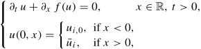
  is solved with waves with negative speed;

• 3. for every j ∈{n + 1, ⋯ , n + m}, the classical Riemann problem

  

  is solved with waves with positive speed;

• 4. the consistency condition

  $$\displaystyle \begin{aligned} \mathcal{R}\mathcal{S}(\mathcal{R}\mathcal{S}(u_{1,0}, \cdots, u_{n+m,0}))= \mathcal{R}\mathcal{S}(u_{1,0}, \cdots, u_{n+m,0}) \end{aligned}$$

  holds.

Fix a family $(\mathcal {R}\mathcal {S}_p)_{p \in \Omega }$ of Riemann solvers at the node J. The concept of solution to (3.1) is given by the following definition.

Definition 8

A collection of functions $u_\ell \in {\mathbf {C}}^{0}([0, +\infty [; {\mathbf {L}}^{1}_{loc}(I_\ell ))$, provides a solution at J to (3.1) if

• 1. for every ℓ ∈{1, ⋯ , n + m}, the function u _ℓ is an entropy admissible solution to (3.2) in the arc I _ℓ;

• 2. for every ℓ ∈{1, ⋯ , n + m} and for a.e. t > 0, the function x↦u _ℓ(t, x) has a version with bounded total variation;

• 3. for a.e. t > 0, it holds

  $$\displaystyle \begin{aligned} \mathcal{R}\mathcal{S}_{\omega(t)} \left(u_1(t, 0), \cdots, u_{n+m}(t,0)\right) = \left(u_1(t, 0), \cdots, u_{n+m}(t,0)\right), \end{aligned} $$

  (3.5)

  where u _ℓ stands for the version with bounded total variation of 2.

3.2.2 The Main Result

Here we state the main result, which deals with the existence of a solution to (3.1). As a preliminary, we need to introduce properties (P1)-(P4) for a family of Riemann solvers $(\mathcal {R}\mathcal {S}_p)_{p \in \Omega }$. These properties ensure some bounds on approximate wave-front tracking solutions, used to prove Theorem 20.

Definition 9

We say that the family of Riemann solvers $(\mathcal {R}\mathcal {S}_p)_{p \in \Omega }$ has the property (P1) if the following condition holds. Given (u _1,0, ⋯ , u _n+m,0) and $(u^{\prime }_{1,0}, \cdots , u^{\prime }_{n+m,0})$ two initial data such that $u_{\ell ,0} = u^{\prime }_{\ell ,0}$ whenever either u _ℓ,0 or $u^{\prime }_{\ell ,0}$ is a bad datum, then

$$\displaystyle \begin{aligned} \mathcal{R}\mathcal{S}_p(u_{1,0}, \cdots, u_{n+m,0}) =\mathcal{R}\mathcal{S}_p(u^{\prime}_{1,0}, \cdots, u^{\prime}_{n+m,0}) \end{aligned} $$

(3.6)

for every p ∈ Ω.

Property (P2) asks for bounds in the increase of the flux variation for waves interacting with J. More precisely the latter should be bounded in terms of the strength of the interacting wave as well as the variation in the incoming fluxes.

Definition 10

We say that the family of Riemann solvers $(\mathcal {R}\mathcal {S}_p)_{p\in \Omega }$ has the property (P2) if there exists a constant C ≥ 1 such that the following condition holds. For every p ∈ Ω, for every equilibrium (u _1,0, ⋯ , u _n+m,0) of $\mathcal {R}\mathcal {S}_p$ and for every wave (u _ℓ,0, u _ℓ) (ℓ ∈{1, ⋯ , n + m}) interacting with J at time $\bar t>0$ and producing waves in the arcs according to the Riemann solver $\mathcal {R}\mathcal {S}_p$, we have

$$\displaystyle \begin{aligned} \begin{array}{c} \mathrm{TV}_f (\bar t+) - \mathrm{TV}_f(\bar t-) \\ \le C \min\left\{\left\vert f(u_{\ell, 0}) - f(u_\ell) \right\vert, \left\vert \Gamma (\bar t+)- \Gamma (\bar t-) \right\vert\right\}. \end{array} \end{aligned} $$

(3.7)

The property (P3) states that a wave interacting with J with a flux decrease on a specific arc should also give rise to a decrease in the incoming fluxes.

Definition 11

We say that the family of Riemann solvers $(\mathcal {R}\mathcal {S}_p)_{p\in \Omega }$ has the property (P3) if, for every p ∈ Ω, for every equilibrium (u _1,0, ⋯ , u _n+m,0) of $\mathcal {R}\mathcal {S}_p$ and for every wave (u _ℓ,0, u _ℓ) (ℓ ∈{1, ⋯ , n + m}) with f(u _ℓ) < f(u _ℓ,0), interacting with J at time $\bar t>0$ and producing waves in the arcs according to the Riemann solver $\mathcal {R}\mathcal {S}_p$, we have

$$\displaystyle \begin{aligned} \Gamma (\bar t+) \le \Gamma (\bar t-). \end{aligned} $$

(3.8)

Finally property (P4) describes the variation of the fluxes due to a variation of the parameter of the Riemann solver.

Definition 12

We say that the family of Riemann solvers $(\mathcal {R}\mathcal {S}_p)_{p\in \Omega }$ has the property (P4) if there exists C > 0 such that, for every p ₁, p ₂ in the same connected component of Ω and for every equilibrium (u _1,0, ⋯ , u _n+m,0) for $\mathcal {R}\mathcal {S}_{p_1}$ we have

$$\displaystyle \begin{aligned} \sum_{\ell=1}^{n+m} \left\vert f(\hat u_\ell) - f(u_{\ell, 0}) \right\vert \le C\left\| p_1 - p_2 \right\|{}_P, \end{aligned} $$

(3.9)

where $(\hat u_1, \cdots , \hat u_{n+m}) =\mathcal {R}\mathcal {S}_{p_2}(u_{1,0}, \cdots , u_{n+m,0})$.

The following result holds.

Theorem 20

Suppose that ω is an admissible control function in the sense of Definition 6 . Assume that, for every ℓ ∈{1, ⋯ , n + m}, $u_\ell \in {\mathbf {L}}^{1} \left (I_\ell ; [0,1]\right )$ with finite total variation. Assume moreover that the family of Riemann solvers $(\mathcal {R}\mathcal {S}_p)_{p\in \Omega }$ satisfies properties (P1)–(P4).

Then there exists a solution (u ₁, ⋯ , u _n+m) to the Cauchy problem (3.1) in the sense of Definition 8.

The proof is based on the wave-front tracking technique; see [144] or [139].

3.2.3 Example of Family of Riemann Solvers

Aim of this part is to present different examples of family of Riemann solvers satisfying properties (P1), (P2), (P3), and (P4).

3.2.3.1 The Riemann Solver $\mathcal {R}\mathcal {S}_1$

This example is based on the Riemann solver introduced for vehicular traffic in [76]. First introduce the set of matrices

$$\displaystyle \begin{aligned} \mathcal{A}:=\left\{ \begin{array}{ll} A=\{a_{ji}\}_{\substack{i=1,\cdots,n\\ j=n+1,\cdots,n+m}}: & \begin{array}{l} 0 < a_{ji} < 1\,\, \forall i,j,\\ \sum_{j=n +1}^{n+m} a_{ji} =1\,\,\forall i \end{array} \end{array} \right\}. \end{aligned} $$

(3.10)

Let {e ₁, ⋯ , e _n} be the canonical basis of $\mathbb {R}^n$. For every i = 1, ⋯ , n, we denote H _i = {e _i}^⊥. If $A\in \mathcal {A}$, then we write, for every j = n + 1, ⋯ , n + m, $a_j=(a_{j1},\cdots ,a_{jn})\in \mathbb {R}^n$ and H _j = {a _j}^⊥. Introduce now the following notation for sets of indices:

• let $\mathcal {H}$ be the set of indices ς = (ς ₁, ⋯ , ς _n) such that $\varsigma _i\in \mathbb {N}$ for every i ∈{1, ⋯ , n} and 1 ≤ ς ₁ < ⋯ < ς _n ≤ n + m;

• let $\mathcal {K}$ be the set of indices k = (k ₁, …, k _ℓ) such that ℓ ∈{1, ⋯ , n − 1}, $k_i\in \mathbb {N}$ for every i ∈{1, ⋯ , ℓ} and 1 ≤ k ₁ < k ₂ < ⋯ < k _ℓ ≤ n + m.

Writing $\mathbf {1}=(1,\cdots ,1)\in \mathbb {R}^n$, for every $\mathbf {k}\in \mathcal {K}$ define

$$\displaystyle \begin{aligned} H_{\mathbf{k}}=\bigcap\limits_{h=1}^\ell H_{k_h} \end{aligned}$$

and the set

$$\displaystyle \begin{aligned} \mathfrak N:=\left\{A\in\mathcal{A}:\mathbf{1}\notin H_{\mathbf{k}}^\bot\, \mbox{ for every } \mathbf{k}\in\mathcal{K} \right\}\,.\end{aligned} $$

(3.11)

Moreover, given 0 < κ ₁ < κ ₂ < 1, define

$$\displaystyle \begin{aligned} \mathfrak N_{\kappa_1}^{\kappa_2}\!=\!\left\{A\in\mathfrak N:\! \kappa_1\le a_{ji}\le\kappa_2,\! \forall i=1,\cdots,n,\forall j=n+1,\cdots,n+m\right\}.\end{aligned} $$

(3.12)

The construction of the Riemann solver $\mathcal {R}\mathcal {S}1$ can be summarized as follows.

• 1. Fix a matrix $A\in \mathfrak N$ and consider the closed, convex, and not empty set

  $$\displaystyle \begin{aligned} \Omega=\left\{ (\gamma_1,\cdots,\gamma_n)\in\prod_{i=1}^n\Omega_i: A\cdot (\gamma_1,\cdots,\gamma_n)^T\in\prod_{j=n+1}^{n+m}\Omega_j \right\}\,.\end{aligned} $$

  (3.13)

• 2. Find the point $(\bar \gamma _1,\cdots ,\bar \gamma _n)\in \Omega$ which maximizes the function

  $$\displaystyle \begin{aligned} E(\gamma_1,\cdots,\gamma_n)=\gamma_1+\cdots+\gamma_n,\end{aligned} $$

  (3.14)

  and define $(\bar \gamma _{n+1},\cdots ,\bar \gamma _{n+m})^T :=A\cdot (\bar \gamma _1,\cdots ,\bar \gamma _n)^T$. Since $A\in \mathfrak N$, the point $(\bar \gamma _1,\cdots ,\bar \gamma _n)$ is uniquely defined.

• 3. For every i ∈{1, ⋯ , n}, set $\bar u_i$ either by u _i,0 if $f(u_{i,0}) = \bar \gamma _i$, or by the solution to $f(u) = \bar \gamma _i$ such that $\bar u_i \ge \sigma _i$. For every j ∈{n + 1, ⋯ , n + m}, set $\bar u_j$ either by u _j,0 if $f(u_{j,0}) = \bar \gamma _j$, or by the solution to $f(u) = \bar \gamma _j$ such that $\bar u_j \le \sigma _j$. Finally, define $\mathcal {R}\mathcal {S}_{1, A}:[0,1]^{n+m} \to [0,1]^{n+m}$ by

  $$\displaystyle \begin{aligned} \mathcal{R}\mathcal{S}_{1,A}(u_{1,0}, \cdots, u_{n+m,0}) =(\bar u_1, \cdots, \bar u_n, \bar u_{n+1}, \cdots, \bar u_{n+m})\,.\end{aligned} $$

  (3.15)

In this way we have defined a family of Riemann solvers $\mathcal {R}\mathcal {S}_{1, A}$ depending on the matrix $A\in \mathfrak N$. For a proof that such a family of Riemann solvers satisfies properties (P1), (P2), (P3), and (P4) see [144] or [139, Chapter 4].

3.2.3.2 The Riemann Solver $\mathcal {R}\mathcal {S}_2$

This example is based on the Riemann solver introduced for telecommunication networks in [108]; see also [139, Chapter 4.2.2]. Consider the set

$$\displaystyle \begin{aligned} \Theta=\left\{\boldsymbol{\theta}=\left(\theta_1,\cdots,\theta_{n+m}\right) \in\mathbb{R}^{n+m}:\, \begin{array}{c} \theta_1>0,\cdots,\theta_{n+m}>0,\\ \sum_{i=1}^n\theta_i=\sum_{j=n+1}^{n+m}\theta_j=1 \end{array} \right\} \end{aligned} $$

(3.16)

of vectors θ, whose components are right of way parameters and so describe the relative importance of the edges of the node. Note that Θ is a convex subset of $\mathbb {R}^{n + m}$; also it is arc-wise connected and so it is a connected subset of $\mathbb {R}^{n + m}$.

The Riemann solver $\mathcal {R}\mathcal {S}_2$ can be constructed with the following steps.

• 1. Fix θ ∈ Θ and define

  $$\displaystyle \begin{aligned} \Gamma_{inc}=\sum_{i=1}^n\sup\Omega_i,\quad \Gamma_{out}=\sum_{j=n+1}^{n+m}\sup\Omega_j, \end{aligned}$$

  then the maximal possible through-flow at the crossing is

  $$\displaystyle \begin{aligned} \Gamma = \min \left\{\Gamma_{inc},\Gamma_{out} \right\}\,. \end{aligned}$$

• 2. Introduce the closed, convex, and not empty sets

  $$\displaystyle \begin{aligned} \begin{array}{rcl} I & = &\displaystyle \left\{ (\gamma_1, \cdots,\gamma_n) \in \prod_{i=1}^n \Omega_i \colon \sum_{i=1}^n \gamma_i = \Gamma \right\} \\ J & = &\displaystyle \left\{ (\gamma_{n+1}, \cdots,\gamma_{n+m}) \in \prod_{j=n+1}^{n+m} \Omega_j \colon \sum_{j=n+1}^{n+m} \gamma_j = \Gamma \right\} \,. \end{array} \end{aligned} $$

• 3. Denote with $(\bar \gamma _1,\cdots ,\bar \gamma _n)$ the orthogonal projection on the convex set I of the point ( Γθ ₁, ⋯ ,  Γθ _n) and with $(\bar \gamma _{n+1},\cdots ,\bar \gamma _{n+m})$ the orthogonal projection on the convex set J of the point ( Γθ _n+1, ⋯ ,  Γθ _n+m).

• 4. For every i ∈{1, ⋯ , n}, define $\bar u_i$ either by u _i,0 if $f(u_{i,0}) = \bar \gamma _i$, or by the solution to $f(u) = \bar \gamma _i$ such that $\bar u_i \ge \sigma _i$. For every j ∈{n + 1, ⋯ , n + m}, define $\bar u_j$ either by u _j,0 if $f(u_{j,0}) = \bar \gamma _j$, or by the solution to $f(u) = \bar \gamma _j$ such that $\bar u_j \le \sigma _j$. Finally, define $\mathcal {R}\mathcal {S}_{2, \boldsymbol {\theta }}: [0,1]^{n+m} \to [0,1]^{n+m}$ by

  $$\displaystyle \begin{aligned} \mathcal{R}\mathcal{S}_{2, \boldsymbol{\theta}} (u_{1,0}, \cdots, u_{n+m,0}) = (\bar u_1, \cdots, \bar u_n, \bar u_{n+1}, \cdots, \bar u_{n+m})\,. \end{aligned} $$

  (3.17)

For a proof that such a family of Riemann solvers satisfies properties (P1), (P2), (P3), and (P4) see [144] or [139, Chapter 4].

3.2.3.3 The Riemann Solver $\mathcal {R}\mathcal {S}_3$

This example is based on the Riemann solver introduced for car traffic in [232] for modeling T-nodes. Consider a node J with n incoming and m = n outgoing arcs and fix a positive coefficient Γ_J, which represents the maximum capacity of the node. The construction of the Riemann solver can be done in the following way.

• 1. Fix θ ∈ Θ, where Θ is defined in (3.16). For every i ∈{1, ⋯ , n}, define

  $$\displaystyle \begin{aligned} \Gamma_i = \min\left\{\gamma_i^{max},\gamma_{i+n}^{max}\right\}, \end{aligned}$$

  then the maximal possible through-flow at J is

  $$\displaystyle \begin{aligned} \Gamma=\sum_{i=1}^n\Gamma_i. \end{aligned}$$

• 2. Introduce the closed, convex, and not empty set

  $$\displaystyle \begin{aligned} I=\left\{(\gamma_1,\cdots,\gamma_n)\in\prod_{i=1}^n[0,\Gamma_i] \colon\sum_{i=1}^n\gamma_i=\min\left\{\Gamma,\Gamma_J\right\}\right\}. \end{aligned}$$

• 3. Denote with $(\bar \gamma _1,\cdots ,\bar \gamma _n)$ the orthogonal projection on the convex set I of the point $\left (\min \{\Gamma ,\Gamma _J\}\theta _1,\cdots , \min \{\Gamma ,\Gamma _J\}\theta _n\right )$ and set $(\bar \gamma _{n+1},\cdots ,\bar \gamma _{2n}) =(\bar \gamma _1,\cdots ,\bar \gamma _n)$.

• 4. For every i ∈{1, ⋯ , n}, define $\bar u_i$ either by u _i,0 if $f(u_{i,0}) = \bar \gamma _i$, or by the solution to $f(u) = \bar \gamma _i$ such that $\bar u_i \ge \sigma _i$. For every j ∈{n + 1, ⋯ , n + m}, define $\bar u_j$ either by u _j,0 if $f(u_{j,0}) = \bar \gamma _j$, or by the solution to $f(u) = \bar \gamma _j$ such that $\bar u_j \le \sigma _j$. Finally, define $\mathcal {R}\mathcal {S}_{3, \boldsymbol \theta }: [0,1]^{n+m} \to [0,1]^{n+m}$ by

  $$\displaystyle \begin{aligned} \mathcal{R}\mathcal{S}_{3, \boldsymbol\theta}(u_{1,0}, \cdots, u_{n+m,0}) = (\bar u_1, \cdots, \bar u_n, \bar u_{n+1}, \cdots, \bar u_{n+m})\,. \end{aligned} $$

  (3.18)

In this way we have defined a family of Riemann solvers $\mathcal {R}\mathcal {S}_{3, \boldsymbol {\theta }}$ depending on the parameter θ. For a proof that such a family of Riemann solvers satisfies properties (P1), (P2), (P3), and (P4) see [144] or [139, Chapter 4].

3.3 Modeling Signalized Intersections

This section is devoted to a specific problem of choosing traffic distribution coefficients: the regulation of signalized intersections. Some technical results will be stated without proofs, referring the reader to [165, 166].

Notice that a traffic signal can be interpreted as a special case of (3.1) with the control signal ω taking values in a discrete set, e.g., {green, red}, and being piecewise constant. The main interest here is to approximate the problem with a continuous one, where the controls represent the traffic distribution coefficients corresponding to a given signal schedule.

The main idea for continuous approximation is as follows. Fix a simple junction with two incoming roads I ₁ and I ₂ and one outgoing I ₃. The main parameter of the problem is the fraction, say η ∈ (0, 1), of the signal cycle for which I ₁ has a green signal, so that 1 − η is the fraction of red signal for I ₁. Then the continuous approximation corresponds to assign a priority to I ₁ so that the resulting fraction of the whole traffic flowing to I ₃, which is coming from I ₁, is equal to η. For a fixed time horizon [0, T], all signal controls will be represented by periodic functions ω _i(⋅) : [0, T] →{0, 1} such that ω _i(t) equals one if the signal is green and equals zero otherwise. We denote by $\Delta _i\in \mathbb {R}_{+}$ the cycle length, i.e., the period of u _i, assume it starts with green and let η _i denote the green fraction.

We parametrize road I _i with the interval $[a_i,\,b_i]\subset \mathbb {R}$, denote by f _i(u) the fundamental diagram (i.e., flux function), by $u^c_i$ the critical density, where the flow is maximal $C_i=f_i(u^c_i)$, and by u ^jam the maximal or jam density. The density on road I _i is denoted by u _i(t, x), for (t, x) ∈ [0, T] × [a _i, b _i]. The demand D _i(t) and supply S _i(t) of the road are given by:

$$\displaystyle \begin{aligned} D_i(t)~=~&\begin{cases} C_i ~~ & \mbox{if}~~u _i(t,\,b_i-) \geq u _i^c \\ f_i\big(u _i(t,\,b_i-)\big)~~ & \mbox{if}~~u _i(t,\,b_i-) < u _i^c \end{cases} \end{aligned} $$

(3.19)

$$\displaystyle \begin{aligned} S_i(t)~=~&\begin{cases} C_i ~~ & \mbox{if}~~u _i(t,\,a_i+) < u _i^c \\ f_i\big(u _i(t,\,a_i+)\big)~~ & \mbox{if}~~u _i(t,\,a_i+) \geq u _i^c; \end{cases} . \end{aligned} $$

(3.20)

The notion of effective supply is of crucial importance to the articulation of signal models.

Definition 13 (Effective Supply)

Given any link I _i, with downstream links {I _j :  j = 1, 2, ⋯ , m _i}, the effective supply for I _i is defined as

(3.21)

where $\alpha _{i,j}(t)\in \mathbb {R}^+$, satisfying $\sum _{j=1}^{m_i}\alpha _{i,j}(t)\equiv 1$, are the car turning percentages, C _i is the flow capacity of the link I _i, and S _j is the supply function for I _j.

The time-varying quantity $\mathcal {E}_i(t)$ expresses the downstream receiving capacity available for I _i if no signal controls is present. The superscripts “Δ” and “0” represent quantities associated with the on-and-off signal model and the continuum signal model, respectively. For given signal control ω _i and effective supply $\mathcal {E}_i(t)$, the on-and-off model is expressed in terms of its downstream boundary condition:

$$\displaystyle \begin{aligned} f^{\Delta}_{out,i}(t)~=~f_i(u _i(t,\, b_i))~=~ \min\Big\{D_i(t),\, \omega_i(t)\mathcal{E}_i(t)\Big\}\qquad \mbox{(On-and-off)}, \end{aligned} $$

(3.22)

where $f^{\Delta }_{out,i}(t)$ is the exit flow, while the continuum signal model is given by:

$$\displaystyle \begin{aligned} f^0_{out,i}(t)~=~f_i(u _i(t,\, b_i))~=~ \min\Big\{D_i(t),\, \eta_i \mathcal{E}_i(t)\Big\}\qquad \mbox{(Continuum)}. \end{aligned} $$

(3.23)

3.3.1 The Hamilton-Jacobi Representation of Signal Models

Denote by N(t, x) the Moskowitz function, i.e., the number of vehicles passed by location x before time t. The function N(t, x) satisfies the following Hamilton-Jacobi equation

$$\displaystyle \begin{aligned} \partial_t N(t,\,x)-f\big(- \partial_x N(t,\,x)\big)~=~0\qquad (t,\,x) \in[0,\,T]\times[a,\,b] \end{aligned} $$

(3.24)

subject to initial condition and boundary conditions. We use a semi-analytic solution representation of the Hamilton-Jacobi equation (3.24), namely the generalized Lax-Hopf formula (see [21, 72]). To isolate a unique solution, we specify the initial condition N _ini(x), the upstream boundary condition N _up(t), and the downstream boundary condition N _down(t) and the weak downstream boundary condition

(3.25)

For the same initial and upstream boundary conditions, the difference in the solution N(t, x) is bounded by the difference in the weak downstream boundary conditions:

$$\displaystyle \begin{aligned} \max_{t\in[0,\,\tau],\,x\in[a,\,b]}\left|N^{\Delta}(t,\,x) - N^0(t,\,x)\right|~\le~\max_{t\in[0,\,\tau]}\left|V^{\Delta}(t)-V^0(t)\right|, \end{aligned} $$

(3.26)

where N ^Δ(t, x) and N ⁰(t, x) represent the Moskowitz function corresponding to the on-and-off and the continuum models, respectively. Our aim is to compare the two signal models studying the convergence of the on-and-off model to the continuum model and determining an error bound on the continuum approximation error. For simplicity let us focus on the simple merge network depicted in Fig. 3.1, with incoming roads I ₁, I ₂ and outgoing ones I ₃. Let ω ₁(t) ∈{0, 1} and ω ₂(t) ∈{0, 1} be the on-and-off signals at the merge junction A, while ω ₃ the one at location B. The presence of the second signal allows to study the effect of the spillback presented in Sect. 3.3.3. We focus on road I ₁ being the analysis for I ₂ similar.

Fig. 3.1

A signalized merge junction

3.3.2 When Spillback Is Absent

We first focus on the case of no spillback at the merge junction A. Our analysis is valid for all fundamental diagrams which satisfy the following condition:

(F) :

the fundamental diagram f(u) of each link is continuous and concave, and vanishes at u = 0 and u = u ^jam.

The lack of spillback at A implies that road I ₃ remains in free flow state, therefore the supply function S ₃(t) of I ₃ is equal to its flow capacity C ₃. The convergence result is given by the following:

Theorem 21

Consider the merge junction of Fig. 3.1 , a signal control ω ₁(⋅) (for link I ₁ ) with cycle length (period of ω ₁ ) indicated by Δ _A , and split parameter (i.e., green-red ratio) η ₁ ∈ (0, 1). Let N _up(t) and N _ini(x) be the upstream boundary condition and initial condition for (3.24) and $N^{\Delta _A}(t,\,x)$ and N ⁰(t, x) be the solutions with additional weak downstream boundary conditions $V^{\Delta _A}(t)$ and V ⁰(t) respectively, given in (3.25). If the entrance of link I ₃ remains in the uncongested phase, then $N^{\Delta _A}(t,\,x) \to N^0(t,\,x)$ uniformly for all (t, x) ∈ [0, T] × [a ₁, b ₁], as Δ _A → 0.

For practical purpose it is important to provide explicit formulas to estimate the error between the solutions produced by continuous and on-and-off signals. We have the following:

Theorem 22 (Error Estimate Without Spillback)

Consider the merge junction of Fig. 3.1 and conditions N _ini(x) and N _up(t) for (3.24) on road I ₁ . Let $N^{\Delta _A}(t,\,x)$ and N ⁰(t, x) be the solutions with additional downstream boundary conditions $V^{\Delta _A}(t)$ and V ⁰(t), given in (3.25). If the entrance of link I ₃ remains in the uncongested phase, then for all (t, x) ∈ [0, T] × [a ₁, b ₁],

$$\displaystyle \begin{aligned} \left|N^{\Delta_A}(t,\,x)-N^0(t,\,x)\right| \le & \eta_1(1-\eta_1)\Delta_A \min\{C_1, C_3\} \\ \le & \frac{1}{4} \Delta_A \min\{C_1,C_3\}. \end{aligned} $$

(3.27)

3.3.3 When Spillback Is Present and Sustained

We turn now to consider the situation when spillback occurs at merge junction A and is sustained (i.e., not absorbed back by the junction for a large number of cycles). Such situation is called sustained spillback and is very common when the demand of roads I ₁ and I ₂ is at high levels and not me by the supply of I ₃.

First we show analytically the lack of convergence for the case of a triangular fundamental diagram:

$$\displaystyle \begin{aligned} f(u )~=~\begin{cases} vu \qquad & \mbox{ if }u \in[0,\,u ^c] \\ -w(u -u ^{jam})\qquad & \mbox{ if }u \in(u ^c,\,u ^{jam}], \end{cases} \end{aligned} $$

(3.28)

where v, respectively w, is the speed of the forward, respectively backward, propagating waves. Notice that V  is also the free flow speed of cars.

Let us first examine the dynamics on road I ₃. Since I ₃ is in congested phase, the characteristic lines with slope − w ₃ (the backward wave speed on I ₃) emit from the right boundary x = b ₃ and reach the left boundary x = a ₃ (see Fig. 3.2). When the light is red, the flow q ₃ exiting I ₃ vanishes, producing a jam density value $u _3^{jam}$, while when the light is green q ₃ is equal to the flow capacity C ₃ generating a density value $u _3^c$ (the critical density on I ₃). As a result, the supply function S ₃(t) at the entrance of I ₃ fluctuates between 0 and C ₃, leading $\mathcal {E}_1(t)$ to fluctuate between 0 and $\min \{C_1,\,C_3\}$.

Fig. 3.2

Wave dynamics on I ₃ in congested phase for a triangular fundamental diagram. The dashed lines represent characteristics traveling backward at speed w ₃

The effective supply $\mathcal {E}_1(t)$ does not have bounded variation as we send the signal cycle of ω ₃(t) to zero. An example is obtained using resonant signals, i.e., ω ₁ and ω ₃ such that S ₃(t) = C ₃ ⋅ ω ₁(t). We get:

$$\displaystyle \begin{aligned} \int_0^t\mathcal{E}_1(\tau) \omega_1(\tau)\,\,\mathrm{d}\tau~=~& \int_0^t \min\{C_1,\,C_3\}\cdot \omega_1^2(\tau)\,\,\mathrm{d}\tau \\ ~=~&\int_0^t \min\{C_1,\,C_3\}\cdot \omega_1(\tau)\,\,\mathrm{d}\tau~=~\int_0^t \mathcal{E}_1(\tau)\,\,\mathrm{d}\tau \end{aligned} $$

which does not converge to $\displaystyle \eta _1\int _0^t \mathcal {E}_1(\tau )\,\,\mathrm {d}\tau$ (regardless of the cycle length Δ_A).

The case of strictly concave fundamental diagram is completely different and we can establish convergence. Assume that f is a piecewise smooth function that satisfies, in addition to (F),

$$\displaystyle \begin{aligned} f''(u )\le -b \qquad \mbox{for some }~ b~>~0 \end{aligned} $$

(3.29)

for all u ∈ [0, u ^jam] such that f is twice differentiable at u. Because of the genuine nonlinearity of the characteristic field, any waves bearing a flux variation, generated by signal control at the exit of the link, is reduced while propagating backward. We are not ready to state our main result, and refer the reader to the papers [165, 166] for detailed proof:

Lemma 2

Consider the merge junction of Fig. 3.1 , assume I ₃ parameterized by [0, L] and a strictly concave fundamental diagram f. Then the supply function S ₃(t) converges to some constant $S_3^*$ uniformly as the cycle length of signal ω ₃(t) tends to zero (Fig. 3.3).

Fig. 3.3

Supply observed at the entrance of I ₃, First row: the triangular case; second row: the strictly concave case. First column: larger signal cycle; second column: smaller signal cycle

The main result for strictly concave case is as follows:

Theorem 23

Consider a network with a fixed-cycle-and-split signal control at each node with a strictly concave fundamental diagram. Then the solution of this network converges to the one corresponding to the continuum signal model, when the traffic signal cycles tend to zero.

For the error estimation we have the following:

Theorem 24 (Error Estimate with Sustained Spillback)

Consider the setting and notations of Theorem 22 , with road I ₃ subject to sustained spillback. If the fundamental diagram of I ₃ is triangular, then

$$\displaystyle \begin{aligned} \left|N^{\Delta_A}(t,x)-N^0(t,x)\right| & \le \eta_1(1-\eta_1) \Delta_A \min\{C_1, C_3\} \\ & \quad +\min\{C_1,C_3\}\,\eta_1 t, \end{aligned} $$

(3.30)

where C ₁ and C ₃ denotes the flow capacity of link I ₁ and I ₃ respectively. If the fundamental diagram of I ₃ is strictly concave, then

$$\displaystyle \begin{aligned} \left|N^{\Delta_A}(t,\,x)-N^0(t,\,x)\right| & \le \min\left\{C_1,\,f\left((f')^{-1}\left({\frac{-L}{L/w+\Delta_B} }\right)\right)\right\} \eta_1 t \\ & \quad + \eta_1(1-\eta_1)\Delta_A \min\{C_1, C_3\} \end{aligned} $$

(3.31)

for all (t, x) ∈ [0, T] × [a ₁, b ₁], where $N^{\Delta _A}(t,\,x)$ and N ⁰(t, x) are the Moskowitz functions with the on-and-off model and the continuum model, respectively. Here Δ _B denotes the cycle length of ω ₃(t).

The next proposition is an immediate consequence of (3.31) and provides useful information on the accuracy of the continuous approximation:

Proposition 5

Assume a strictly concave fundamental diagram f for I ₃ . When spillback occurs, the approximation error |N ^Δ(t, x) − N ⁰(t, x)| decreases with larger length L ₃ of I ₃ , and/or with smaller signal cycle Δ _B . Moreover, the size of the error is determined only by the congested branch of the fundamental diagram.

3.4 Control for a Freeway Model

This section deals with control problems in case of a freeway model with on-ramps and offramps. This kind of problem has been studied by several authors; see, for example, [153, 247, 248] and the references therein.

More precisely, we fix a terminal time T and we consider a finite-horizon control problem on the time interval [0, T].

3.4.1 Freeway Model

We consider a freeway road and we model it with a sequence of N piece of roads, called links and labeled by an index $\ell \in \left \{1, \ldots , N\right \}$. Attached to each link, an onramp and offramp are present.

A discretized version of the Lighthill–Whitham–Richards model [224, 249]

$$\displaystyle \begin{aligned} \partial_t\, u_\ell \left(t,x\right) + \partial_x\, f\left(u_\ell \left(t, x\right)\right) = 0, \end{aligned} $$

(3.32)

along each link I _ℓ is used. We recall that in (3.32) $u_\ell \left (t, x\right )$ represents the density of vehicles on link I _ℓ at time t and position x, and f gives the relationship between the density and the flow of vehicles, a relationship usually called fundamental diagram. Here we assume that the flux function $f: [0, u_{\max }] \to \mathbb {R}$ has the following triangular form [100]:

$$\displaystyle \begin{aligned} f(u) = \min \left\{v u, w (u_{\max} - u), f_{\max}\right\}, \end{aligned} $$

(3.33)

where $v,w,u_{\max }$, and $f_{\max }$ are characteristics of the freeway; see Fig. 3.4.

Fig. 3.4

The flux function f, defined in (3.33)

The discrete model used here is inspired from those developed in [117, 247] and it is suitable for ramp metering applications. The discretization of (3.32) is composed by T time steps, N spatial cells or links, and N on-ramps and offramps. It is developed through a Godunov-based scheme [154, 206].

The state of cell $I_\ell \in \left \{1, \ldots , N\right \}$ at the numerical time $k \in \left \{1,\ldots , T\right ]$ is denoted by $u \left [\ell , k\right ]$, while the number of vehicles on the adjacent onramp is given by $l \left [\ell , k\right ]$. Moreover, we use the following additional functions:

• $\delta \left [\ell , k\right ]$: Maximum flow of vehicles exiting link I _ℓ.

• $\sigma \left [\ell , k\right ]$: Maximum flow of vehicles entering link I _ℓ.

• $d\left [\ell , k\right ]$: Maximum flow of vehicles exiting onramp at link I _ℓ.

• $r^{\max }$: Physical capacity of on-ramps.

• $f^{\text{in}}\left [\ell , k\right ]$: Actual flow entering link I _ℓ.

• $f^{\text{out}}\left [\ell , k\right ]$: Actual flow exiting link I _ℓ.

• $r\left [\ell , k\right ]$: Actual flow exiting onramp I _ℓ.

• $\beta \left [\ell , k\right ]$: Fraction of total flow from link I _ℓ entering link I _ℓ+1 as opposed to offramp of link I _ℓ.

• p: Fraction of mainline flow given priority over onramp flow when merging in congestion.

• $D\left [\ell , k\right ]$: Flow entering onramp of link I _ℓ.

Denoting with Δx and Δt respectively the space and time steps, the discrete system for (3.32) evolves from time k to k + 1 according to the following rules.

$$\displaystyle \begin{aligned} \delta \left[\ell,k\right] & = \min\left\{v u \left[\ell,k\right], f_{\max} \right\} {} \end{aligned} $$

(3.34)

$$\displaystyle \begin{aligned} \sigma\left[\ell,k\right] & = \min\left\{ w\left(u ^{\max} - u \left[\ell,k\right]\right), f_{\max}\right\} {} \end{aligned} $$

(3.35)

$$\displaystyle \begin{aligned} d\left[\ell,k\right] & = \min\left\{ l\left[\ell,k\right] / \Delta t, r^{\max}\right\} {} \end{aligned} $$

(3.36)

$$\displaystyle \begin{aligned} f^{\text{in}}\left[\ell,k\right] & = \min\left\{ \sigma\left[\ell,k\right], d\left[\ell-1,k\right] + \beta\left[\ell,k\right] \delta\left[\ell,k\right] \right\} {} \end{aligned} $$

(3.37)

$$\displaystyle \begin{aligned} f^{\text{out}}\left[\ell,k\right] & = \begin{cases} \delta\left[\ell,k\right] & \mbox{if } \displaystyle \frac{p f^{\text{in}}\left[\ell+1,k\right] }{\beta\left[\ell, k\right] \left(1 + p\right)} \ge \delta\left[\ell, k\right] \\ \displaystyle \frac{f^{\mbox{in}}\left[\ell \!+\! 1,k\right] \!-\! d\left[\ell \!+\! 1,k\right]}{\beta\left[\ell,k\right]} & \mbox{if } \displaystyle \frac{f^{\text{in}}[\ell+1,k]}{1 + p} \ge d\left[\ell+1,k\right] \\ \displaystyle \frac{p f^{\text{in}}\left[\ell+1,k\right]}{\left(1 + p\right) \beta\left[\ell,k\right]} & \mbox{otherwise} \end{cases} \end{aligned} $$

(3.38)

$$\displaystyle \begin{aligned} r\left[\ell, k\right] & = f^{\text{in}}\left[\ell, k\right] - \beta\left[\ell, k\right] f^{\text{out}}\left[\ell, k\right] \end{aligned} $$

(3.39)

$$\displaystyle \begin{aligned} u \left[\ell, k+1\right] & = u \left[\ell, k\right] + \frac{\Delta t}{\Delta x} \left(f^{\text{in}}\left[\ell, k\right] - f^{\text{out}}\left[\ell, k\right]\right) \end{aligned} $$

(3.40)

$$\displaystyle \begin{aligned} l\left[\ell, k+1\right] & = l\left[\ell, k\right] + \Delta t \left(D\left[\ell, k\right] - r\left[\ell, k\right]\right). {} \end{aligned} $$

(3.41)

Equations (3.34)–(3.41) model the merging of onramp and mainline flows, as well as the propagation of congestion waves across the freeway network. The freeway-onramp-offramp junction shown in Fig. 3.5 gives a spatial relation of the state variables.

Fig. 3.5

A freeway-onramp-offramp junction. At time step k, the upstream mainline density $u \left [\ell , k \right ]$ at link I _ℓ and onramp queue $l \left [\ell , k \right ]$ merge and either exit the offramp with a split-ratio of $\left (1 - \beta \right )$ or continue onto the downstream mainline at link I _ℓ+1. The control $\omega \left [\ell , k \right ]$ scales the total demand from onramp $d \left [\ell , k \right ]$ by a factor between 0 and 1

We also introduce a discrete control parameter $\omega \left [\ell , k\right ]\in \left [0,1\right ]$, which represents a scaling factor on the demand of onramp related to I _ℓ at time step k. To this aim, we modify Eq. (3.36) in the following way

$$\displaystyle \begin{aligned} d\left[\ell, k\right] = \omega\left[\ell, k\right]\min \left\{ l\left[\ell, k\right] / \Delta t, r^{\max}\right\}. \end{aligned} $$

(3.42)

3.4.2 Optimal Control Problem

Using the model of Sect. 3.4.1, we develop a method to compute a control $\omega \left [\ell , k\right ]$ for the ramp metering policy, over all the space indices $\ell \in \left \{1, \ldots , N\right \}$ and time $k \in \left \{1, \ldots , T\right \}$, which minimizes, or at least reduces, some specified objective.

More precisely, we consider the minimization of a function, which depends explicitly on the control variables ω and on the state variables u. Note that the state variables u depend on the control variables ω. It is possible to rewrite all the discrete Eqs. (3.34)–(3.35) in the compact way as

$$\displaystyle \begin{aligned} H \left(u, \omega\right) = 0. \end{aligned} $$

(3.43)

Given some cost functional $J\left (u, \omega \right )$, the goal is to find an optimal control ω ^∗ such that, denoting with u ^∗ the corresponding optimal state, we have

$$\displaystyle \begin{aligned} J\left(u^*, \omega^*\right) & = \min_{\omega} \, J \left(u, \omega\right) \end{aligned} $$

(3.44)

$$\displaystyle \begin{aligned} H\left(u^*, \omega^*\right) & = 0 {}. \end{aligned} $$

(3.45)

We compute the gradient of J with respect to the control variables ω, subject to the H constraints (3.45). Referring to the works [148, 160, 270], the generalized gradient of J is

$$\displaystyle \begin{aligned} \nabla_{\omega} J\left(u', \omega'\right) = \frac{\partial J\left(u', \omega'\right)}{\partial u} \frac{d\, u}{d\, \omega} + \frac{\partial J \left(u', \omega'\right)}{\partial \omega}. \end{aligned} $$

(3.46)

By (3.45), the gradient of H with respect to ω is always zero and so

$$\displaystyle \begin{aligned} \nabla_{\omega} H = H_{u} d_{\omega} u + H_{\omega} = 0. \end{aligned} $$

(3.47)

Adding last equation to (3.46) as a Lagrange-like multiplier:

$$\displaystyle \begin{aligned} \nabla_{\omega} J = J_{u} d_{\omega} u + J_{\omega} + \lambda^T \left(H_{u} d_{\omega} u + H_{\omega}\right) = \left(J_{u} + \lambda^T H_{u} \right) d_{\omega} u + \left(J_{\omega} + \lambda^T H_{\omega}\right). \end{aligned}$$

Choosing λ such that $\left (J_{u} + \lambda ^T H_{u} \right ) = 0$, we deduce that

$$\displaystyle \begin{aligned} \nabla_{\omega} J = \left(J_{\omega} + \lambda^T H_{\omega}\right) \ \mbox{such that: } H_{u}^T \lambda = -J_{u}. {} \end{aligned} $$

(3.48)

The system of equations (3.48) is called discrete adjoint system, and we refer to [248] for a comprehensive description of the computation of the adjoint equations for ramp metering. Here we focus on an example focused on a specific application.

3.4.3 Numerical Example

We will now apply the tools of adjoint-based finite-horizon optimal control and multi-objective optimization from the previous section to the case of coordinated ramp metering attacks. Congestion-on-demand describes a class of objectives where an attacker wishes to create congestion patterns of a specific nature. The attacks use a macroscopic freeway model of a 19.4 mile stretch of the I15 South Freeway in San Diego California. The model was split into 125 links with 9 on-ramps and was calibrated using loop-detector measurements available through the PeMS loop-detector system [182]. Figure 3.6a is a Space-time diagram of the I15 freeway. There is no ramp metering control applied to the simulation in Fig. 3.6b, i.e., the ramp meters are always set to green. In order to achieve the congestion-on-demand objective, we need to create a class of objective functions able to represent any jam pattern on the freeway. The method chosen is to maximize the traffic density where we want to put the congestion, while minimizing it everywhere else.

Fig. 3.6

(a) Depicts a space-time diagram of vehicle densities on 19.4 mile stretch of I15 Freeway with no ramp metering. The box objective, and example of congestion-on-demand, is applied in (b)–(d). The user specifies a “desired” traffic jam between postmile 4.5 and 14, for a duration of 20 minutes between 8:20 and 8:40. For this, the α parameter (introduced in Eq. (3.52)) enables the proper design of tradeoffs in the objective

For every cell density value at position i and time k, we assign a coefficient $a_i^k \in \mathbb {R}$. We can then define the corresponding objective function:

$$\displaystyle \begin{aligned} J \left( \mathbf{u}, \boldsymbol{\rho} \right) = \sum_{i = 1}^{N} \sum_{k = 1}^{T} a_i^k \, \rho\left[i,k\right]. \end{aligned} $$

(3.49)

Then, the box objective creates a box of congestion in the space-time diagram, i.e., congestion will be created on a specific segment of the freeway during a user-specified time interval. As there are two competing goals (maximize congestion in the box, minimize congestion elsewhere), the following two objective functions need to be considered:

$$\displaystyle \begin{aligned} f_1 \left( \mathbf{u}, \boldsymbol{\rho} \right) & = - \sum_{(i,k) \in \text{Box}} \rho\left[i,k\right], \end{aligned} $$

(3.50)

$$\displaystyle \begin{aligned} \text{and} \; f_2 \left( \mathbf{u}, \boldsymbol{\rho} \right) & = \sum_{(i,k) \not \in \text{Box}} \rho\left[i,k\right]. \end{aligned} $$

(3.51)

To solve this multi-objective problem, a single parameter $\alpha \in \left [0,1\right ]$ is introduced and the following objective function is minimized:

$$\displaystyle \begin{aligned} J_{\alpha} \left( \mathbf{u}, \boldsymbol{\rho} \right) = \alpha \, f_1 \left( \mathbf{u}, \boldsymbol{\rho} \right) \: + \: \left(1 - \alpha \right) \, f_2 \left( \mathbf{u}, \boldsymbol{\rho} \right), \end{aligned} $$

(3.52)

where α is a trade-off parameter: α = 1 is complete priority on the congestion inside the box, while α = 0 is complete priority on limiting density outside the box.

The results of the box objective are presented in Fig. 3.6b–d. The box of the objective is shown as a black frame with an actual size of 10 miles and 20 minutes. As the trade-off moves from α = 0.3 to 0.9, there is a clear increase in the congestion within the box, at the expense of allowing the congestion to spill outside the desired bounds. In fact, Fig. 3.6d (α = 0.9) activates the bottleneck near the top-left of the box earlier than Fig. 3.6b (α = 0.3) to congest the middle portion of the box, which leads to a propagation of a congestion wave outside the bounds of the bottom-right of the box.

3.5 Optimal Control on Boundary and Flux Constraint

In this part we consider a stretch of road on which the controller can act on the upstream inflow and at a given point of the road by limiting the flow. We deal with the control problem

$$\displaystyle \begin{aligned} \left\{ \begin{array}{l@{\qquad }l} \partial_t\, u + \partial_x\, f(u) = 0 & (t, x) \in \mathbb{R}^+ \times \mathbb{R}^+ \\ u(0, x) = u_0(x) & x \in \mathbb{R}^+ \\ f(u(t, 0)) = \omega_0(t) & t \in \mathbb{R}^+ \\ f(u(t, x_c)) \le \omega_c(t) & t \in \mathbb{R}^+, \end{array} \right. \end{aligned} $$

(3.53)

where u ₀ denotes the initial condition, ω ₀ is the inflow control at x = 0, and ω _c is a time-dependent control imposing a flux constraint at a given position x _c > 0. The flux f is a function satisfying condition ($\mathcal {F}$). Solutions to (3.53) are to be intended according to the following definition.

Definition 14

A function $u \in {\mathbf {C}}^{0} \left ( \mathbb {R}^+; {\mathbf {L}}^{\infty } (\mathbb {R}^+; [0, 1])\right )$ is a weak entropy solution to (3.53) if the following conditions hold.

• 1. For every test function $\varphi \in {\mathbf {C}}_{\mathbf c}^{1} \left ( \mathbb {R}^2; \mathbb {R}^+ \right )$ and for every k ∈ [0, 1]

  $$\displaystyle \begin{aligned} & \int_0^{+\infty} \int_0^{+\infty} \left( \left\vert u - k \right\vert \partial_t\, \varphi + \operatorname{\mathrm{sgn}} (u - k) \left( f(u) - f(k) \right) \partial_x\, \varphi \right) \,\mathrm{d} x \,\mathrm{d} t \\ & + \int_0^{+\infty} \operatorname{\mathrm{sgn}} \left( f_L^{-1}(\omega_0(t)) - k\right) \left(f(u(t, 0+)) - f(k) \right) \varphi(t, 0) \,\mathrm{d} t \\ & + \int_0^{+\infty} \left\vert u_0 - k \right\vert \varphi (0, x) \,\mathrm{d} x + 2 \int_0^{+\infty} \left(1 - \frac{\omega_c(t)}{f(\sigma)} \right) f(k) \varphi(t, x_c)\,\mathrm{d} t \ge 0, \end{aligned} $$

  where f _L is defined in (3.3).

• 2. For a.e. $t \in \mathbb {R}^+$, $f \left (u(t, x_c-)\right ) = f \left ( u(t, x_c+) \right ) \le \omega _c (t)$.

The above entropy condition is inherited from the entropy condition for conservation laws with space-discontinuous fluxes, see, e.g., [187, Definition 1.2]. For alternative equivalent definitions, see [17].

Remark 7

In Definition 14 we denote by u(t, x _c±) the measure theoretic traces of u, which are implicitly defined by

$$\displaystyle \begin{aligned} \lim_{\varepsilon \to 0^+} \frac{1}{\varepsilon} \int_0^{+\infty} \int_{x_c}^{x_c + \varepsilon} \left\vert u(t, x) - u(t, x_c +) \right\vert \varphi (t, x) \,\mathrm{d} x \,\mathrm{d} t & = 0 \\ \lim_{\varepsilon \to 0^+} \frac{1}{\varepsilon} \int_0^{+\infty} \int_{x_c - \varepsilon}^{x_c} \left\vert u(t, x) - u(t, x_c -) \right\vert \varphi (t, x) \,\mathrm{d} x \,\mathrm{d} t & = 0 \end{aligned} $$

for every $\varphi \in {\mathbf {C}}_{\mathbf c}^{1}(\mathbb {R}^2; \mathbb {R})$. Note that both traces at x _c exist and are finite, by [16, Theorem 2.2].

Before stating the well-posedness result for (3.53), we need to introduce the domain

$$\displaystyle \begin{aligned} \mathcal{D} = \left\{ u \in {\mathbf{L}}^{1}\left(\mathbb{R}^+; [0,1] \right): \operatorname{\mathrm{sgn}} (u - \sigma) (f(\sigma) - f(u)) \in \mathbf{BV} (\mathbb{R}^+; \mathbb{R}) \right\}. \end{aligned} $$

(3.54)

Theorem 25

Let ( $\mathcal {F}$ ) holds. Fix $u_0 \in \mathcal {D}$ and $\omega _0, \omega _c \in \mathbf {BV}\left (\mathbb {R}^+; [0, f(\sigma )] \right )$ . Then there exists a unique solution u = u(t, x;u ₀, ω ₀, ω _c) to (3.53) in the sense of Definition 14 and, for every $t \in \mathbb {R}^+$, $u(t, \cdot ;u_0, \omega _0, \omega _c) \in \mathcal {D}$.

Moreover, if $u_0, u^{\prime }_0 \in \mathcal {D}$, $\omega _0, \omega _c, \omega ^{\prime }_0, \omega ^{\prime }_c \in \mathbf {BV}\left (\mathbb {R}^+; [0, f(\sigma )] \right )$ , then, for every t > 0, the following Lipschitz estimate on the corresponding solutions u, u′ holds:

$$\displaystyle \begin{aligned} \left\| u(t) - u'(t) \right\|{}_{{\mathbf{L}}^{1}(\mathbb{R}^+; \mathbb{R})} \le & \left\| u_0 - u^{\prime}_0 \right\|{}_{{\mathbf{L}}^{1}(\mathbb{R}^+; \mathbb{R})} + \left\| \omega_0 - \omega^{\prime}_0 \right\|{}_{{\mathbf{L}}^{1}([0, t]; \mathbb{R})} \\ & + 2 \left\| \omega_c - \omega^{\prime}_c \right\|{}_{{\mathbf{L}}^{1}([0, t]; \mathbb{R})}. \end{aligned} $$

(3.55)

For a proof see [79].

3.5.1 Optimal Control Problems

In this part we deal with optimal control problems related to (3.53). More precisely, in the next paragraphs, we consider some cost functional, motivated by applications.

Queue Length

Assume that at position x _c an obstacle reduces the traffic flow and consequently creates a queue propagating backwards. In this situation, it is reasonable that $\omega _c (t)\equiv \bar \omega _c$, i.e., the flow at x _c due to the presence of the obstacle is constant in time. Introduce, for every $u \in \mathcal {D}$, the congestion set

$$\displaystyle \begin{aligned} \mathcal{C}_u = \left\{ x \in [0, x_c[: \operatorname{\mathrm{sgn}}(u(\xi+) - \sigma) (f(\sigma) - f(u)) = f(\sigma) - \bar \omega_c\, \mbox{ a.e. } \xi \in [x, x_c[\right\}. \end{aligned} $$

(3.56)

The set $\mathcal {D}$ either is empty or is a real interval and represents the locations before the obstacle where the traffic flow is at the maximum level allowed by $\bar \omega _c$. The definition of the queue length functional J _QL is straightforward:

$$\displaystyle \begin{aligned} \begin{array}{rccc} J_{QL}: & \mathcal{D} & \longrightarrow & \mathbb{R}^+ \\ & u & \longmapsto & \left\{ \begin{array}{ll} x_c - \inf \mathcal{C}_u & \mbox{ if } \mathcal{C}_u \ne \emptyset \\ 0 & \mbox{ if } \mathcal{C}_u = \emptyset. \end{array} \right. \end{array} \end{aligned} $$

(3.57)

As pointed out in [79, Proposition 2.5], the cost functional J _QL is upper semicontinuous with respect to the L ¹ topology, but not lower semicontinuous. The consequence is that there exists a control which maximizes the queue length. From the application point of view, it is reasonable to look for a control minimizing J _QL. Unfortunately, the regularity properties of J _QL are not sufficient to prove the existence of a minimizing control.

Stop and Go Waves

The phenomenon of stop & go waves is well documented in engineering literature; see, for example, [189, 266]. The minimization of such waves is an important criterion for management of traffic.

The cost functional J _S&G, for T > 0, is defined by

$$\displaystyle \begin{aligned} \begin{array}{rccc} J_{S\& G}: & \mathcal{D} & \longrightarrow & \mathbb{R}^+ \\ & u & \longmapsto & \displaystyle \int_0^T \int_0^{+\infty} p(x) \,\mathrm{d} \left\vert \partial_x\, v(u) \right\vert \,\mathrm{d} t, \end{array} \end{aligned} $$

(3.58)

where p(x) ∈ [0, 1] is a given weight function, and $\int _0^{+\infty } p(x) \,\mathrm {d} \left \vert \partial _x\, v(u) \right \vert \,\mathrm {d} x$ measures the total variation of the velocity v. By assumption, v is a Lipschitz continuous function; this implies that the function x↦v(u(t, x)) has finite total variation.

Proposition 6

The functional $J_{S \& G}: \mathcal {D} \to \mathbb {R}^+$ , defined in (3.58), is lower semicontinuous with respect to the L ¹ topology. Moreover, given $u_0 \in \mathcal {D}$ and T > 0, there exist $\omega _0^{opt}, \omega _c^{opt} \in \mathbf {BV}(\mathbb {R}^+; [0, f(\sigma )])$ such that

$$\displaystyle \begin{aligned} J_{S \& G}(u^{opt}) = \min_{\omega_0, \omega_c \in \mathbf{BV}(\mathbb{R}^+; [0, f(\sigma)])} J_{S \& G}(u), \end{aligned} $$

(3.59)

where u ^opt denotes the solution to (3.53) with initial condition u ₀ and controls $\omega _0^{opt}, \omega _c^{opt}$ , while u is the solution to (3.53) with initial condition u ₀ and controls ω ₀, ω _c.

For a proof see [80, Lemma 2.1].

Travel Time

The travel time represents a key quantity for drivers to be minimized. Assume that $\bar x > x_c$ is the final destination for drivers starting their trip at x = 0. For simplicity, we also suppose that the initial condition u ₀ ≡ 0. The total quantity of vehicles entering the road in the time interval [0, T] (T > 0) is given by $Q_{in} = \int _0^T \omega _0(t) \,\mathrm {d} t$. Then one can consider the following cost functionals

$$\displaystyle \begin{aligned} J_{TT_1} (\omega_0, \omega_c) & = \frac{1}{Q_{in}} \int_0^{+\infty} t f\left( u(t, \bar x)\right) \,\mathrm{d} t \end{aligned} $$

(3.60)

$$\displaystyle \begin{aligned} J_{TT_2} (\omega_0, \omega_c) & = \frac{1}{Q_{in}} \int_0^{+\infty} t \left[f\left( u(t, \bar x)\right) - f\left( u(t, 0)\right)\right] \,\mathrm{d} t. \end{aligned} $$

(3.61)

The following result holds. For a proof see [79].

Proposition 7

The functionals $J_{TT_1}$ and $J_{TT_2}$ , defined in (3.60) and in (3.61), are Lipschitz continuous with respect to ω ₀ and ω _c . Moreover, given u ₀ ≡ 0, T > 0, and $\bar x > x_c$ , there exist $\omega _0^{opt_1}, \omega _c^{opt_1}, \omega _0^{opt_2}, \omega _c^{opt_2} \in \mathbf {BV}(\mathbb {R}^+; [0, f(\sigma )])$ such that

$$\displaystyle \begin{aligned} J_{TT_1}(u_0^{opt_1}, u_c^{opt_1}) & = \min_{\omega_0, \omega_c \in \mathbf{BV}(\mathbb{R}^+; [0, f(\sigma)])} J_{TT_1}(u) \end{aligned} $$

(3.62)

$$\displaystyle \begin{aligned} J_{TT_2}(u_0^{opt_2}, u_c^{opt_2}) & = \min_{\omega_0, \omega_c \in \mathbf{BV}(\mathbb{R}^+; [0, f(\sigma)])} J_{TT_2}(u). \end{aligned} $$

(3.63)

3.6 Optimization of Travel Time on Networks via Local Distribution Coefficients

In this section we show that optimizing the local traffic distribution coefficients, i.e., solving an optimization problem for the control system (3.1), allows us to find good sub-optimal solutions to the minimization of the travel time over large networks. The results contained in this section are from [64,65,66, 231].

The analytic treatment of an arbitrary network is beyond reach, due to the hybrid nature of the problem, having a continuous evolution and discrete set of parameters. We follow a strategy consisting of the following steps:

Step 1. :

Compute the optimal parameters for the asymptotic behavior of simple networks formed by a single junction.

Step 2. :

For a complex network, use the locally optimal parameters at every junction with a sample-and-hold technique: the current values of data at junctions are used and updated whenever they significantly change.

Step 3. :

Verify the performance of Step 2 comparing, via simulations, with other control strategies.

The first step is a hard task even for simple junctions; thus we focus on two special cases: the 2 × 1 case with two entering and one exiting road; and the 1 × 2 case with one entering and two exiting roads. For the first type of junction, one has only one right of way parameter q and we can solve the problem for different cost functionals. The second type of junctions has no right of way parameters and only one traffic distribution coefficient α. This case is even more complicate and so we address the issue only for a specific cost functional.

3.6.1 Optimization of Simple Networks

Consider a simple network with a single junction with n incoming roads I _i and m outgoing ones I _j. We start performing a heuristic computation of expected traffic load.

Denote by c _φψ, with $\varphi \in \left \{1, \ldots , n\right \}$ and $\psi \in \left \{ n+1, \ldots , n+m\right \}$, the flux from source I _φ to destination I _ψ. Then, the following traffic load are expected on the roads: $u _{\varphi }=\sum \limits _{\psi =n+1}^{n+m}c_{\varphi \psi }$ on road I _φ and $u _{\psi }=\sum \limits _{\varphi =1}^{n}c_{\varphi \psi }$ on road I _ψ. Our strategy is as follows: use u _φ and u _ψ as initial data, solve the corresponding Riemann Problem at the junction, determining the density values $\widehat {u } = \left (\widehat {u}_1, \ldots , \widehat {u}_{n+m} \right )$ at the junction, and use them as expected asymptotic values on the roads to optimize the expected travel times. Consider the following cost functions:

$$\displaystyle \begin{aligned} J_{1} & =\sum_{\varphi =1}^{n}\sum_{\psi =n+1}^{n+m}V_{\varphi \psi }, \\ J_{2} & =\sum_{\varphi =1}^{n}\frac{1}{v_{\varphi }}+\sum_{\psi =n+1}^{n+m} \frac{1}{v_{\psi }}, \\ J_{3} & = \sum_{\varphi =1}^{n}\sum_{\psi =n+1}^{n+m}c_{\varphi \psi }V_{\varphi \psi }, \end{aligned} $$

with V _φψ = v _φ + v _ψ, where $v_{\varphi }=v\left ( \widehat {u }_{\varphi }\right )$ and $v_{\psi }=v\left ( \widehat {u } _{\psi }\right )$ are the velocities on roads I _φ and I _ψ, respectively. Notice that J ₁ gives the average speed over the network, J ₂ the average travel time, while J ₃ the averaged travel time weighted by the flow. We aim at maximizing J ₁ and J ₃, and at minimizing J ₂ with respect to the traffic distribution parameters.

We start considering the case of n = 2 incoming roads and m = 1 outgoing ones, representing a merging. Then, the dynamics is determined by fixing a right of way parameter $q\in \left ] 0,1\right [$; see Appendix B. To state our main results we need to introduce some notation: u _c is the critical density where the flux is maximized, $\gamma ^{max}_i$ indicates the maximal flux on road I _i, q ₁ = q and q ₂ = 1 − q. For incoming roads we set:

$$\displaystyle \begin{aligned} s_{\varphi }=\left\{ \begin{array}{l} \begin{array}{ll} -1 & \text{if}\ u_{\varphi}<u_c \ \text{and}\ \gamma _{1}^{\max}+\gamma_{2}^{\max }\leq \gamma _{3}^{\max }, \\ & \text{or}\ u _{\varphi}<\sigma , \gamma _{3}^{\max}<\gamma_{1}^{\max }+\gamma _{2}^{\max }; \ \text{and}\ q_{\varphi}\widehat{\gamma }_{3}\geq \gamma _{\varphi }^{\max}; \end{array} \\ \begin{array}{ll} +1 & \text{if}\ u _{\varphi}\geq u_c , \\ & \text{or}\ u _{\varphi}<\sigma , \gamma _{3}^{\max}<\gamma_{1}^{\max }+\gamma _{2}^{\max };\ \text{and}\ q_{\varphi}\widehat{\gamma }_{3}<\gamma _{\varphi }^{\max }; \end{array} \end{array} \right. \end{aligned}$$

and for the outgoing one:

$$\displaystyle \begin{aligned} s_{3}=\left\{ \begin{array}{l} \begin{array}{ll} -1 & \text{if}\ u _{3}\leq u_c , \\ & \text{or}\ u _{3}>u_c , \gamma _{1}^{\max}+\gamma_{2}^{\max}<\gamma _{3}^{\max }; \end{array} \\ \begin{array}{ll} +1 & \text{if}\ u _{3}>u_c , \gamma _{1}^{\max}+\gamma_{2}^{\max }\geq \gamma _{3}^{\max }. \end{array} \end{array} \right. \end{aligned}$$

For the simple case of the merge, the functional J ₃ does not depend on the choice of the right of way parameter q, while we can explicitly find the optimal ones for the functionals J ₁ and J ₂, (see [64]):

Theorem 26

Consider a junction J with n = 1 incoming road and m = 2 outgoing roads and define: $k^{-}=\frac {f(\widehat {u}_c)-\gamma _1^{\max }}{\gamma _1^{\max }}$, $k^{+}= \frac {\gamma _2^{\max }}{f(\widehat {u}_c)-\gamma _2^{\max }}$ . The cost functions J ₁ and J ₂ are maximized for the same values of q, given by

• 1. for s ₁ = s ₂ = +1:

  • (a) $q\in \left [ 0,\frac {1}{1+k^{+}}\right ] ,$ if k ⁻≤ 1 ≤ k ⁺ , with k ⁻ k ⁺ > 1, or 1 ≤ k ⁻≤ k ⁺;

  • (b) $q\in \left [ 0,\frac {1}{1+k^{+}}\right [ \cup \left ] \frac {1}{1+k^{-}},1 \right ] ,$ if k ⁻≤ 1 ≤ k ⁺ , with k ⁻ k ⁺ = 1;

  • (c) $q\in \left [ \frac {1}{1+k^{-}},1\right ] ,$ if k ⁻≤ 1 ≤ k ⁺ , with k ⁻ k ⁺ < 1, or k ⁻≤ k ⁺ ≤ 1;

• 2. for s ₁ = s ₂ = −1:

  • (a) $q\in \left [ 0,\frac {1}{1+k^{+}}\right ] ,$ if k ⁻≤ 1 ≤ k ⁺ , with k ⁻ k ⁺ < 1, or k ⁻≤ k ⁺ ≤ 1;

  • (b) $q\in \left [ 0,\frac {1}{1+k^{+}}\right [ \cup \left ] \frac {1}{1+k^{-}},1 \right ]$ , if k ⁻≤ 1 ≤ k ⁺ , with k ⁻ k ⁺ = 1;

  • (c) $q\in \left [ \frac {1}{1+k^{-}},1\right ] ,$ if k ⁻≤ 1 ≤ k ⁺ , with k ⁻ k ⁺ > 1, or 1 ≤ k ⁻≤ k ⁺;

• 3. for s ₁ = −1 = −s ₂: $q\in \left [ \frac {1}{1+k^{-}},1 \right ]$;

• 4. for s ₁ = +1 = −s ₂: $q\in \left [ 0,\frac {1}{1+k^{+}} \right ]$.

Let us now pass to the case of n = 1 incoming road and m = 2 outgoing roads, representing a bifurcation. Let α denote the fraction of traffic flowing from road I ₁ to road I ₂ (while 1 − α is the fraction flowing to road I ₃). The optimization of the functionals J ₁ and J ₂ are similar to the case of merge, while for J ₃ we have the following (see [64]):

Theorem 27

Define:

$$\displaystyle \begin{aligned} \bar\alpha=\frac{\gamma_b^{\max}}{\gamma_b^{\max}+\gamma_c^{\max}}. \end{aligned}$$

If

$$\displaystyle \begin{aligned} \gamma_a^{\max}\leq \min\left\{\frac{\gamma_b^{\max}}{\bar\alpha}, \frac{\gamma_c^{\max}}{1-\bar\alpha}\right\}, \end{aligned} $$

(3.64)

then the maximal value for J ₃ is obtained for all the values of α so that (3.64) holds true with $\bar \alpha$ replaced by α. In the opposite case, J ₃ is maximized only for $\alpha =\bar \alpha$.

3.6.2 Simulations of Two Urban Networks

In this section we use the results stated in Section 3.6.1 to optimize traffic on two urban networks: the first one is a large traffic circle in Rome (Italy), while the second is a small network located in the urban area of the city of Salerno (Italy). More precisely, our first network represents the large traffic circle of the Re di Roma Square. Such network experiences high traffic and congestion every day, also because of the heavy traffic load in the morning rush hours. The square becomes completely stuck with large delays for users. The second network is given by a junction on Via Parmenide, also experiencing high traffic also due to a particularly long red cycle for an incoming road. The result illustrated in this section were developed in [65].

Our aim is to show the effectiveness of the approach also by comparison with other control algorithms, including random ones. Beside the cost functions introduced in Sect. 3.6.1 we will consider stop and go waves so the functional J _S&G introduced in (3.58). We consider the case p(x) ≡ 1 and the flux f(u) = u(1 − u) thus we can rewrite:

$$\displaystyle \begin{aligned} J_{S \& G}=\int_{0}^{T}\int_{\cup I_{i}}\left\vert Dv(u)\right\vert \,\mathrm{d} t \,\mathrm{d} x, \end{aligned}$$

indeed the variation of u is equivalent to that of v(u) = 1 − u. This cost function provides also a measure of safety, since velocity differences are responsible for many accidents.

The Re di Roma Square network consists of junctions with two incoming and one outgoing roads (2 × 1 junctions) and junctions with one incoming and two outgoing roads (1 × 2 junctions). For the latter we consider distribution coefficient given by the road maximal capacities, while we optimize over right of way parameters of the latter. Figure 3.7 (left) illustrate the topology of the network: 2 × 1 junctions (1, 3, 5, 7, 9, 11) are in white, 1 × 2 junctions (2, 4, 6, 8, 10, 12) are in black.

Fig. 3.7

Topology of Re di Roma Square (left) and Via Parmenide crossing in Salerno (right)

The second network consists of a small area of the Salerno urban network, see Fig. 3.7 (right). We are particularly interested in the signalized junction, denoted o, with two incoming roads and one outgoing road. One incoming road, i.e., a − o, is very short and connects Via Picenza to Via Parmenide. The traffic light cycle is of two minutes, with green phase of only 15 seconds for incoming road a − o. Accordingly we set the right of way parameter as follows:

$$\displaystyle \begin{aligned} p=\frac{105}{120}=0.875, \end{aligned}$$

for road b − o, while for road a − o

$$\displaystyle \begin{aligned} q=1-p=1-0.875=0.125. \end{aligned}$$

Simulations are performed over a time interval of T = 30 minutes, with flux function given by f(u) = u(1 − u). At the initial time, roads are empty, thus the density is set to zero. For the first network, we consider the inflow values of 0.3 and 0.75, while for the second network the inflow value is 0.8 for roads entering junction o and 0.3 for the outgoing ones. We compare three cases: (1) right of way parameters optimizing the cost functionals J ₁ and J ₂ called optimal case; fixed right of way parameters, called fixed case) choosing p = 0.2 for first network and p = 0.875 for the second; dynamic random parameters, called dynamic random case, with parameters randomly sampled with uniform distribution at every time step. Figure 3.8 illustrates the time evolution of the cost functional J ₂ for the first network and the different choices of the right of way parameters. Such choices reflect different traffic control policies. The fixed control policy is very poorly performing, while the other two are comparable with the optimal one slightly preferable as shown in the zoomed area Fig. 3.8 (right). Even if the two policies, optimal and random, perform similarly, we can capture the difference in traffic patterns by looking at the functional J _S&G, representing the smoothness of traffic, see Fig. 3.9. The optimal policy significantly outperforms the others. On the other side, the dynamic random choice may generate high oscillations, which in turn compromise safety. For the second network, we consider the cost function J ₁, whose time evolution is depicted in Fig. 3.10. The optimal control policy outperforms the others with an advantage of around 20% in terms of J ₁ values. For the dynamic random choice J ₁ converges numerically to the value corresponding to the fixed parameters p = 0.5 (see [65]). This can be understood as follows. Since the flux is given by f(ρ) = ρ(1 − ρ) we have:

$$\displaystyle \begin{aligned} J_{1}\left( p\right) =\chi -\frac{1}{2}\sqrt{1-4cp}-\frac{1}{2}\sqrt{ 1-4c\left( 1-p\right) }, \end{aligned}$$

where χ and c > 0 are constant, not depending on p. Therefore, $\frac {dJ_{1}\left ( p\right ) }{dp}\geq 0$ if and only if p ∈ [0.5, 1]. In other words, the dynamic random choice approach the worst choice in terms of J ₁.

Fig. 3.8

Time evolution of cost J ₂ for different control policies (left) and zoom (right)

Fig. 3.9

Behavior of the SGW functional in the case of boundary conditions equal to 0.75

Fig. 3.10

Time evolution of cost function J ₁ for the second network (left) and zoom (right)

3.6.3 Emergency Management

We now turn to another optimization problem by focusing on emergency situation. The results in this section were developed in [231].

In heavy loaded network it is important to create safe corridors for emergency vehicles, see Fig. 3.11 for a pictorial presentation of the problem. More precisely, we consider a network made of junctions, each with two incoming and two outgoing roads. Then the dynamics is determined by the traffic distribution coefficients, called α and β (see Appendix B). Naming incoming roads as I ₁ and I ₂ and outgoing ones I ₃ and I ₄, α is the percentage of traffic from road I ₁ going to road I ₃ and similarly β is the percentage of traffic from road I ₂ going to road I ₃.

Fig. 3.11

Cartoon representation of a car accident on a road network and the creation of a safe corridor for emergency vehicles via regulation of the traffic distribution coefficients

The emergency vehicles are assumed to follow a velocity function given by:

$$\displaystyle \begin{aligned} \omega \left( u \right) =1-\delta +\delta v\left( u \right) , {} \end{aligned} $$

(3.65)

with 0 < δ < 1, $v\left ( u \right ) =u (1-u)$ being the velocity of regular traffic. Since $\omega \left ( u _{\max }\right ) =1-\delta >0$, the emergency vehicles travel faster than other vehicles.

The general problem we aim to solve is the following. Given a junction with n incoming roads, say I _φ, φ = 1, …, n, , and m outgoing ones, say I _ψ, ψ = n + 1, …, n + m, and initial data $\left ( u_{\varphi ,0},u _{\psi ,0}\right )$, we aim to maximize the cost:

$$\displaystyle \begin{aligned} W_{\varphi ,\psi }\left( t\right) =\int_{I_{\varphi }}\omega \left( u _{\varphi }\left( t,x\right) \right) \,\mathrm{d} x +\int_{I_{\psi }}\omega \left( u _{\psi }\left( t,x\right) \right) \,\mathrm{d} x. \end{aligned}$$

which gives the traveling time of emergency vehicles on the specific corridor formed by incoming road I _φ and outgoing one I _ψ. As above, we consider the asymptotic state of the Riemann Problem to solve the optimization.

Focusing on 2 × 2 junctions, with I _1,2 incoming roads and I _3,4 outgoing ones, for sufficiently big time T we get:

$$\displaystyle \begin{aligned} W_{\varphi ,\psi }\left( T\right) =\omega \left( \widehat{u }_{\varphi }\right) +\omega \left( \widehat{u }_{\psi }\right) =2-\delta -\frac{ \delta }{2}\left( s_{\varphi }\sqrt{1-4\widehat{\gamma }_{\varphi }}+s_{\psi }\sqrt{1-4\widehat{\gamma }_{\psi }}\right) , {} \end{aligned} $$

(3.66)

where s _φ and s _ψ are defined as:

$$\displaystyle \begin{aligned} s_{\varphi }=\left\{ \begin{array}{ll} +1, & \text{if}\ u _{\varphi ,0}\geq \frac{1}{2},\ \text{or}\ u _{\varphi ,0}< \frac{1}{2}\ \text{and}\ \gamma _{\varphi }^{\max }>\widehat{\gamma }_{\varphi }, \\ -1 & \text{if}\ u _{\varphi ,0}<\frac{1}{2}\ \text{and}\ \gamma _{\varphi }^{\max }= \widehat{\gamma }_{\varphi }, \end{array} \right. \end{aligned}$$

$$\displaystyle \begin{aligned} s_{\psi }=\left\{ \begin{array}{ll} +1, & \text{if}\ u _{\psi ,0}>\frac{1}{2}\ \text{and}\ \gamma _{\psi }^{\max }= \widehat{\gamma }_{\psi }, \\ -1 & \text{if}\ u _{\psi ,0}\leq \frac{1}{2}, \ \text{or}\ u _{\psi ,0}>\frac{1}{2} \ \text{and}\ \gamma _{\psi }^{\max }>\widehat{\gamma }_{\psi }. \end{array} \right. \end{aligned}$$

Fixing, without loss of generality, the safe corridor given by φ = 1 and ψ = 3, we get:

$$\displaystyle \begin{aligned} W_{1,3}\left( T\right) =\omega \left( \widehat{u }_{1}\right) +\omega \left( \widehat{u }_{3}\right) =2-\delta -\frac{\delta }{2}\left( s_{1} \sqrt{1-4\widehat{\gamma }_{1}}+s_{3}\sqrt{1-4\widehat{\gamma }_{3}}\right) . {} \end{aligned} $$

(3.67)

We can find optimal values of the traffic distribution coefficients (see [231]):

Theorem 28

Consider a junction with incoming roads, I ₁ and I ₂ and outgoing ones I ₃ and I ₄ . For T sufficiently big, the cost $W_{1,3}\left (T\right )$ is maximized by the traffic distribution coefficients $\alpha _{opt} =1-\frac {\gamma _{d}^{\max }}{\gamma _{a}^{\max }}$ and any $\beta _{opt}\in \left [0, 1-\frac {\gamma _{d}^{\max }}{\gamma _{a}^{\max }}\right ]$ , with the exception of the following two cases.

If $\gamma _{1}^{\max }\leq \gamma _{4}^{\max }$ then there is no optimal value, but the minimum is approximated by α = ε ₁ and β _opt = ε ₂ , for ε ₁ and ε ₂ small, positive and such that ε ₁ ≠ ε ₂.

Similarly, if $\gamma _{1}^{\max }>\gamma _{3}^{\max }+\gamma _{4}^{\max }$ , then there is no optimal value, but the minimum is approximated by $\alpha =\frac {\gamma _{3}^{\max }}{\gamma _{3}^{\max } +\gamma _{4}^{\max }}-\varepsilon _{1}$ and $\beta =\frac {\gamma _{3}^{\max }}{ \gamma _{3}^{\max }+\gamma _{4}^{\max }}-\varepsilon _{2}$ , with ε _1,2 as for the first case.

To test the effectiveness of the control prescribed by Theorem 28, we compute the cost function evolution and compare with random coefficients, i.e., parameters taken randomly when the simulation starts and then kept constant. More precisely, we consider three scenarios denoted by A, B, and C, with initial data reported in Table 3.1 and boundary conditions coinciding with initial data. The values prescribed by Theorem 28 are as follows: for case A, α _opt = 0.294118 and 0 ≤ β _opt < α _opt (we choose β _opt equal to 0.2); for case B, α _opt = ε ₁, β _opt = ε ₂; for case C, α _opt = 0.708571 + ε ₁, β _opt = 0.708571 + ε ₂. Figures 3.12, 3.13, and 3.14 show the time evolution of the cost function $W_{a,c}\left ( t\right )$ and the values of $W_{a,c}\left ( T\right )$ as function of the two parameters α and β in cases A, B, and C, respectively, with δ = 0.5 and T = 30 minutes. The simulations confirm the optimality of the controls prescribed by Theorem 28. We also notice, especially in Fig. 3.14, that the optimal control may not achieve the best value for transient times, but do so for sufficiently large times.

Fig. 3.12

Case A, evolution of W _a,c(t); left: choice of optimal distribution coefficients (continuous line) and random parameters (dashed lines); right: 3D plots of $W_{a,c} \left ( T \right )$

Fig. 3.13

Case B, evolution of W _a,c(t); left: choice of optimal distribution coefficients (continuous line) and random parameters (dashed lines); right: 3D plots of $W_{a,c} \left ( T \right )$

Fig. 3.14

Case C, evolution of W _a,c(t); left: choice of optimal distribution coefficients (continuous line) and random parameters (dashed lines); right: 3D plots of $W_{a,c} \left ( T \right )$

Table 3.1 Initial conditions for the three simulation cases

3.7 Bibliographical Notes

The possibility of controlling the solutions to conservation laws on networks, by acting on the Riemann solvers through control parameters, has been addressed first in [144] in 2009. A different approach, based on solutions to boundary value problems, has been introduced in [10] in 2018. In the context of road traffic, the setting in [10] fits well with the minimization of travel time or of other meaningful functionals.

The modeling and the (optimal) control of signalized intersections have been widely studied in literature, both from the mathematical [70] and engineering [147, 250, 253, 276] point of view. The approach described in Section 3.3 is based on the papers [165, 166]; see also [139, Chapter 7.1].

In the case of freeways, ramp metering is a widely used strategy for controlling traffic flow without acting directly on the mainline flow or using toll systems. This strategy has been used mostly in connection with microscopic traffic models; see, for example, [37]. The use of feedback controls, in order to obtain a desired flow in the main line, has been studied in various papers [2, 237, 254]. The predictive metering strategy instead uses a model, possibly with uncertainties, for predicting the inflow over a finite time horizon, and consequently it deduces various policies for controlling the flow; see [121, 155, 194]. Section 3.4, based on the paper [247], uses the adjoint calculus for finding solutions to optimal control problem; see also [148, 160, 270, 271].

Conservation laws with flux constraints have been introduced in [78, 140] in 2007. In [78] the problem was presented by a control perspective and a well-posedness result was proved. In [140] the model was proposed for describing the situation of a bottleneck on a road. Various Riemann solvers have been introduced together with existence and uniqueness results. Generalizations on (possibly moving) flux constraints both for scalar equations and for systems were considered in various papers; see [111,112,113,114, 137, 138, 145, 272].

For the optimization of travel time or other significant functional on networks via the choice of distribution of coefficients, see [64, 66, 231].

References

S. Agarwal, P. Kachroo, S. Contreras, and S. Sastry. Feedback-coordinated ramp control of consecutive on-ramps using distributed modeling and Godunov-based satisfiable allocation. IEEE Transactions on Intelligent Transportation Systems, 16(5):2384–2392, 2015. cited By 12.
F. Ancona, A. Cesaroni, G. M. Coclite, and M. Garavello. On the optimization of conservation law models at a junction with inflow and flow distribution controls. SIAM J. Control Optim., 56(5):3370–3403, 2018.
B. Andreianov, C. Donadello, and M. D. Rosini. A second-order model for vehicular traffics with local point constraints on the flow. Math. Models Methods Appl. Sci., 26(4):751–802, 2016.
B. Andreianov, P. Goatin, and N. Seguin. Finite volume schemes for locally constrained conservation laws. Numer. Math., 115(4):609–645, 2010. With supplementary material available online.
J.-P. Aubin, A. Bayen, and P. Saint-Pierre. Dirichlet problems for some Hamilton–Jacobi equations with inequality constraints. SIAM journal on control and optimization, 47(5):2348–2380, 2008.
M. K. Banda, M. Herty, and A. Klar. Gas flow in pipeline networks. Netw. Heterog. Media, 1(1):41–56 (electronic), 2006.
M. Ben-Akiva, D. Cuneo, M. Hasan, M. Jha, and Q. Yang. Evaluation of freeway control using a microscopic simulation laboratory. Transportation Research Part C: Emerging Technologies, 11(1):29–50, 2003. cited By 48.
S. Čanić and E. H. Kim. Mathematical analysis of the quasilinear effects in a hyperbolic model blood flow through compliant axi-symmetric vessels. Math. Methods Appl. Sci., 26(14):1161–1186, 2003.
A. Cascone, C. D’Apice, B. Piccoli, and L. Raritá. Optimization of traffic on road networks. Math. Models Methods Appl. Sci., 17(10):1587–1617, 2007.
A. Cascone, R. Manzo, B. Piccoli, and L. Rarità. Optimization versus randomness for car traffic regulation. Phys. Rev. E, 78:026113, Aug 2008.
A. Cascone, B. Piccoli, and L. Rarita. Circulation of car traffic in congested urban areas. Communications in Mathematical Sciences, 6(3):765–784, 2008.
Y. Chitour and B. Piccoli. Traffic circles and timing of traffic lights for cars flow. Discrete Contin. Dyn. Syst. Ser. B, 5(3):599–630, 2005.
C. Claudel and A. Bayen. Lax–Hopf based incorporation of internal boundary conditions into Hamilton–Jacobi equation. part i: Theory. IEEE Transactions on Automatic Control, 55(5):1142–1157, 2010.
G. M. Coclite, M. Garavello, and B. Piccoli. Traffic flow on a road network. SIAM J. Math. Anal., 36(6):1862–1886 (electronic), 2005.
R. M. Colombo and M. Garavello. A well posed Riemann problem for the p-system at a junction. Netw. Heterog. Media, 1(3):495–511 (electronic), 2006.
R. M. Colombo and P. Goatin. A well posed conservation law with a variable unilateral constraint. J. Differential Equations, 234(2):654–675, 2007.
R. M. Colombo, P. Goatin, and M. D. Rosini. On the modelling and management of traffic. ESAIM Math. Model. Numer. Anal., 45(5):853–872, 2011.
R. M. Colombo and A. Groli. Minimising stop and go waves to optimise traffic flow. Appl. Math. Lett., 17(6):697–701, 2004.
C. Daganzo. The cell transmission model: A dynamic representation of highway traffic consistent with the hydrodynamic theory. Transportation Research Part B, 28:269–287, 1994.
C. D’Apice, S. Göttlich, M. Herty, and B. Piccoli. Modeling, simulation, and optimization of supply chains. Society for Industrial and Applied Mathematics (SIAM), Philadelphia, PA, 2010. A continuous approach.
C. D’Apice, R. Manzo, and B. Piccoli. Packet flow on telecommunication networks. SIAM J. Math. Anal., 38(3):717–740 (electronic), 2006.
M. L. Delle Monache and P. Goatin. A front tracking method for a strongly coupled PDE-ODE system with moving density constraints in traffic flow. Discrete Contin. Dyn. Syst. Ser. S, 7(3):435–447, 2014.
M. L. Delle Monache and P. Goatin. Scalar conservation laws with moving constraints arising in traffic flow modeling: an existence result. J. Differential Equations, 257(11):4015–4029, 2014.
M. L. Delle Monache and P. Goatin. A numerical scheme for moving bottlenecks in traffic flow. Bull. Braz. Math. Soc. (N.S.), 47(2):605–617, 2016. Joint work with C. Chalons.
M. L. Delle Monache and P. Goatin. Stability estimates for scalar conservation laws with moving flux constraints. Netw. Heterog. Media, 12(2):245–258, 2017.
M. L. Delle Monache, J. Reilly, S. Samaranayake, W. Krichene, P. Goatin, and A. M. Bayen. A PDE-ODE model for a junction with ramp buffer. SIAM Journal on Applied Mathematics, 74(1):22–39, 2014.
J. R. Domíngeuz Frejo and E. F. Camacho. Global versus local MPC algorithms in freeway traffic control with ramp metering and variable speed limits. IEEE Transactions on intelligent transportation systems, 13(4):1556–1565, 2012.
M. Garavello and P. Goatin. The Aw-Rascle traffic model with locally constrained flow. J. Math. Anal. Appl., 378(2):634–648, 2011.
M. Garavello, P. Goatin, T. Liard, and B. Piccoli. A multiscale model for traffic regulation via autonomous vehicles. Journal of Differential Equations, 296:6088–6124, 2020.
M. Garavello, K. Han, and B. Piccoli. Models for vehicular traffic on networks, volume 9 of AIMS Series on Applied Mathematics. American Institute of Mathematical Sciences (AIMS), Springfield, MO, 2016.
M. Garavello, R. Natalini, B. Piccoli, and A. Terracina. Conservation laws with discontinuous flux. Netw. Heterog. Media, 2(1):159–179, 2007.
M. Garavello and B. Piccoli. Traffic flow on networks, volume 1 of AIMS Series on Applied Mathematics. American Institute of Mathematical Sciences (AIMS), Springfield, MO, 2006. Conservation laws models.
M. Garavello and B. Piccoli. Time-varying Riemann solvers for conservation laws on networks. J. Differential Equations, 247(2):447–464, 2009.
M. Garavello and S. Villa. The Cauchy problem for the Aw-Rascle-Zhang traffic model with locally constrained flow. J. Hyperbolic Differ. Equ., 14(3):393–414, 2017.
V. Gayah and C. Daganzo. Analytical capacity comparison of one-way and two-way signalized street networks. Transportation Research Record, 2301:76–85, 2012. cited By 33.
M. Giles and S. Ulbrich. Convergence of linearized and adjoint approximations for discontinuous solutions of conservation laws. Part 2: Adjoint approximations and extensions. SIAM Journal on Numerical Analysis, 48(3):905–921, 2010.
P. Goatin, S. Göttlich, and O. Kolb. Speed limit and ramp meter control for traffic flow networks. Engineering Optimization, 48(7):1121–1144, 2016.
S. K. Godunov. A difference method for numerical calculation of discontinuous solutions of the equations of hydrodynamics. Mat. Sb. (N.S.), 47 (89):271–306, 1959.
G. Gomes and R. Horowitz. Optimal freeway ramp metering using the asymmetric cell transmission model. Transportation Research Part C: Emerging Technologies, 14(4):244–262, 2006.
S. Göttlich, M. Herty, and A. Klar. Modelling and optimization of supply chains on complex networks. Commun. Math. Sci., 4(2):315–330, 2006.
M. Gugat, M. Herty, A. Klar, and Leugering. Optimal control for traffic flow networks. Journal of optimization theory and applications, 126(3):589–616, 2005.
K. Han and V. Gayah. Continuum signalized junction model for dynamic traffic networks: Offset, spillback, and multiple signal phases. Transportation Research Part B: Methodological, 77:213–239, 2015. cited By 22.
K. Han, V. Gayah, B. Piccoli, T. Friesz, and T. Yao. On the continuum approximation of the on-and-off signal control on dynamic traffic networks. Transportation Research Part B: Methodological, 61:73–97, 2014. cited By 34.
Z. Jia, C. Chen, B. Coifman, and P. Varaiya. The PeMS algorithms for accurate, real-time estimates of g-factors and speeds from single-loop detectors. In ITSC 2001. 2001 IEEE Intelligent Transportation Systems. Proceedings (Cat. No. 01TH8585), pages 536–541. IEEE, 2001.
K. H. Karlsen, N. H. Risebro, and J. D. Towers. L 1 stability for entropy solutions of nonlinear degenerate parabolic convection-diffusion equations with discontinuous coefficients. Skr. K. Nor. Vidensk. Selsk., (3):1–49, 2003.
B. Kerner and P. Konhäuser. Cluster effect in initially homogeneous traffic flow. Physical Review E, 48(4):R2335–R2338, 1993. cited By 339.
A. Kotsialos, M. Papageorgiou, C. Diakaki, Y. Pavlis, and F. Middelham. Traffic flow modeling of large-scale motorway networks using the macroscopic modeling tool METANET. IEEE Transactions on Intelligent Transportation Systems, 3(4):282–292, 2002.
J.-P. Lebacque. The Godunov scheme and what it means for first order macroscopic traffic flow models. In Proceedings of the 13th International Symposium on Transportation and Traffic Theory, pages 647–677, Lyon, France, 1996.
M. J. Lighthill and G. B. Whitham. On kinematic waves. II. A theory of traffic flow on long crowded roads. Proc. Roy. Soc. London. Ser. A., 229:317–345, 1955.
R. Manzo, B. Piccoli, and L. Raritá. Optimal distribution of traffic flows at junctions in emergency cases. European Journal of Applied Mathematics, 23(4):515–535, 2012.
A. Marigo and B. Piccoli. A fluid dynamic model for T-junctions. SIAM J. Math. Anal., 39(6):2016–2032, 2008.
M. Papageorgiou, H. Hadj-Salem, and J.-M. Blosseville. ALINEA: A local feedback control law for on-ramp metering. Transportation Research Record, 1320:58–64, 1991.
J. Reilly, W. Krichene, M. L. Delle Monache, S. Samaranayake, P. Goatin, and A. M. Bayen. Adjoint-based optimization on a network of discretized scalar conservation law PDEs with applications to coordinated ramp metering. Journal of optimization theory and applications, 167(2):733–760, 2015.
J. Reilly, S. Martin, M. Payer, and A. Bayen. Creating complex congestion patterns via multi-objective optimal freeway traffic control with application to cyber-security. Transportation Research Part B: Methodological, 91:366–382, 2016. cited By 8.
P. I. Richards. Shock waves on the highway. Operations Res., 4:42–51, 1956.
D. Robertson and R. Bretherton. Optimizing networks of traffic signals in real time—the scoot method. IEEE Transactions on Vehicular Technology, 40(1):11–15, 1991. cited By 357.
S. Shelby. Single-intersection evaluation of real-time adaptive traffic signal control algorithms. Transportation Research Record, 1867:183–192, 2004. cited By 26.
N. Shlayan and P. Kachroo. Feedback ramp metering using Godunov method based hybrid model. Journal of Dynamic Systems, Measurement and Control, Transactions of the ASME, 135(5), 2013. cited By 7.
E. Tomer, L. Safonov, N. Madar, and S. Havlin. Optimization of congested traffic by controlling stop-and-go waves. Physical Review E - Statistical Physics, Plasmas, Fluids, and Related Interdisciplinary Topics, 65(6), 2002. cited By 14.
S. Ulbrich. A sensitivity and adjoint calculus for discontinuous solutions of hyperbolic conservation laws with source terms. SIAM Journal on control and optimization, 41(3):740–797, 2002.
S. Ulbrich. Adjoint-based derivative computations for the optimal control of discontinuous solutions of hyperbolic conservations laws. Systems and control letters, 48(3):313–328, 2003.
S. Villa, P. Goatin, and C. Chalons. Moving bottlenecks for the Aw-Rascle-Zhang traffic flow model. Discrete Contin. Dyn. Syst. Ser. B, 22(10):3921–3952, 2017.
Y. Xuan, V. Gayah, M. Cassidy, and C. Daganzo. Presignal used to increase bus-and car-carrying capacity at intersections. Transportation Research Record, 2315:191–196, 2012. cited By 16.
Author information
Authors and Affiliations
Rights and permissions
Open Access This chapter is licensed under the terms of the Creative Commons Attribution 4.0 International License (http://creativecommons.org/licenses/by/4.0/), which permits use, sharing, adaptation, distribution and reproduction in any medium or format, as long as you give appropriate credit to the original author(s) and the source, provide a link to the Creative Commons license and indicate if changes were made.
The images or other third party material in this chapter are included in the chapter's Creative Commons license, unless indicated otherwise in a credit line to the material. If material is not included in the chapter's Creative Commons license and your intended use is not permitted by statutory regulation or exceeds the permitted use, you will need to obtain permission directly from the copyright holder.
Copyright information
© 2022 The Author(s)
About this chapter
Cite this chapter
Bayen, A., Monache, M.L.D., Garavello, M., Goatin, P., Piccoli, B. (2022). Decentralized Control of Conservation Laws on Graphs. In: Control Problems for Conservation Laws with Traffic Applications. Progress in Nonlinear Differential Equations and Their Applications(), vol 99. Birkhäuser, Cham. https://doi.org/10.1007/978-3-030-93015-8_3
Download citation
DOI: https://doi.org/10.1007/978-3-030-93015-8_3
Published:
Publisher Name: Birkhäuser, Cham
Print ISBN: 978-3-030-93014-1
Online ISBN: 978-3-030-93015-8
eBook Packages: Mathematics and StatisticsMathematics and Statistics (R0)