Initial Value Problems and Extrapolation Spaces

Abstract

Up until now we have dealt with evolutionary equations of the form

$$\displaystyle \big (\overline {\partial _{t,\nu }M(\partial _{t,\nu })+A}\big )U=F $$

for some given $F\in L_{2,\nu }(\mathbb {R};H)$ for some Hilbert space H, a skew-selfadjoint operator A in H and a material law M defined on a suitable half-plane satisfying an appropriate positive definiteness condition with $\nu \in \mathbb {R}$ chosen suitably large. Under these conditions, we established that the solution operator, , is eventually independent of ν and causal; that is, if F = 0 on $\left (-\infty ,a\right ]$ for some $a\in \mathbb {R}$, then so too is U.

Up until now we have dealt with evolutionary equations of the form

$$\displaystyle \begin{aligned} \big(\overline{\partial_{t,\nu}M(\partial_{t,\nu})+A}\big)U=F \end{aligned}$$

for some given $F\in L_{2,\nu }(\mathbb {R};H)$ for some Hilbert space H, a skew-selfadjoint operator A in H and a material law M defined on a suitable half-plane satisfying an appropriate positive definiteness condition with $\nu \in \mathbb {R}$ chosen suitably large. Under these conditions, we established that the solution operator, , is eventually independent of ν and causal; that is, if F = 0 on $\left (-\infty ,a\right ]$ for some $a\in \mathbb {R}$, then so too is U.

To solve for $U\in L_{2,\nu }(\mathbb {R};H)$ for some non-negative ν penalises U having support on $\mathbb {R}_{\le {0}}$. This might be interpreted as an implicit initial condition at −∞. In this chapter, we shall study how to obtain a solution for initial value problems with an initial condition at 0, based on the solution theory developed in the previous chapters.

9.1 What are Initial Values?

This section is devoted to the motivation of the framework to follow in the subsequent section. Let us consider the following, arguably easiest but not entirely trivial, initial value problem: find a ‘causal’ $u\colon \mathbb {R}\to \mathbb {R}$ such that for $u_{0}\in \mathbb {R}$ we have

$$\displaystyle \begin{aligned} \begin{cases} u'(t)=0 & (t>0),\\ u(0)=u_{0}. \end{cases} \end{aligned} $$

(9.1)

First of all note that there is no condition for u on (−∞, 0). Since, there is no source term or right-hand side supported on (−∞, 0), causality would imply that u = 0 on $\left (-\infty ,0\right )$. Moreover, u = c for some constant $c\in \mathbb {R}$ on $\left (0,\infty \right )$. Thus, in order to match with the initial condition,

Notice also that u is not continuous. Hence, by the Sobolev embedding theorem (Theorem 4.1.2), $u\notin \bigcup _{\nu >0}\operatorname {dom}(\partial _{t,\nu })$.

Proposition 9.1.1

Let H be a Hilbert space, u ₀ ∈ H. Define

$$\displaystyle \begin{aligned} \delta_{0}u_{0}\colon C_{\mathrm{c}}^\infty (\mathbb{R};H) & \to\mathbb{K}\\ f & \mapsto\left\langle u_{0} ,f(0)\right\rangle _{H}. \end{aligned} $$

Then, for all $\nu \in \mathbb {R}_{>0}$ , δ ₀ u ₀ extends to a continuous linear functional on $\operatorname {dom}(\partial _{t,\nu })$ . Re-using the notation for this extension, for all $f\in \operatorname {dom}(\partial _{t,\nu })$ we have

(9.2)

Proof

The equality (9.2) is obvious for $f\in C_{\mathrm {c}}^\infty (\mathbb {R};H)$ as it is a direct consequence of the fundamental theorem of calculus (look at the right-hand side first). The continuity of δ ₀ u ₀ follows from the Cauchy–Schwarz inequality applied to the right-hand side of (9.2). Note that . □

Recall from Corollary 3.2.6 that

$$\displaystyle \begin{aligned} \partial_{t,\nu}^{*}=-\partial_{t,\nu}+2\nu. \end{aligned}$$

Hence, if we formally apply this formula to (9.2), we obtain

Therefore, in order to use the introduced time derivative operator for the above initial value problem, we need to extend the time derivative to a broader class of functions than just $\operatorname {dom}(\partial _{t,\nu })$. To utilise the adjoint operator in this way will be central to the construction to follow. It will turn out that indeed

Moreover, we shall show below that

$$\displaystyle \begin{aligned} \partial_{t,\nu}u=\delta_{0}u_{0} \end{aligned}$$

considered on the full time-line $\mathbb {R}$ is one possible replacement of the initial value problem (9.1).

9.2 Extrapolating Operators

Since we are dealing with functionals, let us recall the definition of the dual space. Throughout this section let H, H ₀, H ₁ be Hilbert spaces.

Definition

The space

is called the dual space of H . We equip H′ with the linear structure

Remark 9.2.1

Note that H′ is a Hilbert space itself, since by the Riesz representation theorem for each φ ∈ H′ we find a unique element R _H φ ∈ H such that

$$\displaystyle \begin{aligned} \forall x\in H:\:\varphi(x)=\left\langle R_{H}\varphi ,x\right\rangle . \end{aligned}$$

Due to the linear structure on H′, the so induced mapping R _H: H′→ H (which is one-to-one and onto) becomes linear and

$$\displaystyle \begin{aligned} H'\times H'\ni(\varphi,\psi)\mapsto\left\langle R_{H}\varphi ,R_{H}\psi\right\rangle \end{aligned}$$

defines an inner product on H′, which induces the usual norm on functionals.

From now on we will identify elements x ∈ H with their representatives in H′; that is, we identify x with $R_H^{-1}x$.

Let $C\colon \operatorname {dom}(C)\subseteq H_{0}\to H_{1}$ be linear, densely defined and closed. We recall that in this case $\operatorname {dom}(C)$ endowed with the graph inner product

$$\displaystyle \begin{aligned} (u,v)\mapsto\left\langle u ,v\right\rangle _{H_{0}}+\left\langle Cu ,Cv\right\rangle _{H_{1}} \end{aligned}$$

becomes a Hilbert space. Clearly, $\operatorname {dom}(C)\hookrightarrow H_{0}$ is continuous with dense range. Moreover, we see that $\operatorname {dom}(C)\ni x\mapsto Cx\in H_{1}$ is continuous. We define

Note that C ^◇ is related to the dual operator C′ of C considered as a bounded operator from $\operatorname {dom}(C)$ to H ₁ by

$$\displaystyle \begin{aligned} C^\diamond =C'R_{H_1}^{-1}. \end{aligned}$$

Proposition 9.2.2

With the notions and definitions from this section, the following statements hold:

• (a) C ^◇ is continuous and linear.

• (b) C ^∗⊆ C ^◇.

• (c) $\operatorname {ker}(C^{*})=\operatorname {ker}(C^{\diamond })$.

• (d) $C\subseteq \left (C^{*}\right )^{\diamond }\colon H_{0}\to \operatorname {dom}(C^{*})'=H^{-1}(C^{*})$.

• (e) $H_{0}\cong H_{0}^{\prime }\hookrightarrow H^{-1}(C)$ densely and continuously.

Proof

• (a) Let ϕ, ψ ∈ H ₁, $\lambda \in \mathbb {K}$. Then

  $$\displaystyle \begin{aligned}C^\diamond(\lambda\phi+\psi)(x) = \lambda^*(C^\diamond\phi)(x) + (C^\diamond\psi)(x) = (\lambda\odot C^\diamond\phi + C^\diamond\psi)(x) \quad (x\in \operatorname{dom}(C)).\end{aligned}$$

  To show continuity, let ϕ ∈ H ₁ and $x\in \operatorname {dom}(C)$. Then

  $$\displaystyle \begin{aligned} \vert C^\diamond(\phi)(x) \vert =\left\vert \left\langle \phi ,Cx\right\rangle _{H_{1}} \right\vert \leqslant\left\Vert \phi \right\Vert {}_{H_{1}}\left\Vert Cx \right\Vert {}_{H_{1}}\leqslant\left\Vert \phi \right\Vert {}_{H_{1}}\left\Vert x \right\Vert {}_{\operatorname{dom}(C)}. \end{aligned}$$

  Hence, $\left \Vert C^{\diamond } \right \Vert =\sup _{\phi \in H_{1},\left \Vert \phi \right \Vert { }_{H_1}\leqslant 1}\left \Vert C^{\diamond }\phi \right \Vert { }_{\operatorname {dom}(C)'}\leqslant 1.$

• (b) Let $\phi \in \operatorname {dom}(C^{\ast })$. Then we have for all $x\in \operatorname {dom}(C)$

  $$\displaystyle \begin{aligned} \left(C^{\diamond}\phi\right)(x)=\left\langle \phi ,Cx\right\rangle _{H_1}=\left\langle C^{*}\phi ,x\right\rangle _{H_0}=\left(C^{*}\phi\right)(x). \end{aligned}$$

  We obtain C ^◇ ϕ = C ^∗ ϕ (note that a functional on H ₀ is uniquely determined by its values on $\operatorname {dom}(C)$).

• (c) Using (b), we are left with showing $\operatorname {ker}(C^{\diamond })\subseteq \operatorname {ker}(C^{*})$. So, let $\phi \in \operatorname {ker}(C^{\diamond })$. Then for all $x\in \operatorname {dom}(C)$ we have

  $$\displaystyle \begin{aligned} 0=\left(C^{\diamond}\phi\right)(x)=\left\langle \phi ,Cx\right\rangle _{H_1}, \end{aligned}$$

  which leads to $\phi \in \operatorname {dom}(C^{*})$ and $\phi \in \operatorname {ker}(C^{*})$.

• (d) is a direct consequence of (b) applied to C ^∗.

• (e) Since $\operatorname {dom}(C)\hookrightarrow H_{0}$ is dense and continuous, so is that $H_{0}^{\prime }\hookrightarrow \operatorname {dom}(C)'$; cf. Exercise 9.2.

□

We will also write for the so-called extrapolated operator of C. Then (C ^∗)₋₁ = C ^◇. We will record the index − 1 at the beginning, but in order to avoid too much clutter in the notation we will drop this index again, bearing in mind that C ₋₁ ⊇ C and $\left (C^{*}\right )_{-1}\supseteq C^{*}$.

Example 9.2.3

We have shown that for all $\nu \in \mathbb {R}$ the operator ∂ _t,ν is densely defined and closed. Then for $f\in L_{2,\nu }(\mathbb {R})$ we have for all $\phi \in C_{\mathrm {c}}^\infty (\mathbb {R})$

$$\displaystyle \begin{aligned} \left((\partial_{t,\nu})_{-1}f\right)(\phi) & =\left\langle f ,\partial_{t,\nu}^{*}\phi\right\rangle _{L_{2,\nu}} =\left\langle f ,\left(-\partial_{t,\nu}+2\nu\right)\phi\right\rangle _{L_{2,\nu}} =-\int_{\mathbb{R}}\left\langle f ,(\mathrm{e}^{-2\nu\cdot}\phi)'\right\rangle _{\mathbb{C}}. \end{aligned} $$

Hence, (∂ _t,ν)₋₁ f acts as the ‘usual’ distributional derivative taking into account the exponential weight in the scalar product.

With this observation we deduce that for ν > 0 we have

Hence, the initial value problem from the beginning reads: find u such that

$$\displaystyle \begin{aligned} (\partial_{t,\nu})_{-1}u=\delta_{0}u_{0}. \end{aligned}$$

Example 9.2.4

Let $\Omega \subseteq \mathbb {R}^{d}$ be open. Consider $\operatorname {\mathrm {grad}}_{0}\colon H_{0}^{1}(\Omega )\subseteq L_2(\Omega )\to L_2(\Omega )^{d}$. We compute with . For q ∈ L ₂( Ω)^d we obtain for all $\phi \in H_{0}^{1}(\Omega )$

Also, with similar arguments, we see that

for all f ∈ L ₂( Ω) and .

We consider a case of particular interest within the framework of evolutionary equations.

Proposition 9.2.5

Let $A\colon \operatorname {dom}(C)\times \operatorname {dom}(C^{*})\subseteq H_{0}\times H_{1}\to H_{0}\times H_{1}$ be given by

$$\displaystyle \begin{aligned} A\begin{pmatrix} \phi\\ \psi \end{pmatrix}=\begin{pmatrix} 0 & C^{*}\\ -C & 0 \end{pmatrix}\begin{pmatrix} \phi\\ \psi \end{pmatrix}=\begin{pmatrix} C^{*}\psi\\ -C\phi \end{pmatrix}. \end{aligned}$$

Then A ₋₁: H ₀ × H ₁ → H ⁻¹(C) × H ⁻¹(C ^∗) acts as

$$\displaystyle \begin{aligned} A_{-1}\begin{pmatrix} \phi\\ \psi \end{pmatrix}=\begin{pmatrix} 0 & (C^{*})_{-1}\\ -C_{-1} & 0 \end{pmatrix}\begin{pmatrix} \phi\\ \psi \end{pmatrix}=\begin{pmatrix} (C^{*})_{-1}\psi\\ -C_{-1}\phi \end{pmatrix}. \end{aligned}$$

Next, we will look at the solution theory when carried over to distributional right-hand sides.

An immediate consequence of the introduction of extrapolated operators, however, is that we are now in the position to omit the closure bar for the operator sum in an evolutionary equation, which we will see in an abstract version in Theorem 9.2.6 and for evolutionary equations in Theorem 9.3.2. The main advantage is that we can calculate an operator sum much easier than the closure of it. The price we have to pay is that we have to work in a larger space H ⁻¹ rather than in the original Hilbert space $L_{2,\nu }(\mathbb {R};H)$. Put differently, this provides another notion of “solutions” for evolutionary equations. For this, we need to introduce the set

of not necessarily everywhere defined linear functionals on H. Any u ∈ H is thus identified with an element in $\operatorname {Fun}(H)$ via $\psi \mapsto \left \langle u ,\psi \right \rangle _{H}$. Note that we can add and scalarly multiply elements in $\operatorname {Fun}(H)$ with respect to the same addition and multiplication defined on H′ and with their natural domains. As usual, we will use the ⊆-sign for extension/restriction of mappings.

Theorem 9.2.6

Let $A\colon \operatorname {dom}(A)\subseteq H\to H$, $B\colon \operatorname {dom}(B)\subseteq H\to H$ be densely defined and closed such that A + B is closable, and assume that there exists $\left (T_{n}\right )_{n\in \mathbb {N}}$ in L(H) such that T _n → 1_H in the strong operator topology with $\operatorname {ran}(T_{n})\subseteq \operatorname {dom}(B)$ and

$$\displaystyle \begin{aligned} T_{n}A & \subseteq AT_{n}, \quad T_{n}B \subseteq BT_{n}\mathit{\text{ for all }}n\in\mathbb{N}. \end{aligned} $$

Then $T_n^\ast A^\ast \subseteq A^\ast T_n^\ast$ and $T_n^\ast B^\ast \subseteq B^\ast T_n^\ast$ for each $n\in \mathbb {N}$ and $\operatorname {ran}(T_n^\ast )\subseteq \operatorname {dom}(B^\ast )$ . Moreover, for x, f ∈ H the following conditions are equivalent:

• (i) $x\in \operatorname {dom}(\overline {A+B})$ and $(\overline {A+B})x=f$.

• (ii) $A_{-1}x+B_{-1}x\subseteq f\in \operatorname {Fun}(H)$.

Proof

Let $n\in \mathbb {N}$. Taking adjoints in the inclusion T _n A ⊆ AT _n, we derive (AT _n)^∗⊆ (T _n A)^∗. By Theorem 2.3.4 and Remark 2.3.7 we obtain

$$\displaystyle \begin{aligned} T_n^\ast A^\ast \subseteq \overline{T_n^\ast A^\ast}=(AT_n)^\ast\subseteq (T_nA)^\ast=A^\ast T_n^\ast. \end{aligned}$$

The same argument shows the claim for B ^∗. Moreover, since BT _n is a closed linear operator defined on the whole space H, it follows that BT _n ∈ L(H) by the closed graph theorem. Hence, (BT _n)^∗ is bounded by Lemma 2.2.9 and since $(BT_n)^\ast \subseteq (T_nB)^\ast =B^\ast T_n^\ast$, we derive that $\operatorname {dom}(B^\ast T_n^\ast )=H$, showing that $\operatorname {ran}(T_n^\ast )\subseteq \operatorname {dom}(B^\ast )$.We now prove the asserted equivalence.

(i)⇒(ii): By definition, there exists (x _n)_n in $\operatorname {dom}(A)\cap \operatorname {dom}(B)$ such that x _n → x in H and Ax _n + Bx _n → f. By continuity, we obtain A ₋₁ x _n → A ₋₁ x and B ₋₁ x _n → B ₋₁ x in H ⁻¹(A ^∗) and H ⁻¹(B ^∗), respectively. Thus, we have

$$\displaystyle \begin{aligned} (A_{-1}x+B_{-1}x)(y)&=\lim_{n\to \infty}(A_{-1}x_n+B_{-1}x_n)(y)=\lim_{n\to \infty}\left\langle Ax_n+Bx_n ,y\right\rangle\\& =\left\langle f ,y\right\rangle , \end{aligned} $$

for each $y\in \operatorname {dom}(A^\ast )\cap \operatorname {dom}(B^\ast )$, which shows the asserted inclusion.

(ii)⇒(i): For $n\in \mathbb {N}$ we put . Then $x_{n}\in \operatorname {dom}(B)$ and for all $y\in \operatorname {dom}(A^{*})\cap \operatorname {dom}(B^{*})$, we obtain

$$\displaystyle \begin{aligned} \left\langle T_{n}f-Bx_{n} ,y\right\rangle & =\left\langle T_{n}f ,y\right\rangle -\left\langle T_{n}x ,B^{*}y\right\rangle =\left\langle f ,T_{n}^{*}y\right\rangle -\left\langle x ,T_{n}^{*}B^{\ast}y\right\rangle \\ &=\left\langle f ,T_{n}^{*}y\right\rangle -\left\langle x ,B^{*}T_{n}^{*}y\right\rangle = f(T_n^\ast y)-(B_{-1}x)(T_n^*y)\\& = (A_{-1}x)(T_n^\ast y) =\left\langle x ,A^{*}T_{n}^{*}y\right\rangle =\left\langle x ,T_{n}^{*}A^{*}y\right\rangle =\left\langle x_{n} ,A^{*}y\right\rangle , \end{aligned} $$

where we have used that $T_n^\ast y\in \operatorname {dom}(A^\ast )\cap \operatorname {dom}(B^\ast )$. Let now $y\in \operatorname {dom}(A^\ast )$. Then $T_k^\ast y \in \operatorname {dom}(A^\ast )\cap \operatorname {dom}(B^\ast )$ for each $k\in \mathbb {N}$ and thus, by what we have shown above

$$\displaystyle \begin{aligned} \left\langle T_k(T_nf-Bx_n) ,y\right\rangle &=\left\langle T_nf-Bx_n ,T_k^\ast y\right\rangle =\left\langle x_n ,A^* T_k^\ast y\right\rangle\\& =\left\langle x_n ,T_k^\ast A^\ast y\right\rangle =\left\langle T_kx_n ,A^\ast y\right\rangle \end{aligned} $$

for each $k\in \mathbb {N}$. Letting k tend to infinity, we derive

$$\displaystyle \begin{aligned} \left\langle T_n f-Bx_n ,y\right\rangle =\left\langle x_n ,A^\ast y\right\rangle . \end{aligned}$$

Since this holds for each $y\in \operatorname {dom}(A^\ast )$, this implies that we have $x_{n}\in \operatorname {dom}(A)$ and Ax _n + Bx _n = T _n f. Letting n →∞, we deduce x _n → x and Ax _n + Bx _n → f; that is, (i). □

Lemma 9.2.7

Let $T\colon \operatorname {dom}(T)\subseteq H\to H$ be densely defined and closed with 0 ∈ ρ(T). Then T ₋₁: H → H ⁻¹(T ^∗) is an isomorphsim. In particular, the norms $\left \Vert (T_{-1})^{-1}\cdot \right \Vert { }_{H}$ and $\left \Vert \cdot \right \Vert { }_{H^{-1}(T^{*})}$ are equivalent.

Proof

Note that since 0 ∈ ρ(T) we obtain $\{0\}=\operatorname {ker}(T)=\operatorname {ker}(\left (T^{*}\right )^{\diamond })=\operatorname {ker}(T_{-1})$, see Proposition 9.2.2 (c). Thus, T ₋₁ is one-to-one. Next, let f ∈ H ⁻¹(T ^∗). Since 0 ∈ ρ(T), we obtain 0 ∈ ρ(T ^∗) by Exercise 2.4, which implies that $\left \langle T^{*}\cdot ,T^{*}\cdot \right \rangle$ defines an equivalent scalar product on $\operatorname {dom}(T^{*})$. Thus, by the Riesz representation theorem, we find $\phi \in \operatorname {dom}(T^{*})$ such that for all $\psi \in \operatorname {dom}(T^{*})$ we have

$$\displaystyle \begin{aligned} f(\psi)=\left\langle T^{*}\phi ,T^{*}\psi\right\rangle =\left(\left(T^{*}\right)^{\diamond}\left(T^{*}\phi\right)\right)(\psi). \end{aligned}$$

Hence, $f\in \operatorname {ran}(\left (T^{*}\right )^{\diamond })=\operatorname {ran}(T_{-1})$, thus proving that T ₋₁ is onto. □

The following alternative description of H ⁻¹(T ^∗) is content of Exercise 9.5.

Proposition 9.2.8

Let $T\colon \operatorname {dom}(T)\subseteq H\to H$ be densely defined and closed with 0 ∈ ρ(T). Then

$$\displaystyle \begin{aligned} H^{-1}(T^{*})\cong\widetilde{\left(H,\left\Vert T^{-1}\cdot \right\Vert {}_H\right)}, \end{aligned}$$

where ≅ means isomorphic as Banach spaces and $\widetilde {(\cdot )}$ denotes the completion.

Proposition 9.2.9

Let B ∈ L(H). Assume that $T\colon \operatorname {dom}(T)\subseteq H\to H$ is densely defined and closed with 0 ∈ ρ(T) and T ⁻¹ B = BT ⁻¹ . Then B admits a unique continuous extension $\overline {{B}}\in L(H^{-1}(T^{*}))$.

Proof

By Proposition 9.2.2 (e), $\operatorname {dom}(B)=H$ is dense in H ⁻¹(T ^∗). Thus, it suffices to show that B: H ⊆ H ⁻¹(T ^∗) → H ⁻¹(T ^∗) is continuous. For this, let ϕ ∈ H and compute for all $q\in \operatorname {dom}(T^{*})$

$$\displaystyle \begin{aligned} \left\vert \left(B\phi\right)(q) \right\vert & =\left\vert \left\langle B\phi ,q\right\rangle \right\vert =\left\vert \left\langle B\phi ,\left(T^{*}\right)^{-1}T^{*}q\right\rangle \right\vert =\left\vert \left\langle T^{-1}B\phi ,T^{*}q\right\rangle \right\vert\\ &=\left\vert \left\langle BT^{-1}\phi ,T^{*}q\right\rangle \right\vert \leqslant\left\Vert B \right\Vert \left\Vert T^{-1}\phi \right\Vert \left\Vert q \right\Vert {}_{\operatorname{dom}(T^{*})}. \end{aligned} $$

The statement now follows upon invoking Lemma 9.2.7. □

The abstract notions and concepts just developed will be applied to evolutionary equations next.

9.3 Evolutionary Equations in Distribution Spaces

In this section, we will specialise the results from the previous section and provide an extension of the solution theory in $L_{2,\nu }(\mathbb {R};H)$. For this, and throughout this whole section, we let H be a Hilbert space, $\mu \in \mathbb {R}$ and $M\colon \mathbb {C}_{\operatorname {Re}>\mu }\to L(H)$ be a material law. Furthermore, let $\nu >\max \{\mathrm {s}_{\mathrm {b}}\left ( M \right ),0\}$ and $A\colon \operatorname {dom}(A)\subseteq H\to H$ be skew-selfadjoint. In order to keep track of the Hilbert spaces involved, we shall put

Proposition 9.3.1

Let $D\colon \operatorname {dom}(D)\subseteq H\to H$ be densely defined and closed and B ∈ L(H). Assume that DB is densely defined. Then for all ϕ ∈ H, (DB)₋₁(ϕ) = (D ₋₁ B)(ϕ) on $\operatorname {dom}(D^*)$.

Proof

First of all, note that $(DB)^*=\overline {B^*D^*}$, by Theorem 2.3.4. Next, let ϕ ∈ H and $x\in \operatorname {dom}(D^*)$. Then

$$\displaystyle \begin{aligned} ((DB)_{-1}\phi)(x) &=\left\langle \phi ,(DB)^*x\right\rangle =\left\langle \phi ,\overline{B^*D^*}x\right\rangle \\ & =\left\langle \phi ,B^*D^*x\right\rangle =\left\langle B\phi ,D^*x\right\rangle = (D_{-1}B\phi)(x). \end{aligned} $$

□

The first application of the theory developed in the previous section reads as follows.

Theorem 9.3.2

Let $U,F\in L_{2,\nu }(\mathbb {R};H)$ . Then the following statements are equivalent:

• (i) $U\in \operatorname {dom}(\overline {\partial _{t,\nu }M(\partial _{t,\nu })+A})$ and $\big (\overline {\partial _{t,\nu }M(\partial _{t,\nu })+A}\big )U=F$.

• (ii) ∂ _t,ν M(∂ _t,ν)U + AU ⊆ F where the left-hand side is considered as an element of $H_{\nu }^{-1}(\mathbb {R};H)\cap L_{2,\nu }(\mathbb {R};H^{-1}(A))\subseteq \operatorname {Fun}(L_{2,\nu }(\mathbb {R};H))$.

Before we come to the proof, we state the following lemma, the proof of which is left as Exercise 9.7.

Lemma 9.3.3

Let H be a Hilbert space.

• (a) Let $B\colon \operatorname {dom}(B)\subseteq H\to H$ and $C\colon \operatorname {dom}(C)\subseteq H\to H$ be densely defined closed linear operators. Moreover, let λ, μ ∈ ρ(C) be in the same connected component of ρ(C) and

  $$\displaystyle \begin{aligned} (\mu-C)^{-1}B\subseteq B(\mu-C)^{-1}. \end{aligned}$$

  Then (λ − C)⁻¹ B ⊆ B(λ − C)⁻¹.

• (b) For ν > 0 we have $(1+\varepsilon \partial _{t,\nu })^{-1}\to 1_{L_{2,\nu }(\mathbb {R};H)}$ and $(1+\varepsilon \partial _{t,\nu }^\ast )^{-1}\to 1_{L_{2,\nu }(\mathbb {R};H)}$ strongly as .

Proof of Theorem 9.3.2

At first, we want to apply Theorem 9.2.6 from above to the case $L_{2,\nu }(\mathbb {R};H)$ being the Hilbert space, A the operator in $L_{2,\nu }(\mathbb {R};H)$, B = ∂ _t,ν M(∂ _t,ν), and , $n\in \mathbb {N}$. The operators A and B are densely defined. Indeed, A is skew-selfadjoint and $\operatorname {dom}(B)\supseteq \operatorname {dom}(\partial _{t,\nu })$. Next, by Theorems 2.3.2 and 2.3.4,

$$\displaystyle \begin{aligned} (B+A)^* \supseteq B^*+A^* =(\partial_{t,\nu}M(\partial_{t,\nu}))^*-A \supseteq M(\partial_{t,\nu})^*\partial_{t,\nu}^*-A. \end{aligned}$$

In consequence, $\operatorname {dom}((A+B)^*)\supseteq \operatorname {dom}(\partial _{t,\nu })\cap \operatorname {dom}(A)$ is dense. Thus, B + A is closable by Lemma 2.2.7.

By Lemma 9.3.3 we obtain $T_n,T_n^\ast \to 1_{L_{2,\nu }(\mathbb {R};H)}$ strongly in $L_{2,\nu }(\mathbb {R};H)$ as n →∞. Moreover, by Hille’s theorem (see Proposition 3.1.6) we have $\partial _{t,\nu }^{-1}A\subseteq A\partial _{t,\nu }^{-1}$ and thus, T _n A ⊆ AT _n for each $n\in \mathbb {N}$ by Lemma 9.3.3, which also yields $T_n^\ast A\subseteq AT_n^\ast$ for each $n\in \mathbb {N}$ by Theorem 9.2.6. The latter, together with the strong convergence of (T _n)_n and $(T_n^\ast )_n$, yields that $T_n,T_n^\ast \to 1_{L_{2,\nu }(\mathbb {R};\operatorname {dom}(A))}$ strongly in $L_{2,\nu }(\mathbb {R};\operatorname {dom}(A))$ as n →∞.

Next, we infer $\operatorname {ran}(T_n)\subseteq \operatorname {dom}(\partial _{t,\nu })\subseteq \operatorname {dom} (B)$ and

$$\displaystyle \begin{aligned} T_{n}B\subseteq BT_n \end{aligned}$$

for all $n\in \mathbb {N}$ by using the Fourier–Laplace transformation, see also Theorem 5.2.3.

Hence, by Theorem 9.2.6, condition (i) is equivalent to

$$\displaystyle \begin{aligned} (\partial_{t,\nu}M(\partial_{t,\nu}))_{-1}U+A_{-1}U\subseteq F. \end{aligned} $$

(9.3)

It remains to show that (9.3) is equivalent to (ii): We apply Proposition 9.3.1 to the case D = ∂ _t,ν, B = M(∂ _t,ν). For this assume that (9.3) holds. By Proposition 9.3.1, we deduce that for all $\varphi \in \operatorname {dom}(\partial _{t,\nu }^*)\cap \operatorname {dom}(A)$ we have that (use $\operatorname {dom}(A) = \operatorname {dom}(A^*)$)

$$\displaystyle \begin{aligned} ((\partial_{t,\nu}M(\partial_{t,\nu}))_{-1}U+A_{-1}U)(\varphi)= ((\partial_{t,\nu})_{-1}M(\partial_{t,\nu})U+A_{-1}U)(\varphi) \end{aligned}$$

Thus, (9.3) implies (ii).

Now, assume that (ii) holds. Let $\phi \in \operatorname {dom}((\partial _{t,\nu }M(\partial _{t,\nu }))^*)\cap L_{2,\nu }(\mathbb {R};\operatorname {dom}(A))$. Then, for $n\in \mathbb {N}$, as n →∞ in $L_{2,\nu }(\mathbb {R};\operatorname {dom}(A))$ and

$$\displaystyle \begin{aligned} (\partial_{t,\nu}M(\partial_{t,\nu}))^*\phi_{n}=T_n^\ast(\partial_{t,\nu}M(\partial_{t,\nu}))^*\phi \to (\partial_{t,\nu}M(\partial_{t,\nu}))^*\phi\quad (n\to \infty) \end{aligned}$$

in $L_{2,\nu }(\mathbb {R};H)$. By (ii) we obtain

$$\displaystyle \begin{aligned} ((\partial_{t,\nu})_{-1}M(\partial_{t,\nu})U+A_{-1}U)(\phi_n)=F(\phi_{n}). \end{aligned}$$

Using Proposition 9.3.1, we infer

$$\displaystyle \begin{aligned} ((\partial_{t,\nu}M(\partial_{t,\nu}))_{-1}U+A_{-1}U)(\phi_n)=F(\phi_{n}). \end{aligned}$$

Letting n →∞, we deduce (9.3). □

Assume now that there exists c > 0 such that

$$\displaystyle \begin{aligned} \operatorname{Re} zM(z)\geqslant c \quad (z\in\mathbb{C}_{\operatorname{Re}\geqslant\nu}). \end{aligned}$$

We recall from Theorem 6.2.1 that the operator $\overline {\partial _{t,\nu }M(\partial _{t,\nu })+A}$ is continuously invertible in $L_{2,\nu }(\mathbb {R};H)$.

Theorem 9.3.4

The operator admits a continuous extension to $L(H_{\nu }^{-1}(\mathbb {R};H))$.

Proof

We apply Proposition 9.2.9 to $L_{2,\nu }(\mathbb {R};H)$ being the Hilbert space, T = ∂ _t,ν and B = S _ν. For this, it remains to prove that T ⁻¹ S _ν = S _ν T ⁻¹. This however follows from the fact that is a material law and S(∂ _t,ν) = S _ν. □

9.4 Initial Value Problems for Evolutionary Equations

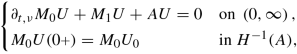
Let H be a Hilbert space, $\mu \in \mathbb {R}$, $M\colon \mathbb {C}_{\operatorname {Re}>\mu }\to L(H)$ a material law, $\nu >\max \{\mathrm {s}_{\mathrm {b}}\left ( M \right ),0\}$ and $A\colon \operatorname {dom}(A)\subseteq H\to H$ skew-selfadjoint. In this section we shall focus on the implementation of initial value problems for evolutionary equations. A priori there is no explicit initial condition implemented in the theory established in $L_{2,\nu }(\mathbb {R};H)$. Indeed, choosing ν > 0 we have only an implicit exponential decay condition at −∞. For initial values at 0, we would rather want to solve the following type of equation. In the situation of the previous section, for a given initial value U ₀ ∈ H we seek to solve the initial value problem

(9.4)

In this generality the initial value problem cannot be solved. Indeed, for $U\in L_{2,\nu }(\mathbb {R};H)$ evaluation at 0 is not well-defined. A way to overcome this difficulty is to weaken the attainment of the initial value. For this, we specialise to the case when

$$\displaystyle \begin{aligned} M(\partial_{t,\nu})=M_{0}+\partial_{t,\nu}^{-1}M_{1} \end{aligned}$$

with M ₀, M ₁ ∈ L(H).

We start with two lemmas, the second of which will also be useful in the next chapter.

Lemma 9.4.1

Let H ₀, H ₁ be Hilbert spaces and assume that H ₁↪H ₀ continuously and densely. Then $C_{\mathrm {c}}^\infty (\mathbb {R};H_1)\subseteq L_{2,\nu }(\mathbb {R};H_1)\cap H_\nu ^1(\mathbb {R};H_0)$ is dense.

Proof

By Proposition 3.2.4, $C_{\mathrm {c}}^\infty (\mathbb {R};H_1)\subseteq H_\nu ^1(\mathbb {R};H_1)$ is dense. Since the embedding $H_\nu ^1(\mathbb {R};H_1)\hookrightarrow L_{2,\nu }(\mathbb {R};H_1)\cap H_\nu ^1(\mathbb {R};H_0)$ is continuous, it thus suffices to show that this embedding is also dense. For this, let $f \in L_{2,\nu }(\mathbb {R};H_1)\cap H_\nu ^1(\mathbb {R};H_0)$. For ε > 0 small enough, we define

By Lemma 9.3.3(b), f _ε → f in $L_{2,\nu }(\mathbb {R};H_1)$ as ε → 0. It remains to show that ∂ _t,ν f _ε → ∂ _t,ν f in $L_{2,\nu }(\mathbb {R};H_0)$ as ε → 0. For this, by definition of $H_\nu ^1(\mathbb {R};H_0)$, we find $g\in L_{2,\nu }(\mathbb {R};H_0)$ such that $f=\partial _{t,\nu }^{-1}g$. Using again Lemma 9.3.3(b), we infer

$$\displaystyle \begin{aligned} \partial_{t,\nu} f_\varepsilon=\partial_{t,\nu}(1+\varepsilon\partial_{t,\nu})^{-1}f = (1+\varepsilon\partial_{t,\nu})^{-1}g \to g = \partial_{t,\nu}f \end{aligned}$$

in $L_{2,\nu }(\mathbb {R};H_0)$ as ε → 0. This concludes the proof. □

Lemma 9.4.2

Let $U_{0}\in \operatorname {dom}(A)$, $U\in L_{2,\nu }(\mathbb {R};H)$ such that is continuous, $\operatorname {\mathrm {spt}} U\subseteq \left [0,\infty \right )$ and

where the first equality is meant in the sense that for all $\varphi \in H_\nu ^{1}(\mathbb {R};H)\cap L_{2,\nu }(\mathbb {R};\operatorname {dom}(A))$ with $\operatorname {\mathrm {spt}}\varphi \subseteq \left [0,\infty \right )$

$$\displaystyle \begin{aligned} \big(\partial_{t,\nu}M_{0}U+M_{1}U+AU\big)(\varphi)=0. \end{aligned}$$

Then and

Proof

We apply Theorem 9.3.2 for showing the claim; that is, we show that

for each $\psi \in H_\nu ^1(\mathbb {R};H)\cap L_{2,\nu }(\mathbb {R};\operatorname {dom}(A))$. Note that by continuity (use Lemma 9.4.1 with H ₀ = H and $H_1=\operatorname {dom}(A)$), it suffices to show the equality for $\psi \in C_{\mathrm {c}}^\infty (\mathbb {R};\operatorname {dom}(A))$. So, let $\psi \in C_{\mathrm {c}}^\infty (\mathbb {R};\operatorname {dom}(A))$ and for $n\in \mathbb {N}$ we define the function $\varphi _n\in H_\nu ^1(\mathbb {R})$ by

Note that $\varphi _n \psi \in H_\nu ^1(\mathbb {R};H)\cap L_{2,\nu }(\mathbb {R};\operatorname {dom}(A))$ and $\operatorname {\mathrm {spt}} (\varphi _n\psi ) \subseteq \left [0,\infty \right )$ for each $n\in \mathbb {N}$. Thus, we obtain

for each $n\in \mathbb {N}$. Thus, the claim follows if we can show that

$$\displaystyle \begin{aligned} \big((\partial_{t,\nu}M_{0}+M_{1}+A)U\big)((1-\varphi_n)\psi)- (\delta_0 M_0 U_0)(\psi)\to 0\quad (n\to \infty). \end{aligned}$$

For doing so, we first observe that for all $n\in \mathbb {N}$ we have

since φ _n(0) = 0. Moreover,

$$\displaystyle \begin{aligned} \big((M_{1}+A)U\big)((1-\varphi_n)\psi)=\left\langle U ,(1-\varphi_n)(M_1^\ast+A^\ast)\psi\right\rangle _{L_{2,\nu}}\to 0\quad (n\to \infty), \end{aligned}$$

since strongly in $L_{2,\nu }(\mathbb {R};H)$ and $\operatorname {\mathrm {spt}} U\subseteq \left [0,\infty \right )$. Thus, it remains to show that

We compute

Note that the last two terms on the right-hand side tend to 0 as n →∞ since, as above, strongly in $L_{2,\nu }(\mathbb {R};H)$ and $\operatorname {\mathrm {spt}} U\subseteq \left [0,\infty \right )$. For the first term, we observe that

by the fundamental theorem of calculus, since (M ₀ U)(t) → M ₀ U ₀ in H ⁻¹(A) as . □

Assume now additionally that there exists c > 0 such that

$$\displaystyle \begin{aligned} zM_0+M_1\geqslant c\quad (z\in \mathbb{C}_{\operatorname{Re}\geqslant \nu}). \end{aligned}$$

Then we can actually prove a stronger result than in the previous lemma.

Theorem 9.4.3

Let $U_{0}\in \operatorname {dom}(A)$, $U\in L_{2,\nu }(\mathbb {R};H)$ . Then the following statements are equivalent:

• (i) is continuous, $\operatorname {\mathrm {spt}} U\subseteq \left [0,\infty \right )$ and

  

  where the first equality is meant as in Lemma 9.4.2.

• (ii) , and we have that .

• (iii) U = S _ν δ ₀ M ₀ U ₀ , with $S_{\nu }\in L(H_{\nu }^{-1}(\mathbb {R};H))$ as in Theorem 9.3.4.

Moreover, in either case we have .

Proof

(i)⇒(ii): This was shown in Lemma 9.4.2.

(ii)⇒(iii): We have that

Applying $\partial _{t,\nu }^{-1}$ to both sides of this equality we infer that

which gives

Applying ∂ _t,ν to both sides and taking into account Theorem 9.3.4, we derive the claim.

(iii)⇒(ii): We do the argument in the proof of (ii)⇒(iii) backwards. First, we apply $\partial _{t,\nu }^{-1}$ to U = S _ν(δ ₀ M ₀ U ₀), which yields

Thus,

An application of ∂ _t,ν yields the claim.

(ii),(iii)⇒(i): Since U = S _ν(δ ₀ M ₀ U ₀), we derive that

$$\displaystyle \begin{aligned} (\partial_{t,\nu}M_0+M_1+A)U\subseteq \delta_0M_0U_0, \end{aligned}$$

which in particular yields (∂ _t,ν M ₀ + M ₁ + A)U = 0 on $\left (0,\infty \right )$. By (ii) we infer

which shows that due to causality and hence, $\operatorname {\mathrm {spt}} U\subseteq \left [0,\infty \right )$. It remains to show that , since this would imply the continuity of with values in H ⁻¹(A) by Theorem 4.1.2 and thus,

since the function is supported on $\left [0,\infty \right )$ only. We compute

and since the right-hand side belongs to $H_\nu ^1(\mathbb {R};H^{-1}(A))$, the assertion follows. □

Remark 9.4.4

By Theorem 9.3.4, we always have $U=S_{\nu }\delta _{0}M_{0}U_{0}\in H_{\nu }^{-1}(\mathbb {R};H)$. This then serves as our generalisation for the initial value problem even if $U_{0}\notin \operatorname {dom}(A)$.

The upshot of Theorem 9.4.3(ii) is that, provided $U_0\in \operatorname {dom}(A)$, we can reformulate initial value problems with the help of our theory as evolutionary equations with L _2,ν-right-hand sides. Thus, we do not need the detour to extrapolation spaces for being able to solve the initial value problem (9.4) (with an adapted initial condition as in (i)) in this situation.

Also note that it may seem that U does depend on the ‘full information’ of U ₀ as it is indicated in (ii). In fact, U only depends on the values of U ₀ orthogonal to the kernel of M ₀ as it is seen in (iii). We conclude this chapter with two examples; the first one is the heat equation, the second example considers Maxwell’s equations.

Example 9.4.5 (Initial Value Problems for the Heat Equation)

We recall the setting for the heat equation outlined in Theorem 6.2.4. This time, we will use homogeneous Dirichlet boundary conditions for the heat distribution θ. Let $\Omega \subseteq \mathbb {R}^{d}$ be open and bounded, a ∈ L _∞( Ω)^d×d with $\operatorname {Re} a(x)\geqslant c>0$ for a.e. x ∈ Ω for some c > 0. In this case, we have

For the unknown heat distribution, θ, we ask it to have the initial value $\theta _{0}\in \operatorname {dom}( \operatorname {\mathrm {grad}}_{0})$. Let ν > 0 and $V\in L_{2,\nu }\big (\mathbb {R};L_2(\Omega )\times L_2(\Omega )^{d}\big )$ be the unique solution of

Then satisfies (ii) from Theorem 9.4.3. Hence, on $\left (0,\infty \right )$ we have

and the initial value is attained in the sense that

which follows from Proposition 9.2.5 where we computed H ⁻¹(A). Let us have a closer look at the attainment of the initial value. As a particular consequence of strong convergence in $H^{-1}( \operatorname {\mathrm {grad}}_{0})$, we obtain for all

as . Since $\operatorname {\mathrm {grad}}_{0}$ is one-to-one and has closed range (see Corollary 11.3.2), we see that has dense and closed range. Hence is onto. This implies that for all ψ ∈ L ₂( Ω)

We deduce that the initial value is attained weakly. This might seem a bit unsatisfactory, however, we shall see stronger assertions for more particular cases in the next chapter.

Next, we have a look at Maxwell’s equations.

Example 9.4.6 (Initial Value Problems for Maxwell’s Equations)

We briefly recall the situation of Maxwell’s equations from Theorem 6.2.8. Let $\varepsilon ,\mu ,\sigma \colon \Omega \to \mathbb {R}^{3\times 3}$ satisfy the assumptions in Theorem 6.2.8 and let $\left (E_{0},H_{0}\right )\in \operatorname {dom}( \operatorname {\mathrm {curl}}_{0})\times \operatorname {dom}( \operatorname {\mathrm {curl}})$. Let $(\widehat {E},\widehat {H})\in L_{2,\nu }(\mathbb {R};L_2(\Omega )^{6})$ satisfy

Then, as we have argued for the heat equation,

satisfies a corresponding initial value problem. We note here that although often the second component in the right-hand side is set to 0, as there are ‘no magnetic monopoles’, in the theory of evolutionary equations the second component of the right-hand side does appear as an initial value in disguise.

9.5 Comments

There are many ways to define spaces generalising the action of an operator to a bigger class of elements; both in a concrete setting and in abstract situations; see e.g. [22, 38]. People have also taken into account simultaneous extrapolation spaces for operators that commute, see e.g. [77, 93].

These spaces are particularly useful for formulating initial value problems as was exemplified above; see also the concluding chapter of [84] for more insight. Yet there is more to it as one can in fact generalise the equation under consideration or even force the attainment of the initial value in a stronger sense. These issues, however, imply that either the initial value is attained in a much weaker sense, or that there are other structural assumptions needed to be imposed on the material law M (as well as on the operator A).

In fact, quite recently, it was established that a particular proper subclass of evolutionary equations can be put into the framework of C ₀-semigroups. The conditions required to allow for statements in this direction are, on the other hand, rather hard to check in practice; see [116, 120].

Exercises

Exercise 9.1

Let H ₀ be a Hilbert space, T ∈ L(H ₀). Compute H ⁻¹(T) and H ⁻¹(T ^∗).

Exercise 9.2

Let H ₀, H ₁ be Hilbert spaces such that H ₀↪H ₁ is dense and continuous. Prove that $H_1^{\prime }\hookrightarrow H_0^{\prime }$ is dense and continuous as well.

Exercise 9.3

Prove the following statement which generalises Proposition 9.2.9 from above: Let H ₀ be a Hilbert space, A ∈ L(H ₀). Assume that $T\colon \operatorname {dom}(T)\subseteq H_{0}\to H_{0}$ is densely defined and closed with 0 ∈ ρ(T) and T ⁻¹ A = AT ⁻¹ + T ⁻¹ BT ⁻¹ for some bounded B ∈ L(H ₀). Then A admits a unique continuous extension, $\overline {{A}}\in L(H^{-1}(T^{*}))$.

Exercise 9.4

Let H ₀ be a Hilbert space, $N\colon \operatorname {dom}(N)\subseteq H_{0}\to H_{0}$ be a normal operator; that is, N is densely defined and closed and NN ^∗ = N ^∗ N. Show that H ⁻¹(N)≅H ⁻¹(N ^∗) and deduce $H^{-1}(\partial _{t,\nu })\cong H^{-1}(\partial _{t,\nu }^{*})$.

Exercise 9.5

Prove Proposition 9.2.8.

Exercise 9.6

Let H ₀ be a Hilbert space, $n\in \mathbb {N}$ and $T\colon \operatorname {dom}(T)\subseteq H_{0}\to H_{0}$ be a densely defined, closed linear operator with 0 ∈ ρ(T). We define and . Show that for all $k\in \mathbb {N}$ and $\ell \in \mathbb {Z}$ we have that H ^k+ℓ(T)↪H ^ℓ(T) continuously and densely. Also show that is dense in H ^ℓ(T) and dense in H ^−ℓ(T ^∗) for all $\ell \in \mathbb {N}$ and that $T|{ }_{\mathcal {D}}$ can be continuously extended to a topological isomorphism H ^ℓ(T) → H ^ℓ−1(T) and to an isomorphism H ^−ℓ+1(T ^∗) → H ^−ℓ(T ^∗) for each $\ell \in \mathbb {N}$.

Exercise 9.7

Prove Lemma 9.3.3.

Hint: Prove a similar equality with $\partial _{t,\nu }^{-1}$ formally replaced by $z\in \partial B\left (r,r\right )\subseteq \mathbb {C}$ and deduce the assertion with the help of Theorem 5.2.3.

References

P. Cojuhari, A. Gheondea, Closed embeddings of Hilbert spaces. J. Math. Anal. Appl. 369(1), 60–75 (2010)
K.-J. Engel, R. Nagel, One-Parameter Semigroups for Linear Evolution Equations, vol. 194. Graduate Texts in Mathematics. With contributions by S. Brendle, M. Campiti, T. Hahn, G. Metafune, G. Nickel, D. Pallara, C. Perazzoli, A. Rhandi, S. Romanelli, R. Schnaubelt (Springer, New York, 2000)
R.S. Palais, Seminar on the Atiyah-Singer Index Theorem. With contributions by M.F. Atiyah, A. Borel, E.E. Floyd, R.T. Seeley, W. Shih, R. Solovay. Annals of Mathematics Studies, vol. 57 (Princeton University Press, Princeton, NJ, 1965)
R. Picard, D. McGhee, Partial Differential Equations: A Unified Hilbert Space Approach, vol. 55. Expositions in Mathematics (DeGruyter, Berlin, 2011)
R. Picard, Evolution equations as operator equations in lattices of Hilbert spaces. Glas. Mat. Ser. III 35(55), 1 (2000). Dedicated to the memory of Branko Najman, pp. 111–136
S. Trostorff, Exponential Stability and Initial Value Problems for Evolutionary Equations. Habilitation Thesis. TU Dresden, 2018
S. Trostorff, Semigroups and evolutionary equations. Semigr. Forum 103(2), 661–699 (2021)
Author information
Authors and Affiliations
Rights and permissions
Open Access This chapter is licensed under the terms of the Creative Commons Attribution 4.0 International License (http://creativecommons.org/licenses/by/4.0/), which permits use, sharing, adaptation, distribution and reproduction in any medium or format, as long as you give appropriate credit to the original author(s) and the source, provide a link to the Creative Commons license and indicate if changes were made.
The images or other third party material in this chapter are included in the chapter's Creative Commons license, unless indicated otherwise in a credit line to the material. If material is not included in the chapter's Creative Commons license and your intended use is not permitted by statutory regulation or exceeds the permitted use, you will need to obtain permission directly from the copyright holder.
Copyright information
© 2022 The Author(s)
About this chapter
Cite this chapter
Seifert, C., Trostorff, S., Waurick, M. (2022). Initial Value Problems and Extrapolation Spaces. In: Evolutionary Equations. Operator Theory: Advances and Applications, vol 287. Birkhäuser, Cham. https://doi.org/10.1007/978-3-030-89397-2_9
Download citation
DOI: https://doi.org/10.1007/978-3-030-89397-2_9
Published:
Publisher Name: Birkhäuser, Cham
Print ISBN: 978-3-030-89396-5
Online ISBN: 978-3-030-89397-2
eBook Packages: Mathematics and StatisticsMathematics and Statistics (R0)