
Abstract
This chapter is devoted to a small tour through a variety of evolutionary equations. More precisely, we shall look into the equations of poro-elastic media, (time-)fractional elasticity, thermodynamic media with delay as well as visco-elastic media. The discussion of these examples will be similar to that of the examples in the previous chapter in the sense that we shall present the equations first, reformulate them suitably and then apply the solution theory to them. The study of visco-elastic media within the framework of partial integro-differential equations will be carried out in the exercises section.
You have full access to this open access chapter, Download chapter PDF
This chapter is devoted to a small tour through a variety of evolutionary equations. More precisely, we shall look into the equations of poro-elastic media, (time-)fractional elasticity, thermodynamic media with delay as well as visco-elastic media. The discussion of these examples will be similar to that of the examples in the previous chapter in the sense that we shall present the equations first, reformulate them suitably and then apply the solution theory to them. The study of visco-elastic media within the framework of partial integro-differential equations will be carried out in the exercises section.
7.1 Poro-Elastic Deformations
In this section we will discuss the equations of poro-elasticity , which form a coupled system of equations. More precisely, the equations of (linearised) elasticity are coupled with the diffusion equation. Before properly writing these equations we introduce the following notation and differential operators.
Definition
Let  be the (closed) subspace of symmetric d × d matrices. Let \(\Omega \subseteq \mathbb {R}^d\) be open. Then define

Analogously, we set  .
.
Note that the symmetry of a d × d matrix here means that the matrix elements are symmetric with respect to the main diagonal. For \(\mathbb {K}=\mathbb {C}\), this does not correspond to the symmetry of the associated linear operator (which would rather be selfadjointness).
Definition
Let \(\Omega \subseteq \mathbb {R}^{d}\) be open. Then we define
and

Similarly to the definitions in the previous chapter, we put  ,
,  and
and  ,
,  , where (analogously to the scalar-valued case) we observe that \( \operatorname {\mathrm {Grad}}_{\mathrm {c}}\subseteq - \operatorname {\mathrm {Div}}_{\mathrm {c}}^{*}\) motivating the notation \( \operatorname {\mathrm {Grad}}\) and \( \operatorname {\mathrm {Grad}}_{0}\).
Remark 7.1.1
Note that in the literature \( \operatorname {\mathrm {Grad}} u\) is also denoted by ε(u) and is called the strain tensor . Due to the (obvious) similarity to the scalar case, we refrain from using ε in this context and prefer \( \operatorname {\mathrm {Grad}}\) instead. Again, the index 0 in the operators refers to generalised Dirichlet (for \( \operatorname {\mathrm {Grad}}_0\)) or Neumann (for \( \operatorname {\mathrm {Div}}_0\)) boundary conditions.
We are now properly equipped to formulate the equations of poro-elasticity ; see also [69] and below for further details. In an elastic body \(\Omega \subseteq \mathbb {R}^{d}\), the displacement field, \(u\colon \mathbb {R}\times \Omega \to \mathbb {R}^{d}\), and the pressure field, \(p\colon \mathbb {R}\times \Omega \to \mathbb {R}\), of a fluid diffusing through Ω satisfy the following two energy balance equations

The right-hand sides \(f\colon \mathbb {R}\times \Omega \to \mathbb {R}^{d}\) and \(g\colon \mathbb {R}\times \Omega \to \mathbb {R}\) describe some given external forcing. We assume homogeneous Neumann boundary conditions for the diffusing fluid as well as homogeneous Dirichlet (i.e. clamped) boundary conditions for the elastic body. The operator ρ ∈ L(L 2( Ω)d) describes the density of the medium Ω (usually realised as a multiplication operator by a bounded, measurable, scalar function). The bounded linear operators \(C\in L(L_2(\Omega )_{\mathrm {sym}}^{d\times d})\) and k ∈ L(L 2( Ω)d) are the elasticity tensor and the hydraulic conductivity of the medium, whereas c 0, λ ∈ L(L 2( Ω)) are the porosity of the medium and the compressibility of the fluid, respectively. The operator α ∈ L(L 2( Ω)) is the so-called Biot–Willis constant. Note that in many applications ρ, c 0, λ and α are just positive real numbers, and C and k are strictly positive definite tensors or matrices.
The reformulation of the equations for poro-elasticity involves several ‘tricks’. One of these is to introduce the matrix trace as the operator

Note that the adjoint is given by \( \operatorname {\mathrm {trace}}^{*}f= \operatorname {\mathrm {diag}}(f,\ldots ,f)\in L_2(\Omega )_{\mathrm {sym}}^{d\times d}\). It is then elementary to obtain  as well as \( \operatorname {\mathrm {grad}}= \operatorname {\mathrm {Div}} \operatorname {\mathrm {trace}}^{*}\). Hence, we formally get

Next, we introduce a new set of unknowns

Here, v is the velocity, T is the stress tensor and q is the heat flux. The quantity ω is an additional variable, which helps to rewrite the system into the form of evolutionary equations.
In order to finalise the reformulation we shall assume some additional properties on the coefficients involved. Throughout the rest of this section, we assume that
for some c > 0, where all inequalities are thought of in the sense of positive definiteness (compare Chap. 6). As a consequence, we obtain

Rewriting the defining equations for T, ω, and q together with the two equations we started out with, we obtain the system

Note that at this stage of modelling we assumed that we can freely interchange the order of differentiation, so that \( \operatorname {\mathrm {Grad}} \partial _t u = \partial _t \operatorname {\mathrm {Grad}} u\). Introducing


we obtain
This perspective enables us to prove well-posedness for the equations of poro-elasticity by applying Theorem 6.2.1.
Theorem 7.1.2
Put
 and let M
0, M
1, V ∈ L(H) and A be given as in (7.1) and (7.2). Then there exists ν
0 > 0 such that for all
\(\nu \geqslant \nu _{0}\)
the operator
\(\overline {\partial _{t,\nu }M_{0}+M_{1}+VAV^{*}}\)
is continuously invertible on
\(L_{2,\nu }(\mathbb {R};H)\)
. The inverse S
ν
of this operator is causal and eventually independent of ν. Moreover,
\(\sup _{\nu \geqslant \nu _{0}}\left \Vert S_{\nu } \right \Vert <\infty \)
and
\(F\in \operatorname {dom}(\partial _{t,\nu })\)
implies
\(S_{\nu }F\in \operatorname {dom}(\partial _{t,\nu })\cap \operatorname {dom}(VAV^{*})\).
and let M
0, M
1, V ∈ L(H) and A be given as in (7.1) and (7.2). Then there exists ν
0 > 0 such that for all
\(\nu \geqslant \nu _{0}\)
the operator
\(\overline {\partial _{t,\nu }M_{0}+M_{1}+VAV^{*}}\)
is continuously invertible on
\(L_{2,\nu }(\mathbb {R};H)\)
. The inverse S
ν
of this operator is causal and eventually independent of ν. Moreover,
\(\sup _{\nu \geqslant \nu _{0}}\left \Vert S_{\nu } \right \Vert <\infty \)
and
\(F\in \operatorname {dom}(\partial _{t,\nu })\)
implies
\(S_{\nu }F\in \operatorname {dom}(\partial _{t,\nu })\cap \operatorname {dom}(VAV^{*})\).
We will provide two prerequisites for the proof. We ask for the details of the proof of Theorem 7.1.2 in Exercise 7.1.
Proposition 7.1.3
Let H 0 , H 1 be Hilbert spaces, \(B\colon \operatorname {dom}(B)\subseteq H_{0}\to H_{0}\) skew-selfadjoint, V ∈ L(H 0, H 1) bijective. Then \(\left (VBV^{*}\right )^{*}=-VBV^{*}\).
The proof of Proposition 7.1.3 is left as (part of) Exercise 7.1.
Proposition 7.1.4
Let H be a Hilbert space, N 0, N 1 ∈ L(H) with \(N_{0}=N_{0}^{*}\) . Assume there exist c 0, c 1 > 0 such that \(\left \langle x ,N_{0}x\right \rangle \geqslant c_{0}\left \Vert x \right \Vert ^{2}\) for all \(x\in \operatorname {ran}(N_0)\) and \(\operatorname {Re}\left \langle y ,N_{1}y\right \rangle \geqslant c_{1}\left \Vert y \right \Vert ^{2}\) for all \(y\in \operatorname {ker}(N_{0})\) . Then for all \(0<c_{1}^{\prime }<c_{1}\) there exists ν 0 > 0 such that for all \(\nu \geqslant \nu _{0}\) we have that
Proof
Note that by the selfadjointness of N 0 we can decompose \(H=\operatorname {\overline {ran}}(N_{0})\oplus \operatorname {ker}(N_{0})\), see Corollary 2.2.6. Let z ∈ H, and \(x\in \operatorname {\overline {ran}}(N_{0})\), \(y\in \operatorname {ker}(N_{0})\) such that z = x + y. For ε, ν > 0 we estimate
where we have used the Peter–Paul inequality (i.e., Young’s inequality for products of non-negative numbers). For \(0<c_{1}^{\prime }<c_{1}\) we find ε > 0 such that \(c_{1}-\varepsilon >c_{1}^{\prime }\). Then we choose \(\nu _{0}>\frac {1}{c_{0}}\left (c_{1}^{\prime }+\frac {1}{\varepsilon }\left \Vert N_{1} \right \Vert ^{2}+\left \Vert N_{1} \right \Vert \right )\). With this choice of ν 0 we deduce for all \(\nu \geqslant \nu _{0}\) that
which yields the assertion. □
7.2 Fractional Elasticity
Let \(\Omega \subseteq \mathbb {R}^d\) be open. In order to better fit to the experimental data of visco-elastic solids (i.e., to incorporate solids that ‘memorise’ previous force applied to them) the equations of linearised elasticity need to be extended in some way. The balance law for the momentum, however, is still satisfied; that is, for the displacement \(u\colon \mathbb {R}\times \Omega \to \mathbb {R}^{d}\) we still have that

where ρ ∈ L(L 2( Ω)d) models the density and \(f\colon \mathbb {R}\times \Omega \to \mathbb {R}^{d}\) is a given external forcing term. The stress tensor , \(T\colon \mathbb {R}\times \Omega \to \mathbb {R}_{\mathrm {sym}}^{d\times d}\), does not follow the classical Hooke’s law, which, if it did, would look like
for \(C\in L(L_2(\Omega )_{\mathrm {sym}}^{d\times d})\). Instead it is amended by another material dependent coefficient \(D\in L(L_2(\Omega )_{\mathrm {sym}}^{d\times d})\) and a fractional time derivative; that is,
for some \(\alpha \in \left [0,1\right ]\), where  , see Example 5.3.1(e). We shall simplify the present consideration slightly and refer to Exercise 7.2 instead for a more involved example. Throughout this section, we shall assume that
for some c > 0. Thus, putting  and assuming the clamped boundary conditions again, we study well-posedness of

In order to do that, we first rewrite the second equation. We will make use of the following proposition which will serve us to show bounded invertibility of \(\partial _t^\alpha \) (in the space L 2,ν), and which will also be employed to obtain well-posedness.
Proposition 7.2.1
Let ν > 0, \(z\in \mathbb {C}_{\operatorname {Re}\geqslant \nu }\) , α ∈ [0, 1]. Then
Proof
Let us prove the first inequality. Note that without loss of generality, we may assume that \(\operatorname {Re} z=1\). Let  . Since \(\ln \circ \cos \) is concave on \(\left (-\tfrac {\pi }{2},\tfrac {\pi }{2}\right )\) (as \((\ln \circ \cos )' = -\tan \) is decreasing) and \((\ln \circ \cos )(0) = 0\), we obtain
and therefore \(\cos {}(\alpha \varphi )\geqslant \cos {}(\varphi )^\alpha \). Since \(\operatorname {Re} z=1\) implies \(\left \vert z \right \vert = \frac {1}{\cos {}(\varphi )}\), we obtain
The second inequality follows from monotonicity of x↦x α. □
Applying Proposition 7.2.1 and noting that D is boundedly invertible we can reformulate (7.4) as

A solution theory for the latter equation, thus, reads as follows, where again  .
.
Theorem 7.2.2
Put
 Then for all ν > 0 the operator

is densely defined and closable in \(L_{2,\nu }(\mathbb {R};H)\) . The inverse of the closure is continuous, causal and eventually independent of ν.
Proof
The proof rests on Theorem 6.2.1. Since \(\begin {pmatrix} 0 & \operatorname {\mathrm {Div}}\\ \operatorname {\mathrm {Grad}}_{0} & 0 \end {pmatrix}\) is skew-selfadjoint by Proposition 6.2.3(a), it suffices to confirm the positive definiteness condition for the material law. For this let \(z\in \mathbb {C}_{\operatorname {Re}\geqslant \nu }\) and compute for \(x\in L_2(\Omega )_{\mathrm {sym}}^{d\times d}\), using Proposition 7.2.1 and Proposition 6.2.3(b),
This yields the assertion. □
7.3 The Heat Equation with Delay
Let \(\Omega \subseteq \mathbb {R}^{d}\) be open. In this section we concentrate on a generalisation of the heat equation discussed in the previous chapter. Although we keep the heat flux balance in the sense that

with \(q\colon \mathbb {R}\times \Omega \to \mathbb {R}^{d}\) being the heat flux and \(\theta \colon \mathbb {R}\times \Omega \to \mathbb {R}\) being the heat, we shall now modify Fourier’s law to the extent that
for some a, b ∈ L(L 2( Ω)d) with \(\operatorname {Re} a\geqslant c\) for some c > 0, and h > 0. We shall again assume homogeneous Neumann boundary conditions for q. Written in the now standard block operator matrix form, this modified heat equation reads

In order to actually justify the existence of the operator \(\left (a+b\tau _{-h}\right )^{-1}\) as a bounded linear operator, we provide the following lemma.
Lemma 7.3.1
Let h > 0.
-
(a)
There exists ν 0 > 0 such that for all \(\nu \geqslant \nu _{0}\) the operator a + bτ −h is continuously invertible on \(L_{2,\nu }(\mathbb {R};L_2(\Omega )^{d})\).
-
(b)
For all \(0<c'<c/\left \Vert a \right \Vert ^{2}\) there is \(\nu _{1}\geqslant \nu _{0}\) such that for all \(z\in \mathbb {C}_{\operatorname {Re}\geqslant \nu _{1}}\) we have \(\operatorname {Re}\left (a+b\mathrm {e}^{-zh}\right )^{-1}\geqslant c'\).
Proof
Note that a is invertible with \(\left \Vert a^{-1} \right \Vert \leqslant \frac {1}{c}\) and \(\operatorname {Re} a^{-1}\geqslant \frac {c}{\left \Vert a \right \Vert ^2}\) by Proposition 6.2.3(b).
-
(a)
By Example 5.3.4(c), for all ν > 0 we obtain
$$\displaystyle \begin{aligned} \left\Vert b\tau_{-h} \right\Vert {}_{L(L_{2,\nu})}\leqslant\left\Vert b \right\Vert {}_{L(L_2(\Omega)^{d})}\sup_{t\in\mathbb{R}}\left\vert \mathrm{e}^{-\left(it+\nu\right)h} \right\vert =\left\Vert b \right\Vert {}_{L(L_2(\Omega)^{d})}\mathrm{e}^{-h\nu}. \end{aligned}$$Thus, we find ν 0 > 0 such that for all \(\nu \geqslant \nu _{0}\) we obtain \(\left \Vert b\tau _{-h}a^{-1} \right \Vert { }_{L(L_{2,\nu })}\leqslant \frac {1}{c}\left \Vert b\tau _{-h} \right \Vert { }_{L(L_{2,\nu })}<1.\) Thus,
$$\displaystyle \begin{aligned} a+b\tau_{-h}=\left(1+b\tau_{-h}a^{-1}\right)a \end{aligned}$$is continuously invertible by a Neumann series argument.
-
(b)
Let \(0<c'<c/\left \Vert a \right \Vert ^{2}\), and set
 . Moreover, we choose \(\nu _{1}\geqslant \nu _{0}\) such that \(\left \Vert d(z) \right \Vert { }_{L(L_2(\Omega )^{d})}\leqslant \min \{\frac {1}{2},\varepsilon \}\) for all \(z\in \mathbb {C}_{\operatorname {Re}\geqslant \nu _{1}}\), where \(0<\varepsilon \leqslant \frac {1}{2}c\left (\frac {c}{\left \Vert a \right \Vert ^{2}}-c'\right )\). For \(z\in \mathbb {C}_{\operatorname {Re}\geqslant \nu _{1}}\) we compute $$\displaystyle \begin{aligned} \operatorname{Re}\left(a+b\mathrm{e}^{-zh}\right)^{-1} & =\operatorname{Re} a^{-1}\left(1-d(z)\right)^{-1} =\operatorname{Re}\left(a^{-1}\sum_{k=0}^{\infty}d(z)^{k}\right) \\ & =\operatorname{Re}\left(a^{-1}+\sum_{k=1}^{\infty}a^{-1}d(z)^{k}\right)\\ & \geqslant\frac{c}{\left\Vert a \right\Vert ^{2}}-\left\Vert \sum_{k=1}^{\infty}a^{-1}d(z)^{k} \right\Vert \geqslant\frac{c}{\left\Vert a \right\Vert ^{2}}-\frac{1}{c}\sum_{k=1}^{\infty}\left\Vert d(z) \right\Vert ^{k}\\ & =\frac{c}{\left\Vert a \right\Vert ^{2}}-\frac{1}{c}\frac{\left\Vert d(z) \right\Vert }{1-\left\Vert d(z) \right\Vert } \geqslant\frac{c}{\left\Vert a \right\Vert ^{2}}-\frac{1}{c}2\varepsilon\geqslant c'. \end{aligned} $$
□
 . Moreover, we choose
 With this lemma we are in the position to provide the well-posedness for the modified heat equation.
Theorem 7.3.2
Let H = L 2( Ω) × L 2( Ω)d . There exists ν 0 > 0 such that for all \(\nu \geqslant \nu _{0}\) the operator

is densely defined and closable with continuously invertible closure on \(L_{2,\nu }(\mathbb {R};H)\) . The inverse of the closure is causal and eventually independent of ν.
Proof
7.4 Dual Phase Lag Heat Conduction
The last example is concerned with a different modification of Fourier’s law. The heat flux balance

is accompanied by the modified Fourier’s law
where \(s_{q}\in \mathbb {R},s_{\theta }>0\) are given numbers, which are called ‘phases’.
Remark 7.4.1
The modified Fourier’s law in (7.6) is an attempt to resolve the problem of infinite propagation speed which stems from a truncated Taylor series expansion of a model given by
Note that it can be shown that such a model would even be ill-posed, see [34].
Let us turn back to the system (7.5) and (7.6). Notice, since s θ > 0, and due to a strictly positive real part of the derivative in our functional analytic setting, we deduce that (1 + s θ ∂ t,ν) is continuously invertible for \(\nu \geqslant 0\). Thus, we obtain
The block operator matrix formulation of the dual phase lag heat conduction model is thus

Theorem 7.4.2
Let H = L 2( Ω) × L 2( Ω)d . Assume \(s_{q}\in \mathbb {R}\setminus \{0\}\) , s θ > 0. Then there exists ν 0 > 0 such that for all \(\nu \geqslant \nu _{0}\) the operator

is densely defined and closable with continuously invertible closure on \(L_{2,\nu }(\mathbb {R};H)\) . The inverse of the closure is causal and eventually independent of ν.
The proof of Theorem 7.4.2 is again based on Theorem 6.2.1. Thus, we shall only record the decisive observation in the next result. For this, we define

Lemma 7.4.3
Let \(s_{q}\in \mathbb {R}\setminus \{0\}, s_{\theta }>0\) . Then there exist \(\nu _{0}\in \mathbb {R}\) and c > 0 such that for all \(z\in \mathbb {C}_{\operatorname {Re}\geqslant \nu _{0}}\) we have
Proof
We put  . Let \(z\in \mathbb {C}\setminus \{0,-\tfrac {1}{s_{\theta }}\}\). We compute
and therefore
By assumption
and since
as \(\operatorname {Re} z\to \infty \), we obtain
for some δ > 0 and all \(z\in \mathbb {C}\) with \(\operatorname {Re} z\) large enough. □
7.5 Comments
The equations of poro-elasticity have been proposed in [69] and were mathematically studied in [63, 103].
Equations of fractional elasticity are discussed in [20, 73, 87, 134]. The well-posedness conditions stated here and in Exercise 7.2 can be generalised as it is outlined in [87] to the case where both C and D are non-negative, selfadjoint operators so that C and D satisfy the conditions imposed on N 1 and N 0 in Proposition 7.1.4. We refrained from presenting this argument here, as it seemed too technical for the time being. Note however that the proof is neither fundamentally different nor considerably less elementary.
The heat equation with delay has also been studied in [55] with an entirely different strategy; the dual phase lag models have been dealt with in [68, 127].
Other ideas to rectify infinite propagation speed of the heat equation can be found in [3], where nonlinear models for heat conduction are being discussed.
The visco-elastic equations discussed in Exercise 7.6 are studied with convolution operators more general than below in [119]; see also [19, 27, 95, 116].
Exercises
Exercise 7.1 (Solutions to the Equations of Poro-Elasticity)
-
(a)
Prove Proposition 7.1.3.
-
(b)
Prove Theorem 7.1.2.
-
(c)
Let \(\Omega \subseteq \mathbb {R}^d\) be open, ν > 0, \(f\in H_{\nu }^{1}(\mathbb {R};L_2(\Omega )^{d})\) and \(g\in H_{\nu }^{1}(\mathbb {R};L_2(\Omega ))\). With the help of Theorem 7.1.2 show that for large enough ν > 0 there exist a unique
 and
and  such that
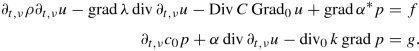
 and
and  such that
Exercise 7.2
Let \(\Omega \subseteq \mathbb {R}^d\) be open, \(C,D\in L(L_2(\Omega )_{\mathrm {sym}}^{d\times d})\), \(D=D^{*}\geqslant c\) for some c > 0 and \(\alpha \in [\tfrac {1}{2},1]\). Show that there exists ν 0 > 0 such that for all \(\nu \geqslant \nu _{0}\) the system

where v = ∂ t,ν u, admits a unique solution \((v,T)\in L_{2,\nu }(\mathbb {R};L_2(\Omega )^{d}\times L_2(\Omega )_{\mathrm {sym}}^{d\times d})\) for all \(f\in H_{\nu }^{1}(\mathbb {R};L_2(\Omega )^{d})\).
The following exercises are devoted to showing the well-posedness of certain equations in visco-elasticity , where the ‘viscous part’ is modelled by convolution with certain integral kernels. The proof of the positive definiteness property requires some preliminary results. We assume the reader to be equipped with the basics from the theory of functions of one complex variable.
For \(U\subseteq \mathbb {C}\) open write  , and for \(u\colon U\to \mathbb {C}\) holomorphic, define \(f_{\operatorname {Re}\,u}\colon \widetilde {U}\to \mathbb {R}\) by
  for \((x,y)\in \widetilde {U}\). We put

Exercise 7.3
Let \(U\subseteq \mathbb {C}\) be open.
-
(a)
Let \(f\in H_{\operatorname {Re}}(U)\). Show that f satisfies the mean value property ; that is, for all \((x,y)\in \widetilde {U}\) and r > 0 with \(\overline {B\left ((x,y),r\right )}\subseteq \widetilde {U}\) we have
$$\displaystyle \begin{aligned} f(x,y)=\frac{1}{2\pi}\int_{0}^{2\pi}f(x+r\cos\theta,y+r\sin\theta)\,\mathrm{d}\theta. \end{aligned}$$ -
(b)
Let
 and \(f\in H_{\operatorname {Re}}(U)\cap C(\mathbb {R}\times \mathbb {R}_{\geqslant 0})\). Moreover, assume that f(x, 0) = 0 for each \(x\in \mathbb {R}\) and f(x, y) → 0 as |(x, y)|→∞. Show that f = 0 on \(\mathbb {R}\times \mathbb {R}_{\geqslant 0}\).
 and
and Exercise 7.4
In this exercise we show a version of
Poisson’s formula
. Let  and \(f\in H_{\operatorname {Re}}(U)\cap C(\mathbb {R}\times \mathbb {R}_{\geqslant 0})\).
-
(a)
Assume that \(f(\cdot ,0)\in L_p(\mathbb {R})\) for some \(1\leqslant p<\infty \). Show that \(\mathbb {C}_{\operatorname {Im}>0}\ni z\mapsto \frac {1}{\pi }\int _{\mathbb {R}}\frac {\operatorname {Im} z'+\mathrm {i}\left (\operatorname {Re} z-x'\right )}{(\operatorname {Re} z-x')^{2}+(\operatorname {Im} z)^{2}}f(x',0)\,\mathrm {d} x'\) is holomorphic.
-
(b)
Assume that \(f(\cdot ,0)\in L_\infty (\mathbb {R})\). Show that \(\frac {1}{\pi } \int _{\mathbb {R}} \frac {y}{(x-x')^2+y^2)} f(x',0)\,\mathrm {d} x'\to f(x_0,0)\) as x → x 0 and
 .
. -
(c)
(Poisson’s formula) Assume that \(f(\cdot ,0)\in L_p(\mathbb {R})\) for some \(1\leqslant p<\infty \) and f(x, y) → 0 as |(x, y)|→∞ in \(\mathbb {R}\times \mathbb {R}_{\geqslant 0}\). Show that
$$\displaystyle \begin{aligned} f(x,y)=\frac{1}{\pi}\int_{\mathbb{R}}\frac{y}{(x-x')^{2}+y^{2}}f(x',0)\,\mathrm{d} x'\quad ((x,y)\in \mathbb{R}\times \mathbb{R}_{>0}). \end{aligned}$$
 .
.Exercise 7.5
Let \(\nu _{0}\in \mathbb {R}\) and \(k\in L_{1,\nu _{0}}(\mathbb {R};\mathbb {R})\) with \( \operatorname {\mathrm {spt}} k\subseteq \mathbb {R}_{\geqslant 0}\).
-
(a)
Show that for all \((x,\nu )\in \mathbb {R}\times \mathbb {R}_{>{\nu _{0}}}\) we have
$$\displaystyle \begin{aligned} \operatorname{Im}(\mathcal{L}k)(\mathrm{i} x+\nu)=\frac{1}{\pi}\int_{\mathbb{R}}\frac{\nu-\nu_{0}}{(x-x')^{2}+(\nu-\nu_{0})^{2}}\operatorname{Im}(\mathcal{L}k)(\mathrm{i} x'+\nu_{0})\,\mathrm{d} x'. \end{aligned}$$Hint: Approximate k by functions in \(C_{\mathrm {c}}^\infty (\mathbb {R}_{\geqslant 0};\mathbb {R})\) and use Poisson’s formula (see Exercise 7.4).
-
(b)
Assume there exists d⩾0 such that for all \(x\in \mathbb {R}\)
$$\displaystyle \begin{aligned} x\operatorname{Im}(\mathcal{L}k)(\mathrm{i} x+\nu_{0})\leqslant d. \end{aligned}$$Show that for all \(\nu \geqslant \nu _{0}\) and \(x\in \mathbb {R}\) we have
$$\displaystyle \begin{aligned} x\operatorname{Im}(\mathcal{L}k)(\mathrm{i} x+\nu)\leqslant4d. \end{aligned}$$Hint: Use the formula in (a) and split the integral into positive and negative part of \(\mathbb {R}\); use symmetry of \((\mathcal {L}k)\) under conjugation due to the realness of k.
Exercise 7.6
Let \(\Omega \subseteq \mathbb {R}^{d}\) be open, \(\nu _{0}\in \mathbb {R}\) and \(k\in L_{1,\nu _{0}}(\mathbb {R};\mathbb {R})\) with \( \operatorname {\mathrm {spt}} k\subseteq \mathbb {R}_{\geqslant 0}\). Assume there exists d⩾0 such that
Show that there exists \(\nu _{1}\geqslant \nu _{0}\) such that for all \(\nu \geqslant \nu _1\) the operator

is well-defined, densely defined and closable in \(L_{2,\nu }(\mathbb {R};H)\) with \(H=L_2(\Omega )^{d}\times L_2(\Omega )_{\mathrm {sym}}^{d\times d}\). Further, show that its closure is continuously invertible, and that the corresponding inverse is causal and eventually independent of ν.
Exercise 7.7
Let \(\nu _{0}\in \mathbb {R}\) and \(k\in L_{1,\nu _{0}}(\mathbb {R};\mathbb {R})\) with \( \operatorname {\mathrm {spt}} k\subseteq \mathbb {R}_{\geqslant 0}\).
-
(a)
Assume that k is absolutely continuous with \(k'\in L_{1,\nu _{0}}(\mathbb {R};\mathbb {R})\). Show that there exist \(\nu _{1}\geqslant \nu _{0}\) and d⩾0 with
$$\displaystyle \begin{aligned} x\operatorname{Im}(\mathcal{L}k)(\mathrm{i} x+\nu_{1})\leqslant d\quad (x\in\mathbb{R}). \end{aligned}$$ -
(b)
Assume that k(t)⩾0 for all \(t\in \mathbb {R}\) and that \(k(t)\leqslant k(s)\), whenever \(s\leqslant t\). Show that there exists \(\nu _{1}\geqslant \nu _{0}\) with
$$\displaystyle \begin{aligned} x\operatorname{Im}(\mathcal{L}k)(\mathrm{i} x+\nu_{1})\leqslant 0\quad (x\in\mathbb{R}). \end{aligned}$$Hint: For part (b) use the explicit formula for \(\operatorname {Im} (\mathcal {L}k)\) as an integral and the periodicity of \(\sin \).
Remark: The condition in (a) is a standard assumption for convolution kernels in the framework of visco-elastic equations; the condition in (b) is from [95].
References
F. Andreu et al., Finite propagation speed for limited flux diffusion equations. Arch. Ration. Mech. Anal. 182(2), 269 (2006)
P. Cannarsa, D. Sforza, Global solutions of abstract semilinear parabolic equations with memory terms. Nonlinear Differ. Equ. Appl. 10(4), 399–430 (2003)
K. Cherednichenko, M. Waurick, Resolvent estimates in homogenisation of periodic problems of fractional elasticity. J. Differ. Equ. 264(6), 3811–3835 (2018)
C.M. Dafermos, An abstract Volterra equation with applications to linear viscoelasticity. J. Differ. Equ. 7, 554–569 (1970)
M. Dreher, R. Quintanilla, R. Racke, Ill-posed problems in thermomechanics. Appl. Math. Lett. 22(9), 1374–1379 (2009)
D. Khusainov, M. Pokojovy, R. Racke, Strong and mild extrapolated L 2- solutions to the heat equation with constant delay. SIAM J. Math. Anal. 47(1), 427–454 (2015)
D.F. McGhee, R. Picard, A note on anisotropic, inhomogeneous, poro-elastic media. Math. Methods Appl. Sci. 33(3), 313–322 (2010)
S. Mukhopadyay et al., On some models in linear thermo-elasticity with rational material laws. Math. Mech. Solids 21(9), 1149–1163 (2016)
M.A. Murad, J.H. Cushman, Multiscale flow and deformation in hydrophilic swelling porous media. Int. J. Eng. Sci. 34(3), 313–338 (1996)
B. Nolte, S. Kempfle, I. Schäfer, Does a real material behave fractionally? Applications of fractional differential operators to the damped structure borne sound in viscoelastic solids. J. Comput. Acoust. 11(03), 451–489 (2003). eprint: https://doi.org/10.1142/S0218396X03002024
R. Picard, S. Trostorff, M. Waurick, On evolutionary equations with material laws containing fractional integrals. Math. Method Appl. Sci. 38(15), 3141–3154 (2015)
J. Prüss, Decay properties for the solutions of a partial differential equation with memory. Archiv der Mathematik 92(2), 158–173 (2009)
R.E. Showalter, Diffusion in poro-elastic media. J. Math. Anal. Appl. 251(1), 310–340 (2000)
S. Trostorff, Exponential Stability and Initial Value Problems for Evolutionary Equations. Habilitation Thesis. TU Dresden, 2018
S. Trostorff, On integro-differential inclusions with operator-valued kernels. Math. Method Appl. Sci. 38(5), 834–850 (2015)
D. Tzou, A unified field approach for heat conduction from macro-to microscales. J. Heat Transfer 117(1), 8–16 (1995)
M. Waurick, Homogenization in fractional elasticity. SIAM J. Math. Anal. 46(2), 1551–1576 (2014)
Author information
Authors and Affiliations
Rights and permissions
Open Access This chapter is licensed under the terms of the Creative Commons Attribution 4.0 International License (http://creativecommons.org/licenses/by/4.0/), which permits use, sharing, adaptation, distribution and reproduction in any medium or format, as long as you give appropriate credit to the original author(s) and the source, provide a link to the Creative Commons license and indicate if changes were made.
The images or other third party material in this chapter are included in the chapter's Creative Commons license, unless indicated otherwise in a credit line to the material. If material is not included in the chapter's Creative Commons license and your intended use is not permitted by statutory regulation or exceeds the permitted use, you will need to obtain permission directly from the copyright holder.
Copyright information
© 2022 The Author(s)
About this chapter

Cite this chapter
Seifert, C., Trostorff, S., Waurick, M. (2022). Examples of Evolutionary Equations. In: Evolutionary Equations. Operator Theory: Advances and Applications, vol 287. Birkhäuser, Cham. https://doi.org/10.1007/978-3-030-89397-2_7
Download citation
DOI: https://doi.org/10.1007/978-3-030-89397-2_7
Published:
Publisher Name: Birkhäuser, Cham
Print ISBN: 978-3-030-89396-5
Online ISBN: 978-3-030-89397-2
eBook Packages: Mathematics and StatisticsMathematics and Statistics (R0)