Maximal Regularity

Abstract

In this chapter, we address the issue of maximal regularity. More precisely, we provide a criterion on the ‘structure’ of the evolutionary equation

$$\displaystyle \left (\overline {\partial _{t,\nu }M(\partial _{t,\nu })+A}\right )U=F $$

in question and the right-hand side F in order to obtain $U\in \operatorname {dom}(\partial _{t,\nu }M(\partial _{t,\nu }))\cap \operatorname {dom}(A)$. If $F\in L_{2,\nu }(\mathbb {R};H)$, $U\in \operatorname {dom}(\partial _{t,\nu }M(\partial _{t,\nu }))\cap \operatorname {dom}(A)$ is the optimal regularity one could hope for. However, one cannot expect U to be as regular since $\left (\partial _{t,\nu }M(\partial _{t,\nu })+A\right )$ is simply not closed in general. Hence, in all the cases where $\left (\partial _{t,\nu }M(\partial _{t,\nu })+A\right )$ is not closed, the desired regularity property does not hold for $F\in L_{2,\nu }(\mathbb {R};H)$. However, note that by Picard’s theorem, $F\in \operatorname {dom}(\partial _{t,\nu })$ implies the desired regularity property for U given the positive definiteness condition for the material law is satisfied and A is skew-selfadjoint. In this case, one even has $U\in \operatorname {dom}(\partial _{t,\nu })\cap \operatorname {dom}(A)$, which is more regular than expected. Thus, in the general case of an unbounded, skew-selfadjoint operator A neither the condition $F\in \operatorname {dom}(\partial _{t,\nu })$ nor $F\in L_{2,\nu }(\mathbb {R};H)$ yields precisely the regularity $U\in \operatorname {dom}(\partial _{t,\nu }M(\partial _{t,\nu }))\cap \operatorname {dom}(A)$ since

$$\displaystyle \operatorname {dom}(\partial _{t,\nu })\cap \operatorname {dom}(A)\subseteq \operatorname {dom}(\partial _{t,\nu }M(\partial _{t,\nu }))\cap \operatorname {dom}(A)\subseteq \operatorname {dom}(\overline {\partial _{t,\nu }M(\partial _{t,\nu })+A}), $$

where the inclusions are proper in general. It is the aim of this chapter to provide an example case, where less regularity of F actually yields more regularity for U. If one focusses on time-regularity only, this improvement of regularity is in stark contrast to the general theory developed in the previous chapters. Indeed, in this regard, one can coin the (time) regularity asserted in Picard’s theorem as “U is as regular as F”. For a more detailed account on the usual perspective of maximal regularity (predominantly) for parabolic equations, we refer to the Comments section of this chapter.

In this chapter, we address the issue of maximal regularity. More precisely, we provide a criterion on the ‘structure’ of the evolutionary equation

$$\displaystyle \begin{aligned} \left(\overline{\partial_{t,\nu}M(\partial_{t,\nu})+A}\right)U=F \end{aligned}$$

in question and the right-hand side F in order to obtain $U\in \operatorname {dom}(\partial _{t,\nu }M(\partial _{t,\nu }))\cap \operatorname {dom}(A)$. If $F\in L_{2,\nu }(\mathbb {R};H)$, $U\in \operatorname {dom}(\partial _{t,\nu }M(\partial _{t,\nu }))\cap \operatorname {dom}(A)$ is the optimal regularity one could hope for. However, one cannot expect U to be as regular since $\left (\partial _{t,\nu }M(\partial _{t,\nu })+A\right )$ is simply not closed in general. Hence, in all the cases where $\left (\partial _{t,\nu }M(\partial _{t,\nu })+A\right )$ is not closed, the desired regularity property does not hold for $F\in L_{2,\nu }(\mathbb {R};H)$. However, note that by Picard’s theorem, $F\in \operatorname {dom}(\partial _{t,\nu })$ implies the desired regularity property for U given the positive definiteness condition for the material law is satisfied and A is skew-selfadjoint. In this case, one even has $U\in \operatorname {dom}(\partial _{t,\nu })\cap \operatorname {dom}(A)$, which is more regular than expected. Thus, in the general case of an unbounded, skew-selfadjoint operator A neither the condition $F\in \operatorname {dom}(\partial _{t,\nu })$ nor $F\in L_{2,\nu }(\mathbb {R};H)$ yields precisely the regularity $U\in \operatorname {dom}(\partial _{t,\nu }M(\partial _{t,\nu }))\cap \operatorname {dom}(A)$ since

$$\displaystyle \begin{aligned} \operatorname{dom}(\partial_{t,\nu})\cap\operatorname{dom}(A)\subseteq\operatorname{dom}(\partial_{t,\nu}M(\partial_{t,\nu}))\cap\operatorname{dom}(A)\subseteq \operatorname{dom}(\overline{\partial_{t,\nu}M(\partial_{t,\nu})+A}), \end{aligned}$$

where the inclusions are proper in general. It is the aim of this chapter to provide an example case, where less regularity of F actually yields more regularity for U. If one focusses on time-regularity only, this improvement of regularity is in stark contrast to the general theory developed in the previous chapters. Indeed, in this regard, one can coin the (time) regularity asserted in Picard’s theorem as “U is as regular as F”. For a more detailed account on the usual perspective of maximal regularity (predominantly) for parabolic equations, we refer to the Comments section of this chapter.

15.1 Guiding Examples and Non-Examples

Before we present the abstract theory, we motivate the general setting looking at a particular example. Traditionally, in the discussion of partial differential equations and their classification, people focus on regularity theory. Thus, one finds the non-exhaustive categories ‘elliptic’, ‘parabolic’, and ‘hyperbolic’. Since we do not want to dive into the intricacies of this classification much less their regularity, we only name some examples of the said subclasses. Laplace’s equation from Chap. 1 falls into the class of elliptic PDEs, the heat equation is a paradigm example of a parabolic equation and Maxwell’s equations or the transport equation are hyperbolic.

Since we predominantly treat time-dependent equations and elliptic PDEs usually are time-independent, we only look at examples for hyperbolic and parabolic equations more closely. As for the hyperbolic case, we consider the transport equation next and highlight that any ‘gain’ in regularity as hinted at in the introduction of this chapter is not possible.

Example 15.1.1

We define $\partial \colon H^{1}(\mathbb {R})\subseteq L_2(\mathbb {R})\to L_2(\mathbb {R}),\phi \mapsto \phi '$. Then, by Corollary 3.2.6, ∂ ^∗ = −∂; that is, ∂ is skew-selfadjoint. We consider for ν > 0 the operator

$$\displaystyle \begin{aligned} \partial_{t,\nu}+\partial \end{aligned}$$

in $L_{2,\nu }(\mathbb {R};L_2(\mathbb {R}))$. Then, by Picard’s theorem, $0\in \rho \big (\overline {\partial _{t,\nu }+\partial }\big )$; that is, $\big (\overline {\partial _{t,\nu }+\partial }\big )^{-1}\in L(L_{2,\nu }(\mathbb {R};L_2(\mathbb {R})))$. Next, consider the functions

for some $h\in L_2(\mathbb {R})$. Then it is not difficult to see that $u,f\in L_{2,\nu }(\mathbb {R};L_2(\mathbb {R})).$ If $h\in C_{\mathrm {c}}^\infty (\mathbb {R})$, then

$$\displaystyle \begin{aligned} u\in H_{\nu}^{1}(\mathbb{R};H^{1}(\mathbb{R}))\subseteq\operatorname{dom}(\partial_{t,\nu}+\partial) \end{aligned}$$

and

$$\displaystyle \begin{aligned} (\partial_{t,\nu}+\partial)u=f. \end{aligned}$$

If $h\in L_2(\mathbb {R})\setminus H^{1}(\mathbb {R})$, then one can show that $u\in \operatorname {dom}\big (\overline {\partial _{t,\nu }+\partial }\big )$, $\big (\overline {\partial _{t,\nu }+\partial }\big )u=f$ and

$$\displaystyle \begin{aligned} u\notin\operatorname{dom}(\partial_{t,\nu})\cap\operatorname{dom}(\partial). \end{aligned}$$

For this observation, we refer to Exercise 15.1. Thus, being in the domain of $\overline {\partial _{t,\nu }+\partial }$ does not necessarily imply being in the domain of either $\operatorname {dom}(\partial _{t,\nu })$ or $\operatorname {dom}(\partial )$.

The last example has shown that we cannot expect an improvement of regularity for the considered transport equation. In fact, it is possible to provide an example of a similar type for the wave equation (and similar hyperbolic type equations including Maxwell’s equations). Thus, in order to have an improvement of regularity one needs to further restrict the class of evolutionary equations. We now provide a guiding example, where we discuss an abstract variant of the heat equation.

Example 15.1.2

Let ℓ ₂ be the space of square summable sequences indexed by $n\in \mathbb {N}$. We note that ℓ ₂ is isomorphic to $L_2(\#_{\mathbb {N}})$, where $\#_{\mathbb {N}}$ is the counting measure on $\mathbb {N}$. We introduce $\mathrm {m}\colon \operatorname {dom}(\mathrm {m})\subseteq \ell _{2} \to \ell _{2}$ the operator of multiplying by the argument. Then, m is an unbounded, selfadjoint operator. Next, we consider the operator

$$\displaystyle \begin{aligned} \partial_{t,\nu}\begin{pmatrix} 1 & 0\\ 0 & 0 \end{pmatrix}+\begin{pmatrix} 0 & 0\\ 0 & 1 \end{pmatrix}+\begin{pmatrix} 0 & -\mathrm{m}\\ \mathrm{m} & 0 \end{pmatrix} \end{aligned}$$

on $L_{2,\nu }(\mathbb {R};\ell _{2})$. Then, Picard’s theorem applies and we obtain

$$\displaystyle \begin{aligned} 0\in\rho\left(\overline{\partial_{t,\nu}\begin{pmatrix} 1 & 0\\ 0 & 0 \end{pmatrix}+\begin{pmatrix} 0 & 0\\ 0 & 1 \end{pmatrix}+\begin{pmatrix} 0 & -\mathrm{m}\\ \mathrm{m} & 0 \end{pmatrix}}\right). \end{aligned}$$

For $f\in L_{2,\nu }(\mathbb {R};\ell _{2})$ define

Then $u\in \operatorname {dom}(\partial _{t,\nu })\cap \operatorname {dom}(\mathrm {m})$ and $q\in \operatorname {dom}(\mathrm {m})$. We ask the reader to fill in the details in Exercise 15.2.

Remark 15.1.3

The last example is in fact an abstract version of the heat equation on bounded domains. We refer to [90, Section 2.2.2] for a corresponding reasoning for the Schrödinger equation.

Let us compare the two different examples, the transport equation and the abstract parabolic equation. From the perspective of evolutionary equations; that is, looking at equations of the form

$$\displaystyle \begin{aligned} (\partial_{t,\nu}M_{0}+M_{1}+A)U=F, \end{aligned}$$

for the transport equation we have M ₀ = 1 and M ₁ = 0. In the case of the abstract parabolic equation, M ₀ has a nontrivial kernel, which is compensated in M ₁. Moreover, the decomposition of kernel and range of M ₀ is comparable to the block structure of A. Thus, we may hope for an improvement of regularity as in Example 15.1.2 if these abstract conditions are met. This observation is the starting point of parabolic evolutionary pairs to be defined in the next section.

15.2 The Maximal Regularity Theorem and Fractional Sobolev Spaces

In order to be able to formulate the main theorem of this chapter, we need the notion of fractional Sobolev spaces. For this, we recall from Example 5.3.4 and Sect. 7.2 that we already dealt with fractional powers of the time-derivative. For α, ν≥ 0, we thus consistently define

with maximal domain in $L_{2,\nu }(\mathbb {R};H)$, where we agree with setting . Note that in this case, using Proposition 7.2.1, $0\in \rho (\partial _{t,\nu }^\alpha )$ given ν > 0. Hence, the following construction yields Hilbert spaces; for this also recall that $\left \langle \cdot ,\cdot \right \rangle _A$ denotes the graph inner product of a linear operator A defined in a Hilbert space.

Definition

Let α, ν ≥ 0. Then we define

for ν > 0 and

Lemma 15.2.1

For all α, ν ≥ 0 the space $H_{\nu }^{\alpha }(\mathbb {R};H)$ is a Hilbert space. Moreover, $H_{\nu }^{\alpha }(\mathbb {R};H)\hookrightarrow L_{2,\nu }(\mathbb {R};H)$ continuously and densely.

Proof

We only show the claim for ν > 0. By Fourier–Laplace transformation, the claim follows if we show that

$$\displaystyle \begin{aligned} (\mathrm{i}\mathrm{m}+\nu)^\alpha \colon \operatorname{dom}((\mathrm{i}\mathrm{m}+\nu)^\alpha)\subseteq L_2(\mathbb{R};H)\to L_2(\mathbb{R};H) \end{aligned}$$

is densely defined and continuously invertible. For this, we find $n\in \mathbb {N}$ and $\beta \in \left [0,1\right )$ such that α = n + β. It is easy to see that (im + ν)^α = (im + ν)ⁿ(im + ν)^β. Thus, continuous invertibility readily follows from the continuous invertibility of (im + ν) and (im + ν)^β (for the latter, see also Proposition 7.2.1). For the case when $H=\mathbb {K}$, it follows from Theorem 2.4.3 that (im + ν)^α is densely defined. Thus, it follows from Lemma 3.1.8 that (im + ν)^α is densely defined also for general H. □

In order to state our main theorem, we introduce the notion of parabolic pairs.

Definition

Let $M\colon \operatorname {dom}(M)\subseteq \mathbb {C}\to L(H)$ be a material law, $A\colon \operatorname {dom}(A)\subseteq H\to H$ and α ∈ (0, 1]. We call (M, A) an (α-)fractional parabolic pair if the following conditions are met: there exist $\nu >\max \{0,\mathrm {s}_{\mathrm {b}}\left ( M \right )\}$ and c > 0 such that

$$\displaystyle \begin{aligned} \operatorname{Re} zM(z)\geqslant c\quad (z\in\mathbb{C}_{\operatorname{Re}>\nu}), \end{aligned}$$

and moreover, we find a closed subspace H ₀ ⊆ H, $C\colon \operatorname {dom}(C)\subseteq H_{0}\to H_{1}$ closed and densely defined, and $M_{00}\in \mathcal {M}(H_{0};\nu )$, $N\in \mathcal {M}(H;\nu )$ such that

$$\displaystyle \begin{aligned} M(z)=\begin{pmatrix} M_{00}(z) & 0\\ 0 & 0 \end{pmatrix}+z^{-1}N(z),\quad A=\begin{pmatrix} 0 & -C^{*}\\ C & 0 \end{pmatrix}, \end{aligned}$$

and

$$\displaystyle \begin{aligned} & \operatorname{Re} z^{1-\alpha}M_{00}(z)\geqslant c'\quad (z\in\mathbb{C}_{\operatorname{Re}>\nu}) \end{aligned} $$

for some c′ > 0, and $\mathbb {C}_{\operatorname {Re}>\nu }\ni z\mapsto z^{1-\alpha }M_{00}(z)\in L(H_0)$ is bounded. A 1-fractional parabolic pair is called parabolic .

Remark 15.2.2

• (a) If (M, A) is α-fractional parabolic and β-fractional parabolic with the same decomposition H = H ₀ ⊕ H ₁, then α = β. Indeed, assume that α < β. Then

  $$\displaystyle \begin{aligned} z^{1-\beta}M_{00}(z)=z^{\alpha-\beta}z^{1-\alpha}M_{00}(z)\to0\quad (|z|\to\infty,z\in\mathbb{C}_{\operatorname{Re}>\nu}) \end{aligned}$$

  contradicting the real-part condition.

• (b) If (M, A) is α-fractional parabolic, then there exists μ > ν such that for all $z\in \mathbb {C}_{\operatorname {Re}>\mu }$

  $$\displaystyle \begin{aligned} \operatorname{Re} z^{1-\alpha}\left(M_{00}(z)+z^{-1}N_{00}(z)\right)\geqslant c'/2\quad \end{aligned} $$

  (15.1)

  for some c′ > 0, where . Indeed, this follows from the fact that z ^−α N ₀₀(z) → 0 as $\operatorname {Re} z\to \infty$.

The main theorem of this chapter is the following:

Theorem 15.2.3

Let α ∈ (0, 1] and (M, A) be α-fractional parabolic (with H = H ₀ ⊕ H ₁ and C from H ₀ to H ₁ ) and assume that (15.1) holds for all $z\in \mathbb {C}_{\mathit{\mbox{Re}} >\nu }$ for some $\nu >\max \{0,\mathrm {s}_{\mathrm {b}}\left ( M \right )\}$ . Let $f\in L_{2,\nu }(\mathbb {R};H_{0})$ and $g\in H_{\nu }^{\alpha /2}(\mathbb {R};H_{1})$ . Then the solution satisfies

$$\displaystyle \begin{aligned} u & \in H_{\nu}^{\alpha}(\mathbb{R};H_{0})\cap H_{\nu}^{\alpha/2}\big(\mathbb{R};\operatorname{dom}(C)\big)\\ v & \in H_{\nu}^{\alpha/2}(\mathbb{R};H_{1})\cap L_{2,\nu}\big(\mathbb{R};\operatorname{dom}(C^{*})\big). \end{aligned} $$

More precisely,

$$\displaystyle \begin{aligned} \begin{array}{rcl} & &\displaystyle \big(\overline{\partial_{t,\nu}M(\partial_{t,\nu})+A}\big)^{-1}\colon L_{2,\nu}(\mathbb{R};H_{0})\oplus H_{\nu}^{\alpha/2}(\mathbb{R};H_{1})\\ & &\displaystyle \qquad \qquad \quad \to\big(H_{\nu}^{\alpha}(\mathbb{R};H_{0})\cap H_{\nu}^{\alpha/2}\big(\mathbb{R};\operatorname{dom}(C)\big)\big)\oplus\big(H_{\nu}^{\alpha/2}(\mathbb{R};H_{1})\cap L_{2,\nu}\big(\mathbb{R};\operatorname{dom}(C^{*})\big)\big) \end{array} \end{aligned} $$

is continuous.

Example 15.2.4 (Heat Equation)

Let us recall the heat equation from Theorem 6.2.4. For $\Omega \subseteq \mathbb {R}^d$ open, we let a ∈ L(L ₂( Ω)^d) such that

$$\displaystyle \begin{aligned} \operatorname{Re} a \geqslant c \end{aligned}$$

in the sense of positive definiteness. It is not difficult to see that

is parabolic; with the obvious orthogonal decomposition of the underlying Hilbert space. Let $f\in L_{2,\nu }(\mathbb {R};L_2(\Omega ))$. Then

particularly satisfies the regularity statement

The next example deals with a parabolic variant of the equations introduced in (7.3) and (7.4) describing fractional elasticity. We modify the equations at hand by considering $\alpha \in \left [1,2\right ]$.

Example 15.2.5 (Parabolic Fractional Viscoelasticity)

Let $\Omega \subseteq \mathbb {R}^d$ open and recall the differential operators $\operatorname {\mathrm {Div}}$ and $\operatorname {\mathrm {Grad}}_0$ from Sect. 7.1 defined in the spaces $L_2(\Omega )_{\mathrm {sym}}^{d\times d}$ and L ₂( Ω)^d, respectively. Let c > 0 and $D\in L\big (L_2(\Omega )_{\mathrm {sym}}^{d\times d}\big )$, ρ = ρ ^∗∈ L(L ₂( Ω)^d). For ν > 0 and $f\in L_{2,\nu }(\mathbb {R}; L_2(\Omega )^d)$ consider the problem of finding $u\colon \mathbb {R}\times \Omega \to \mathbb {R}^d$ such that

(15.2)

$$\displaystyle \begin{aligned} T & = D\partial_{t,\nu}^\alpha \operatorname{\mathrm{Grad}}_0 u, \end{aligned} $$

(15.3)

for some $\alpha \in \left [1,2\right )$, where $\rho \geqslant c$ and $\operatorname {Re} D\geqslant c$ in the sense of positive definiteness. We rewrite the system just introduced by using to (formally) obtain

Note that . Thus, using the selfadjointness and positive definiteness of ρ as well as Proposition 7.2.1, we infer

$$\displaystyle \begin{aligned} \operatorname{Re} (z^\gamma \rho) \geqslant \nu^\gamma c\quad (z\in \mathbb{C}_{\operatorname{Re}\geqslant \nu}). \end{aligned}$$

Consequently, applying Proposition 6.2.3(b) to a = D, we get that

is γ-fractional parabolic. In consequence, the solution (v, T) of

additionally satisfies the following regularity properties

Rephrasing this for $u=\partial _{t,\nu }^{-\alpha }v$, we even have

$$\displaystyle \begin{aligned} u\in H_\nu^2\big(\mathbb{R};L_2(\Omega)^d\big)\cap H_\nu^{1+\alpha/2}\big(\mathbb{R};\operatorname{dom}( \operatorname{\mathrm{Grad}}_0)\big), \end{aligned}$$

which, since $\alpha /2 \leqslant 1$, particularly implies that the equations (15.2) and (15.3) are equalities valid in $L_{2,\nu }\big (\mathbb {R};L_2(\Omega )^d\big )$ and $L_{2,\nu }\big (\mathbb {R};L_2(\Omega )_{\mathrm {sym}}^{d\times d}\big )$, respectively.

15.3 The Proof of Theorem 15.2.3

The decisive estimate in connection to the proof of Theorem 15.2.3 is contained in the following statement. For the entire rest of the section, we shall denote the norm and scalar product in $H_\nu ^\alpha (\mathbb {R};K)$, K some Hilbert space, by ∥⋅∥_α and $\left \langle \cdot ,\cdot \right \rangle _\alpha$, respectively.

Lemma 15.3.1

Let H ₀, H ₁ be Hilbert spaces, $C\colon \operatorname {dom}(C)\subseteq H_{0}\to H_{1}$ densely defined and closed. Let α ∈ [0, 1], $M_{j}\colon \operatorname {dom}(M_j)\subseteq \mathbb {C}\to L(H_{j})$ material laws for j ∈{0, 1}, $\nu >\max \{\mathrm {s}_{\mathrm {b}}\left ( M_{0} \right ),\mathrm {s}_{\mathrm {b}}\left ( M_{1} \right ),0\}$ with

$$\displaystyle \begin{aligned} \mathbb{C}_{\operatorname{Re}\geqslant\nu}\ni z\mapsto z^{1-\alpha}M_{0}(z)\in L(H_{0}) \end{aligned}$$

bounded. Assume there exists c > 0 such that for all $z\in \mathbb {C}_{\operatorname {Re}\geqslant \nu }$

$$\displaystyle \begin{aligned} \operatorname{Re} zM_{0}(z)\geqslant c,\quad \operatorname{Re} M_{1}(z)\geqslant c,\quad \operatorname{Re} z^{1-\alpha}M_{0}(z)\geqslant c. \end{aligned}$$

Let $f\in L_{2,\nu }(\mathbb {R};H_{0})$, $g\in H_{\nu }^{\alpha /2}(\mathbb {R};H_{1})$ as well as $u\in H_{\nu }^{1}\big (\mathbb {R};\operatorname {dom}(C)\big )$ and $v\in H_{\nu }^{1}\big (\mathbb {R};\operatorname {dom}(C^{*})\big )$ . Assume the equalities

$$\displaystyle \begin{aligned} \partial_{t,\nu}M_{0}(\partial_{t,\nu})u-C^{*}v & =f,\\ v+M_{1}(\partial_{t,\nu})Cu & =g. \end{aligned} $$

Then

$$\displaystyle \begin{aligned} & \left\Vert u \right\Vert {}_{\alpha}^{2}+\left\Vert Cu \right\Vert {}_{\alpha/2}^{2}+\left\Vert v \right\Vert {}_{\alpha/2}^{2}+\left\Vert C^{*}v \right\Vert {}_{0}^{2}\\ & \leqslant2\left(1+\left(m_{1}^{2}+m_{0}^{2}+\frac{1}{2}\right)\left(\frac{2}{c}+\frac{m_{1}}{c^{2}}\right)^{2}\right)\left(\left\Vert f \right\Vert {}_{0}^{2}+\left\Vert g \right\Vert {}_{\alpha/2}^{2}\right) \end{aligned} $$

with and .

Proof

We compute

$$\displaystyle \begin{aligned} c\left\Vert Cu \right\Vert {}_{\alpha/2}^{2} & \leqslant c\left\Vert Cu \right\Vert {}_{\alpha/2}^{2}+c\left\Vert u \right\Vert {}_{\alpha/2}^{2}\\ & \leqslant\operatorname{Re}\left\langle M_{1}(\partial_{t,\nu})Cu ,Cu\right\rangle _{\alpha/2}+\operatorname{Re}\left\langle \partial_{t,\nu}M_{0}(\partial_{t,\nu})u ,u\right\rangle _{\alpha/2}\\ & =\operatorname{Re}\left\langle g-v ,Cu\right\rangle _{\alpha/2}+\operatorname{Re}\left\langle \partial_{t,\nu}M_{0}(\partial_{t,\nu})u ,u\right\rangle _{\alpha/2}\\ & \leqslant\left\Vert g \right\Vert {}_{\alpha/2}\left\Vert Cu \right\Vert {}_{\alpha/2}+\operatorname{Re}\left\langle \partial_{t,\nu}M_{0}(\partial_{t,\nu})u-C^*v ,u\right\rangle _{\alpha/2}\\ & =\left\Vert g \right\Vert {}_{\alpha/2}\left\Vert Cu \right\Vert {}_{\alpha/2}+\operatorname{Re}\left\langle f ,\left(\partial_{t,\nu}^{*}\right)^{\alpha/2}\left(\partial_{t,\nu}\right)^{\alpha/2}u\right\rangle _{0}\\ & \leqslant\left\Vert g \right\Vert {}_{\alpha/2}\left\Vert Cu \right\Vert {}_{\alpha/2}+\left\Vert f \right\Vert {}_{0}\left\Vert u \right\Vert {}_{\alpha}, \end{aligned} $$

where we used that

$$\displaystyle \begin{aligned} \big\|\left(\partial_{t,\nu}^{*}\right)^{\alpha/2}\left(\partial_{t,\nu}\right)^{\alpha/2}u\big\|{}_0 & =\big\|\left(-\mathrm{i}\mathrm{m}+\nu\right)^{\alpha/2}\left(\mathrm{i}\mathrm{m}+\nu\right)^{\alpha/2}u\big\|{}_{L_2(\mathbb{R};H_0)} \\ & =\left\Vert \frac{\left(-\mathrm{i}\mathrm{m}+\nu\right)^{\alpha/2}}{\left(\mathrm{i}\mathrm{m}+\nu\right)^{\alpha/2}}\left(\mathrm{i}\mathrm{m}+\nu\right)^{\alpha}u \right\Vert {}_{L_2(\mathbb{R};H_0)} \\ & \leqslant \|\left(\mathrm{i}\mathrm{m}+\nu\right)^{\alpha}u\|{}_{L_2(\mathbb{R};H_0)}=\|u\|{}_\alpha. \end{aligned} $$

Moreover,

$$\displaystyle \begin{aligned} c\left\Vert u \right\Vert {}_{\alpha}^{2} & \leqslant\operatorname{Re}\left\langle \partial_{t,\nu}^{1-\alpha}M_{0}(\partial_{t,\nu})\partial_{t,\nu}^{\alpha}u ,\partial_{t,\nu}^{\alpha}u\right\rangle _{0}\\ & =\operatorname{Re}\left\langle \partial_{t,\nu}M_{0}(\partial_{t,\nu})u ,\partial_{t,\nu}^{\alpha}u\right\rangle _{0}\\ & =\operatorname{Re}\left\langle f+C^{*}v ,\partial_{t,\nu}^{\alpha}u\right\rangle _{0}\\ & \leqslant\left\Vert f \right\Vert {}_{0}\left\Vert u \right\Vert {}_{\alpha}+\operatorname{Re}\left\langle \left(\partial_{t,\nu}^{*}\right)^{\alpha/2}v ,\partial_{t,\nu}^{\alpha/2}Cu\right\rangle _0\\ & \leqslant\left\Vert f \right\Vert {}_{0}\left\Vert u \right\Vert {}_{\alpha}+\left\Vert v \right\Vert {}_{\alpha/2}\left\Vert Cu \right\Vert {}_{\alpha/2}\\ &= \left\Vert f \right\Vert {}_0\left\Vert u \right\Vert {}_\alpha+\left\Vert g-M_1(\partial_{t,\nu})Cu \right\Vert {}_{\alpha/2}\left\Vert Cu \right\Vert {}_{\alpha/2}\\ & \leqslant\left\Vert f \right\Vert {}_{0}\left\Vert u \right\Vert {}_{\alpha}+\left\Vert g \right\Vert {}_{\alpha/2}\left\Vert Cu \right\Vert {}_{\alpha/2}+m_{1}\left\Vert Cu \right\Vert {}_{\alpha/2}^{2}\\ & \leqslant \Big(1+\frac{m_1}{c}\Big)\big(\left\Vert f \right\Vert {}_{0}\left\Vert u \right\Vert {}_{\alpha}+\left\Vert g \right\Vert {}_{\alpha/2}\left\Vert Cu \right\Vert {}_{\alpha/2}\big). \end{aligned} $$

Thus, we obtain for ε > 0

$$\displaystyle \begin{aligned} & c\left(\left\Vert u \right\Vert {}_{\alpha}^{2}+\left\Vert Cu \right\Vert {}_{\alpha/2}^{2}\right)\\ & \leqslant\left(2+\frac{m_{1}}{c}\right)\left(\left\Vert f \right\Vert {}_{0}\left\Vert u \right\Vert {}_{\alpha}+\left\Vert g \right\Vert {}_{\alpha/2}\left\Vert Cu \right\Vert {}_{\alpha/2}\right)\\ & \leqslant\frac{1}{2}\left(2+\frac{m_{1}}{c}\right)\left(\frac{1}{\varepsilon}\left(\left\Vert f \right\Vert {}_{0}^{2}+\left\Vert g \right\Vert {}_{\alpha/2}^{2}\right)+\varepsilon\left(\left\Vert u \right\Vert {}_{\alpha}^{2}+\left\Vert Cu \right\Vert {}_{\alpha/2}^{2}\right)\right). \end{aligned} $$

Choosing ε = c ²∕(2c + m ₁) and subtracting the term involving u and Cu on both sides of the inequality, we deduce

$$\displaystyle \begin{aligned} \frac{c}{2}\left(\left\Vert u \right\Vert {}_{\alpha}^{2}+\left\Vert Cu \right\Vert {}_{\alpha/2}^{2}\right) & \leqslant\frac{1}{2}\left(2+\frac{m_{1}}{c}\right)\frac{1}{\varepsilon}\left(\left\Vert f \right\Vert {}_{0}^{2}+\left\Vert g \right\Vert {}_{\alpha/2}^{2}\right)\\ & =\frac{1}{2c}\left(2+\frac{m_{1}}{c}\right)^{2}\left(\left\Vert f \right\Vert {}_{0}^{2}+\left\Vert g \right\Vert {}_{\alpha/2}^{2}\right) \end{aligned} $$

and therefore

$$\displaystyle \begin{aligned} \left(\left\Vert u \right\Vert {}_{\alpha}^{2}+\left\Vert Cu \right\Vert {}_{\alpha/2}^{2}\right)\leqslant\left(\frac{2}{c}+\frac{m_{1}}{c^{2}}\right)^{2}\left(\left\Vert f \right\Vert {}_{0}^{2}+\left\Vert g \right\Vert {}_{\alpha/2}^{2}\right). \end{aligned}$$

Finally, we compute

$$\displaystyle \begin{aligned} \frac{1}{2}\left\Vert v \right\Vert {}_{\alpha/2}^{2} & \leqslant\left\Vert g \right\Vert {}_{\alpha/2}^{2}+\left\Vert M_{1}(\partial_{t,\nu})Cu \right\Vert {}_{\alpha/2}^{2}\\ & \leqslant\left\Vert g \right\Vert {}_{\alpha/2}^{2}+m_{1}^{2}\left(\frac{2}{c}+\frac{m_{1}}{c^{2}}\right)^{2}\left(\left\Vert f \right\Vert {}_{0}^{2}+\left\Vert g \right\Vert {}_{\alpha/2}^{2}\right) \end{aligned} $$

and

$$\displaystyle \begin{aligned} \frac{1}{2}\left\Vert C^{*}v \right\Vert {}_{0}^{2} & \leqslant\left\Vert \partial_{t,\nu}M_{0}(\partial_{t,\nu})u \right\Vert {}_{0}^{2}+\left\Vert f \right\Vert {}_{0}^{2}\\ & \leqslant\left\Vert \partial_{t,\nu}^{1-\alpha}M_{0}(\partial_{t,\nu})\partial_{t,\nu}^{\alpha}u \right\Vert {}_{0}^{2}+\left\Vert f \right\Vert {}_{0}^{2}\\ & \leqslant m_{0}^{2}\left\Vert u \right\Vert {}_{\alpha}^{2}+\left\Vert f \right\Vert {}_{0}^{2}\\ & \leqslant m_{0}^{2}\left(\frac{2}{c}+\frac{m_{1}}{c^{2}}\right)^{2}\left(\left\Vert f \right\Vert {}_{0}^{2}+\left\Vert g \right\Vert {}_{\alpha/2}^{2}\right)+\left\Vert f \right\Vert {}_{0}^{2}. \end{aligned} $$

□

The next preliminary finding is a refinement of the surjectivity statement in Picard’s theorem.

Proposition 15.3.2

Let H be a Hilbert space, $M\colon \operatorname {dom}(M)\subseteq \mathbb {C}\to L(H)$ a material law, $\nu >\mathrm {s}_{\mathrm {b}}\left ( M \right )$ , with ν > 0, and $A\colon \operatorname {dom}(A)\subseteq H\to H$ skew-selfadjoint. Assume there exists c > 0 such that for all $z\in \mathbb {C}_{\operatorname {Re}>\nu }$ we have

$$\displaystyle \begin{aligned} \operatorname{Re} zM(z)\geqslant c. \end{aligned}$$

Let β ∈ [0, 1].

• (a) The inclusion

  $$\displaystyle \begin{aligned} \left(\partial_{t,\nu}M(\partial_{t,\nu})+A\right)\big[H_{\nu}^{2}\big(\mathbb{R};\operatorname{dom}(A)\big)\big]\subseteq H_{\nu}^{\beta}(\mathbb{R};H) \end{aligned}$$

  is dense.

• (b) Let H ₀ ⊆ H be a closed subspace and . Then

  $$\displaystyle \begin{aligned} \left(\partial_{t,\nu}M(\partial_{t,\nu})+A\right)\big[H_{\nu}^{2}\big(\mathbb{R};\operatorname{dom}(A)\big)\big]\subseteq L_{2,\nu}(\mathbb{R};H_{0})\oplus H_{\nu}^{\beta}(\mathbb{R};H_{1}) \end{aligned}$$

  is dense.

Proof

• (a) Since $H_{\nu }^{1}(\mathbb {R};H)$ is dense in $H_{\nu }^{\beta }(\mathbb {R};H)$ (this is a consequence of Lemma 15.2.1), it suffices to show the claim for β = 1. Next, by Picard’s theorem, for $f\in \operatorname {dom}(\partial _{t,\nu })$, we obtain $u=\left (\partial _{t,\nu }M(\partial _{t,\nu })+A\right )^{-1}f\in \operatorname {dom}(\partial _{t,\nu })\cap L_{2,\nu }\big (\mathbb {R};\operatorname {dom}(A)\big )$. In particular, it follows that

  $$\displaystyle \begin{aligned} \left(\partial_{t,\nu}M(\partial_{t,\nu})+A\right)\big[H_\nu^1(\mathbb{R};H)\cap L_{2,\nu}\big(\mathbb{R};\operatorname{dom}(A)\big)\big]\subseteq L_{2,\nu}(\mathbb{R};H) \end{aligned}$$

  is dense. Multiplying this inclusion by $\partial _{t,\nu }^{-1}$, we infer that

  $$\displaystyle \begin{aligned} \left(\partial_{t,\nu}M(\partial_{t,\nu})+A\right)\big[H_\nu^2(\mathbb{R};H)\cap H_\nu^1\big(\mathbb{R};\operatorname{dom}(A)\big)\big]\subseteq H_\nu^1(\mathbb{R};H) \end{aligned}$$

  is dense. Hence, for $f\in H_\nu ^1(\mathbb {R};H)$, we find (u _n)_n in $H_\nu ^2(\mathbb {R};H)\cap H_\nu ^1(\mathbb {R};\operatorname {dom}(A))$ such that in $H_\nu ^1(\mathbb {R};H)$ as n →∞. Next, for ε > 0, $(1+\varepsilon \partial _{t,\nu })^{-1}u\in H_\nu ^2(\mathbb {R};\operatorname {dom}(A))$ given $u\in H_\nu ^1(\mathbb {R};\operatorname {dom}(A))$. Moreover, (1 + ε∂ _t,ν)⁻¹ f → f in $H_\nu ^1(\mathbb {R};H)$ as ε → 0, by Lemma 9.3.3(b) and the fact that $\partial _{t,\nu }^{-1}$ commutes with (1 + ε∂ _t,ν)⁻¹. Thus, we compute for ε > 0 and $n\in \mathbb {N}$

  $$\displaystyle \begin{aligned} & \left\Vert \left(\partial_{t,\nu}M(\partial_{t,\nu})+A\right)(1+\varepsilon\partial_{t,\nu})^{-1}u_n-f \right\Vert {}_1 \\ & \leqslant \left\Vert (1+\varepsilon\partial_{t,\nu})^{-1}f_n - (1+\varepsilon\partial_{t,\nu})^{-1}f \right\Vert {}_1+\left\Vert (1+\varepsilon\partial_{t,\nu})^{-1}f-f \right\Vert {}_1 \\ & \leqslant \left\Vert f_n - f \right\Vert {}_1+\left\Vert (1+\varepsilon\partial_{t,\nu})^{-1}f-f \right\Vert {}_1\to 0 \end{aligned} $$

  as n →∞ and ε → 0, which concludes the proof of (a).

• (b) By (a), it suffices to show that

  $$\displaystyle \begin{aligned} H_{\nu}^{\beta}(\mathbb{R};H)=H_{\nu}^{\beta}(\mathbb{R};H_{0})\oplus H_{\nu}^{\beta}(\mathbb{R};H_{1})\subseteq L_{2,\nu}(\mathbb{R};H_{0})\oplus H_{\nu}^{\beta}(\mathbb{R};H_{1}) \end{aligned}$$

  is dense (note that the first equality follows from the fact that H ∋ u↦(u ₀, u ₁) ∈ H ₀ ⊕ H ₁ is unitary). The desired density result thus follows from Lemma 15.2.1.

  □

Next, we shall proceed with a proof of our main theorem in this chapter.

Proof of Theorem 15.2.3

For i, j ∈{0, 1} we set . Let $(f,g)\in \big (\overline {\partial _{t,\nu }M(\partial _{t,\nu })+A}\big )\big [H_{\nu }^{2}\big (\mathbb {R};\operatorname {dom}(C)\oplus \operatorname {dom}(C^{*})\big )\big ]$. Defining

we have

$$\displaystyle \begin{aligned} \partial_{t,\nu}M_{00}(\partial_{t,\nu})u+N_{00}(\partial_{t,\nu})u-C^{*}v & =f-N_{01}(\partial_{t,\nu})v,\\ N_{11}(\partial_{t,\nu})v+Cu & =g-N_{10}(\partial_{t,\nu})u. \end{aligned} $$

Since $\operatorname {Re} zM(z)\geqslant c$, we infer

$$\displaystyle \begin{aligned} \operatorname{Re} N_{11}(\partial_{t,\nu})\geqslant c. \end{aligned}$$

Thus, by Proposition 6.2.3(b), we deduce that satisfies the real-part condition imposed on M ₁ in Lemma 15.3.1. Moreover, since (M, A) is α-fractional parabolic,

fulfills the real part and boundedness assumptions in Lemma 15.3.1. Introducing

we get

$$\displaystyle \begin{aligned} \partial_{t,\nu}M_{0}(\partial_{t,\nu})u-C^{*}v & =\widetilde{f},\\ v+M_{1}(\partial_{t,\nu})Cv & =\widetilde{g}. \end{aligned} $$

Thus, using Lemma 15.3.1, we find κ⩾0 in terms of M ₀, M ₁ and the positivity constants such that (recall that )

$$\displaystyle \begin{aligned} & \left\Vert u \right\Vert {}_{\alpha}^{2}+\left\Vert Cu \right\Vert {}_{\alpha/2}^{2}+\left\Vert v \right\Vert {}_{\alpha/2}^{2}+\left\Vert C^{*}v \right\Vert {}_{0}^{2}\\ & \leqslant\kappa\big(\left\Vert \widetilde{f} \right\Vert {}_{0}^{2}+\left\Vert \widetilde{g} \right\Vert {}_{\alpha/2}^{2}\big)\\ & \leqslant2\kappa\big(\left\Vert f \right\Vert {}_{0}^{2}+\left\Vert N \right\Vert {}_{\infty,\mathbb{C}_{\operatorname{Re}>\nu}}^{2}\left\Vert v \right\Vert {}_{0}^{2}+m_1^2\left\Vert g \right\Vert {}_{\alpha/2}^{2}+m_1^2\left\Vert N \right\Vert {}_{\infty,\mathbb{C}_{\operatorname{Re}>\nu}}^{2}\left\Vert u \right\Vert {}_{\alpha/2}^{2}\big)\\ & \leqslant2\kappa\big(\left\Vert f \right\Vert {}_{0}^{2}+\left\Vert N \right\Vert {}_{\infty,\mathbb{C}_{\operatorname{Re}>\nu}}^{2}\left\Vert v \right\Vert {}_{0}^{2}+m_1^2\left\Vert g \right\Vert {}_{\alpha/2}^{2}+2m_1^2\left\Vert N \right\Vert {}_{\infty,\mathbb{C}_{\operatorname{Re}>\nu}}^{2}\big(\varepsilon\left\Vert u \right\Vert {}_{\alpha}^{2}+\frac{1}{\varepsilon}\left\Vert u \right\Vert {}_{0}^{2}\big)\big) \end{aligned} $$

for all ε > 0, where in the last estimate, we used

$$\displaystyle \begin{aligned} \left\Vert u \right\Vert {}_{\alpha/2}^{2}=\left\langle \partial_{t,\nu}^{\alpha/2}u ,\partial_{t,\nu}^{\alpha/2}u\right\rangle _0=\left\langle u ,(\partial_{t,\nu}^{\alpha/2})^*\partial_{t,\nu}^{\alpha/2}u\right\rangle _0\leqslant \left\Vert u \right\Vert {}_0\left\Vert u \right\Vert {}_\alpha. \end{aligned}$$

Hence, choosing ε > 0 small enough and using that $\big (\overline {\partial _{t,\nu }M(\partial _{t,\nu })+A}\big )^{-1}$ is continuous from $L_{2,\nu }(\mathbb {R};H)$ into itself, we find κ′⩾0 such that

$$\displaystyle \begin{aligned} \left\Vert u \right\Vert {}_{\alpha}^{2}+\left\Vert Cu \right\Vert {}_{\alpha/2}^{2}+\left\Vert v \right\Vert {}_{\alpha/2}^{2}+\left\Vert C^{*}v \right\Vert {}_{0}^{2} \leqslant\kappa'\big(\left\Vert f \right\Vert {}_{0}^{2}+\left\Vert g \right\Vert {}_{\alpha/2}^{2}\big), \end{aligned} $$

which establishes the assertion (using the density result in Proposition 15.3.2(b)). □

15.4 Comments

The issue of maximal regularity (in Hilbert spaces for simplicity) is a priori formulated for equations of the type

$$\displaystyle \begin{aligned} u' +Au =f, \end{aligned}$$

where f lies in some L ₂((0, T);H) and A is an unbounded operator in H. The question of maximal regularity then addresses, whether a solution u to this equation exists and satisfies $u \in L_2\big ((0,T);\operatorname {dom}(A)\big )\cap H^1\big ((0,T);H\big )$. In Hilbert spaces, whether or not this question can be answered in the affirmative solely relies on the properties of A. Hence, one shortens this question to whether A ‘has maximal regularity’. The present situation is conveniently understood: A has maximal regularity if and only if − A is the generator of a holomorphic semigroup, see [33, Theorem 2.2] and [105, Lemma 3,1]. One major example class is the class of operators that are defined with the help of forms, see [5] for an introductory text. People then studied the situation of time-dependent A. It has then been shown in various contexts and under suitable conditions on the (smoothness of the) time-dependence of A, whether A has maximal regularity or not. For this, we refer to [2, 8, 30] for an account of possible conditions. The evolutionary equations case, which is addressed for the first time in [88] in the time-independent and in [123] for the non-autonomous case, is different in as much as the focus of the underlying rationale is shifted away from the spatial derivative operator towards the material law. The proof of Theorem 15.2.3 outlined above is the autonomous version of [123].

Exercises

Exercise 15.1

Consider the situation of Example 15.1.1.

• (a) Show that $0\in \rho (\overline {\partial _{t,\nu }+\partial })$ for all ν > 0. Next, let u be as in Example 15.1.1 and show that $u\notin \operatorname {dom}(\partial _{t,\nu })$.

• (b) Let ν > 0 and show using Picard’s theorem that

  $$\displaystyle \begin{aligned} 0\in \rho\left(\overline{\partial_{t,\nu}\begin{pmatrix}1& 0\\ 0&1\end{pmatrix}+\begin{pmatrix}0&\partial \\ \partial & 0\end{pmatrix}}\right). \end{aligned}$$

  Show that there exist $f,g\in L_{2,\nu }(\mathbb {R};L_2(\mathbb {R}))$ such that for

  

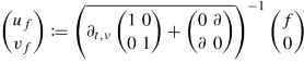
  and

  

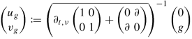
  we have $u_f,u_g \notin \operatorname {dom}(\partial _{t,\nu })$.

Exercise 15.2

Let u and q be defined as in Example 15.1.2. Show that $u\in \operatorname {dom}(\partial _{t,\nu })$ and $q\in \operatorname {dom}(\mathrm {m})$ by explicit computation (not using Theorem 15.2.3).

Hint: Find an ordinary differential equation satisfied by u. Use the explicit solution of this ordinary differential equation to show the claim.

Exercise 15.3

Let $\alpha \geqslant 0$ and ν > 0. Show that

$$\displaystyle \begin{aligned} \partial_{t,\nu} \colon \operatorname{dom}(\partial_{t,\nu}^{\lceil \alpha \rceil+1})\subseteq H_\nu^\alpha(\mathbb{R})&\to H_\nu^\alpha(\mathbb{R}) \\ u\mapsto \partial_{t,\nu}u \end{aligned} $$

is densely defined closable with continuous invertible closure.

Exercise 15.4 (Local Maximal Regularity)

Let H ₀, H ₁ be Hilbert spaces, a ∈ L(H ₁) be such that $\operatorname {Re} a\geqslant c$ for some c > 0. Furthermore, let $C\colon \operatorname {dom}(C)\subseteq H_0 \to H_1$ be densely defined and closed. Let T > 0. Show that for every $f\in L_2\big (\left (0,T\right );H_0\big )$ there exists a unique $u\in H^1\big (\left (0,T\right );H_0\big )\cap L_2\big (\left (0,T\right );\operatorname {dom}(C^*aC)\big )$ with u(0) = 0 such that

$$\displaystyle \begin{aligned} u'(t)+C^*aCu(t)=f(t)\quad (\text{a.e. }t\in \left(0,T\right)). \end{aligned}$$

Hint: Reformulate the equation satisfied by u into an evolutionary equation, apply Theorem 15.2.3.

Exercise 15.5

Let H ₀, H ₁ be Hilbert spaces, a ∈ L(H ₁) be such that $\operatorname {Re} a\geqslant c$ for some c > 0. Furthermore, let $C\colon \operatorname {dom}(C)\subseteq H_0 \to H_1$ be densely defined and closed. Let T > 0. Define $\partial _0 \colon \operatorname {dom}(\partial _0)\subseteq L_2\big (\left (0,T\right );H_0\big )\to L_2\big (\left (0,T\right );H_0\big )$ with ∂ ₀ u = u′ and

$$\displaystyle \begin{aligned} \operatorname{dom}(\partial_0) = \left\{ u\in H^1\big(\left(0,T\right);H_0\big) \,;\, u(0)=0 \right\}. \end{aligned}$$

Show that for $u\in H^1\big (\left (0,T\right );H_0\big )$ the point-evaluation u(0) = 0 is well-defined. Then show that ∂ ₀ + C ^∗ aC is continuously invertible and closed as an operator in $L_2\big (\left (0,T\right );H_0\big )$.

Hint: For the first part use Theorem 12.1.3. For the second part, apply the result of Exercise 15.4. Show that in the situation of the previous exercise, there exists κ > 0 independently of f and u with

$$\displaystyle \begin{aligned} \|u\|{}_{H^1\big(\left(0,T\right);H_0\big)\cap L_2\big(\left(0,T\right);\operatorname{dom}(C^*aC)\big)}\leqslant \kappa \|f\|{}_{L_2\big(\left(0,T\right);H_0\big)}. \end{aligned}$$

Exercise 15.6

Recall Maxwell’s equations from Theorem 6.2.8:

$$\displaystyle \begin{aligned} \partial_{t,\nu}\begin{pmatrix} \varepsilon & 0\\ 0 & \mu \end{pmatrix}+\begin{pmatrix} \sigma & 0\\ 0 & 0 \end{pmatrix}+\begin{pmatrix} 0 & -\operatorname{\mathrm{curl}}\\ \operatorname{\mathrm{curl}}_{0} & 0 \end{pmatrix} \end{aligned}$$

in $L_{2,\nu }\left (\mathbb {R};L_2(\Omega )^{3}\times L_2(\Omega )^{3}\right )$ with $\varepsilon ,\mu ,\sigma \colon \Omega \to \mathbb {R}^{3\times 3}$ satisfying the following property: there exist c > 0 and ν ₀ > 0 such that for all $\nu \geqslant \nu _{0}$ we have

$$\displaystyle \begin{aligned} \nu\varepsilon(x)+\operatorname{Re}\sigma(x)\geqslant c,\quad \mu(x)\geqslant c\quad (x\in \Omega). \end{aligned}$$

By Theorem 6.2.8, for $\nu \geqslant \nu _{0}$ and $j_0\in L_{2,\nu }(\mathbb {R};L_2(\Omega )^3)$, there exists a unique pair $(E,H)\in L_{2,\nu }(\mathbb {R};L_2(\Omega )^6)$ such that

Assume there exist open sets Ω₀, Ω₁ ⊆ Ω such that $\overline {\Omega _0}\subseteq \Omega _1 \subseteq \overline {\Omega _1}\subseteq \Omega$ with $\operatorname {\mathrm {spt}} j_0(t)\subseteq \Omega _0$ for a.e. $t\in \mathbb {R}$. Moreover, $j_0 \in H^{1/2}_\nu \big (\mathbb {R};L_2(\Omega _1)^3\big )$. Furthermore, assume ε = 0 on $\overline {\Omega _1}$. Show that $t\mapsto H(t)|{ }_{\Omega _0} \in H_\nu ^1\big (\mathbb {R};L_2(\Omega _0)^3\big )$.

Exercise 15.7

Let H ₀, H ₁ be Hilbert spaces, a, b ∈ L(H ₁) be such that $\operatorname {Re} b\geqslant c$ for some c > 0. Furthermore, let $C\colon \operatorname {dom}(C)\subseteq H_0 \to H_1$ be densely defined and closed. Let $f\in L_2(\mathbb {R};H_0)$ with $\inf \operatorname {\mathrm {spt}} f>-\infty$. Show that for ν > 0 large enough, there exists for a unique $u\in H_\nu ^2(\mathbb {R};H_0)\cap \operatorname {dom}\big (C^*(a+b\partial _{t,\nu })C\big )$ satisfying

$$\displaystyle \begin{aligned} \partial_{t,\nu}^2 u +C^*(a+b\partial_{t,\nu})Cu=f. \end{aligned}$$

Hint: Use the substitution and to reformulate the equation in question as an evolutionary equation. Then apply Theorem 15.2.3.

References

M. Achache, E.M. Ouhabaz, ‘Lions’ maximal regularity problem with \(H^{\frac {1}{2}}\)-regularity in time. J. Differ. Equ. 266(6), 3654–3678 (2019)
W. Arendt et al., Form Methods for Evolution Equations, and Applications. 18th Internet Seminar, 2015
P. Auscher, M. Egert, On non-autonomous maximal regularity for elliptic operators in divergence form. Arch. Math. (Basel) 107(3), 271–284 (2016)
D. Dier, R. Zacher, Non-autonomous maximal regularity in Hilbert spaces. J. Evol. Equ. 17(3), 883–907 (2017)
G. Dore, L p regularity for abstract differential equations. Funct. Anal. Relat. Top. 1991 1540, 25–38 (1993)
R. Picard, S. Trostorff, M. Waurick, On maximal regularity for a class of evolutionary equations. J. Math. Anal. Appl. 449(2), 1368–1381 (2017)
R. Picard et al., A Primer for a Secret Shortcut to PDEs of Mathematical Physics, vol. 140. Frontiers in Mathematics (Birkhäuser, Basel, 2020)
L. de Simon, Un’applicazione della teoria degli integrali singolari allo studio delle equazioni differenziali lineari astratte del primo ordine. Rend. Sem. Mat. Univ. Padova 34, 205–223 (1964)
S. Trostorff, M. Waurick, Maximal regularity for non-autonomous evolutionary equations. Integr. Equ. Oper. Theory 93(3), Id/No 30, 37 (2021)
Author information
Authors and Affiliations
Rights and permissions
Open Access This chapter is licensed under the terms of the Creative Commons Attribution 4.0 International License (http://creativecommons.org/licenses/by/4.0/), which permits use, sharing, adaptation, distribution and reproduction in any medium or format, as long as you give appropriate credit to the original author(s) and the source, provide a link to the Creative Commons license and indicate if changes were made.
The images or other third party material in this chapter are included in the chapter's Creative Commons license, unless indicated otherwise in a credit line to the material. If material is not included in the chapter's Creative Commons license and your intended use is not permitted by statutory regulation or exceeds the permitted use, you will need to obtain permission directly from the copyright holder.
Copyright information
© 2022 The Author(s)
About this chapter
Cite this chapter
Seifert, C., Trostorff, S., Waurick, M. (2022). Maximal Regularity. In: Evolutionary Equations. Operator Theory: Advances and Applications, vol 287. Birkhäuser, Cham. https://doi.org/10.1007/978-3-030-89397-2_15
Download citation
DOI: https://doi.org/10.1007/978-3-030-89397-2_15
Published:
Publisher Name: Birkhäuser, Cham
Print ISBN: 978-3-030-89396-5
Online ISBN: 978-3-030-89397-2
eBook Packages: Mathematics and StatisticsMathematics and Statistics (R0)