How to Do the Deconstruction of Bioimage Analysis Workflows: A Case Study with SurfCut

Abstract

Published bioimage analysis workflows are designed for a specific biology use case and often hidden in the material and methods section of a biology paper. The art of the bioimage analyst is to find these workflows, deconstruct them and tune them to a new use case by replacing or modifying components of the workflow and/or linking them to other workflows.

This Chapter has been reviewed by Mafalda Sousa, I3S - Advanced Light Microscopy, University of Porto.

FormalPara What You Will Learn in This Chapter

Published bioimage analysis workflows are designed for a specific biology use case and often hidden in the material and methods section of a biology paper. The art of the bioimage analyst is to find these workflows, deconstruct them and tune them to a new use case by replacing or modifying components of the workflow and/or linking them to other workflows.

In this chapter, you will learn how to adapt a published workflow to your needs. More precisely, you will learn how to: deconstruct a bioimage analysis workflow into components; evaluate the fit of each component to your needs; replace one element by another one of your choice; benchmark this new workflow against the original one; and link it to another workflow. Our target for workflow deconstruction is SurfCut, an ImageJ macro for the projection of 3D surface tissue.¹

6.1 Introduction

6.1.1 A Workflow and Its Components

Bioimage analysis workflows and components are defined as follows (Miura and Tosi , 2016): (1) A workflow is a set of components assembled in some specific order to process biological images and estimate some numerical parameters relevant to the biological system under study; (2) Components are implementations of certain image processing and analysis algorithms. Each component alone does not solve a bioimage analysis problem. Components may take forms of a single menu item in image processing software, a plugin, a module, an add-on, or a class in an image processing library. Workflows take image data as input, and output either processed images or numerical values. A workflow can be a combination of components from the same or different software packages and can, for example, come under the form of a script that calls components in a sequence, or a detailed step-by-step instruction on how to chain a sequence of components (Miura and Tosi , 2017; Miura et al. , 2020).

6.1.2 What Is Deconstruction?

Bioimage Analysis Workflows are designed for specific purpose, so usually, they cannot be used as a general tool for different problems. Then how can we learn how to create bioimage analysis workflows? One way is to do everything from scratch. Another way is to learn from other bioimage analysis workflows, modify them, and reassemble components to create something new for a specific purpose. We call this (a workflow) "deconstruction". The process of deconstruction was initially proposed by Jacques Derrida, a French philosopher, as a criticism against the modern philosophy. Instead of constructing ideas, which implicitly builds on hidden but solid principles as the base of such construction, deconstruction is a way of shifting ideas by critical thinking, sometimes denial, and in other times the restructuring of preexisting principles.

The deconstruction of bioimage analysis workflow was introduced as a pedagogic method for the Bioimage Analyst School of NEUBIAS. Deconstructing a workflow means identifying and isolating each of its components in order to assess their quality and possibly replace them with more suitable components. In addition to using it as a powerful pedagogical tool, one of the main interest in deconstructing a workflow is to avoid spending time and effort "re-inventing the wheel", and instead to re-use, optimize or adapt an existing method to the new users’ needs.

6.1.3 A Case of Study of Workflow Deconstruction: SurfCut

The ImageJ macro "SurfCut" was chosen as a study case for workflow deconstruction during the NEUBIAS training school TS15 (Bordeaux, March 2020). Interestingly, this led to numerous new ideas and ways to implement SurfCut. Some trainees added GPU processing capability with CLIJ (Haase et al. , 2020), while others completely re-wrote the workflow in Python² and Matlab³ and benchmarked the different versions (SurfCut, GPU-SurfCut, Python-SurfCut and Matlab-SurfCut). Furthermore, this deconstruction session, along with the writing of this book chapter, also prompted us to develop a new version of the SurfCut macro, SurfCut2, including a complete refactoring of the code (as described in this book chapter), bug-fixing, and addition of new functions.⁴ In this chapter, we explain in detail the procedure for workflow deconstruction based on these experiences, using SurfCut as an example target workflow.

6.1.4 What Is SurfCut?

SurfCut is an ImageJ macro that allows the numerical extraction of a thin, curved, layer of signal in a 3D confocal stack by taking as reference the surface of a 3D biological object present in the volume of the stack (Erguvan et al. , 2019). The macro is written in the ImageJ1.x(IJ1) macro language, and runs on the Fiji platform (Schindelin et al. , 2012). Using built-in ImageJ functions, the biological object in the image is blurred, segmented, filled, shifted in the Z-axis at two different depths and used as a mask to erase unwanted raw signals at a chosen distance from the surface of the detected object (Fig. 6.1, and detailed description in Sect. 6.4). The whole workflow can be viewed as a sort of “object surface”-guided signal filtering method. This allows the removal of unwanted signals relative to the surface of the biological object and the extraction of specific structures from the 3D stack, such as the cell contours (Fig. 6.1) or outer epidermal cortical microtubules. As such, this workflow has already been incorporated as a component of larger workflows, as a preprocessing step for cell segmentation or cortical microtubule signal quantification (Erguvan et al. , 2019; Takatani et al. , 2020; Baral et al. , 2021).

Fig. 6.1

Overview of SurfCut principle and output, applied on Arabidopsis thaliana cotyledon epidermal cells stained with propidium iodide and imaged in 3D with a confocal microscope. Top panel is a combination of half of the raw confocal signal (grey) and half of the "SurfCut-extracted" signal (red), partially overlapped and tilted in 3D to show the relationship between the raw signal and output. Bottom left panel is a max-intensity projection of the raw signal. Bottom right panel is a max-intensity projection of the "SurfCut-extracted" signal, highlighting how the process efficiently preserves the cell contour (anticlinal) signal in the epidermal layer while removing signal from the periclinal cell contours

6.1.5 What Was SurfCut Developed for?

SurfCut was originally developed as a pre-processing tool to filter out unwanted signals and perform a Z-projection prior to 2D segmentation of epidermal plant cells. The so-called “puzzle-shaped pavement cells” of the leaf epidermis harbor very particular shapes (Fig. 6.1). This is a very interesting system to study the morphogenesis of single cells in a tissue context. To understand how these cell shapes emerge, a proper shape quantification with several genetic backgrounds, or under specific treatment conditions, is required. Many methods were developed to quantify and compare cell shapes based on 2D cell contours (Möller et al. , 2017; Sánchez-Corrales et al. , 2018; Wu et al. , 2016). As the leaf epidermis is a 3D curved surface, a Z projection is required prior to the use of any of these tools. Given the lack of available user-friendly tools to perform a proper extraction of 2D cell contours from 3D confocal stacks, we developed SurfCut (Erguvan et al. , 2019).

Although the SurfCut macro was written in the context of a biological project and could have ended (somewhat hidden) in the "Material and method"—section of a larger biological publication (still in preparation at the time of writing this chapter), we decided to publish it separately (Erguvan et al. , 2019), to assign a DOI to the code and provide image data, also identified with a DOI (Erguvan and Verger , 2019), to enable testing of the macro. We think that the publishing of this type of macro gives more visibility to the bioimage analysis workflows and, by giving all the space needed to the description of the workflow, ensures a greater reproducibility.

6.1.6 Other Similar Tools

Before developing SurfCut, we had identified in our bibliographical searches other workflows performing apparently similar outputs, but none of them fitted exactly our needs. As described in Erguvan et al. (2019), we were originally using the software MorphoGraphX (MGX) (Barbier de Reuille et al. , 2015) that provides a very accurate solution to our problem (Erguvan et al. , 2019; Verger et al. , 2018), but requires too many manual steps and does not easily allow batch processing. In addition, Merryproj (Barbier de Reuille et al. , 2005), SurfaceProject (Band et al. , 2014), LSM-W2 (Zubairova et al. , 2019) and Smooth 2D manifold (Shihavuddin et al. , 2017) were discussed in Erguvan et al. (2019) and were found inadequate for our purpose. After the independent publication of the SurfCut macro, we discovered other workflows that our first search had not revealed, such as the ImageJ macro identifyuppersurfacev2 (Galea et al. , 2018),⁵ or the ImageJ plugin MinCostZSurface (Li et al. , 2006).⁶ We also identified more advanced workflows that would not have fitted our needs w.r.t. simplicity (Schmid et al. , 2013; Heemskerk and Streichan , 2015; Candeo et al. , 2016). Furthermore, since the publication of SurfCut, additional workflows, such as the ImageJ plugins Ellipsoid Surface Projection (Viktorinová et al. , 2019) and SheetMeshProjection⁷ (Wada and Hayashi , 2020) were developed to serve a similar purpose. In total, there are at least ten different workflows that can perform the type of signal layer extraction that SurfCut performs. While all these tools allow the generation of relatively similar output, almost all of them use a different approach. In addition, they are tailored to specific needs, such that some of these tools outperform others on a certain type of images, thus offering a large choice of alternative workflow components to perform this specific pre-processing step.

In the following sections, we present how to deconstruct SurfCut Erguvan et al. (2019), i.e. how to identify its different components in the reference publication and in the code. We then explain how to refactor the code, replace one component and benchmark the new workflow against the original one. Finally, we explore how to integrate this workflow with other workflows.

6.2 Dataset

The SurfCut macro was released with test image data of around 535 Mb. This data set was uploaded to Zenodo with a thorough description of the imaging conditions, and identified with its DOI: http://doi.org/10.5281/zenodo.2577053 (Erguvan and Verger , 2019).

6.3 Tools

• Fiji: Download and install Fiji on your computer   (https://imagej.net/Fiji/Downloads)

• ImageJ macro SurfCut: Download the "SurfCut.ijm" macro file to your computer (https://github.com/sverger/SurfCut). To run the macro in Fiji either click on Plugins>Macro>Run and select "SurfCut.ijm", or drag and drop "SurfCut.ijm" into the Fiji window and click run.

• ImageJ macro SurfCut2: Download the "SurfCut2.ijm" macro file to your computer (https://github.com/VergerLab/SurfCut2). Follow the same instructions as for the ImageJ macro SurfCut.

• ImageJ macro used for exercises in this chapter can be found at: https://github.com/NEUBIAS/neubias-springer-book-2021

6.4 Workflow

In this section, we propose a step-by-step deconstruction and modification of the SurfCut workflow. The concepts and exercises in each step can be generalised to any kind of bioimage analysis workflow.

We take the following steps for the deconstruction of the workflow:

• Step 1: Identify components in the description of a workflow and in the code;

• Step 2: Draw a workflow scheme;

• Step 3: Identify limitations on input format, processing capabilities, simplicity to re-use;

• Step 4: Identify block of codes corresponding to components;

• Step 5: Refactor code;

• Step 6: Replace a component of the workflow;

• Step 7: Compare the performance of the original workflow with a modified one;

• Step 8: Link this workflow with another workflow.

6.4.1 Step 1. Identification of Components in the Textual Description

When working with a published workflow, the first step is to identify the components in the text of the publication and the order in which they are used. Nowadays, published workflows are often accompanied by a detailed user manual and/or a "readme" if the code is released on GitHub or GitLab. This text can also contain additional information on the components and on the links between them.

Exercise 1

• 1. Read Erguvan et al. (2019) and underline in the text all elements describing the components of the SurfCut workflow. Then summarize the result as an ordered list of components.

• 2. Which additional useful information relative to the components can you find on the GitHub repository of the SurfCut macro⁸?

Solution to Exercise 1

• 1. All text elements describing the components of the SurfCut macro in Erguvan et al. (2019) are on page 3 in the Methods section, in the "2D cell contour extraction with SurfCut" paragraph:

  • "The macro has two modes: (1) “Calibrate,” [...], and (2) “Batch,” [...]".

  • "The stack is first converted to 8 bit."

  • "De-noising of the raw signal is then performed using the Gaussian Blur function."

  • "The signal is then binarized using the Threshold function."

  • "an equivalent of the “edge detect” process from MGX⁹ is performed [...]; each slice from the binarized stack, starting from the top slice, is successively projected (Z-project) [...]. This ultimately creates a new binary stack in which all the binary signals detected in the upper slices appear projected down on the lower slices, effectively filling the holes in the binary object."

  • "This new stack is then used as a mask shifted in the Z direction, to subtract the signal from the original stack above and below the chosen values depending on the desired depth of signal extraction."

  • "The cropped¹⁰ stack is finally projected along the Z-axis using the maximal fluorescence intensity in order to obtain a 2D image."

  The SurfCut workflow has 6 components: (1) bit-depth conversion, (2) denoising, (3) thresholding and binarization, (4) edge detection, (5) masking, and (6) Z-projection. The workflow can be run one component at a time, to allow for selection of parameters per component (calibrate mode), or automatically (batch mode) (Fig. 6.2).

• 2. In the GitHub repository of the SurfCut macro, a careful reading of the "readme" and user guide¹¹ identifies and confirms the components found in the text of the publication. Note that dialog boxes to interact with the user are not considered as components of the workflow.

Fig. 6.2

Output of each processing step of the SurfCut workflow

6.4.2 Step 2. Drawing a Workflow Scheme

We identified above the workflow components from the text. Let us now draw a scheme of the workflow. A workflow scheme summarizes and links all the components of a workflow. This scheme will serve as a guide to get an overview of the workflow, and identify those components in the code that can be refined after Step 4, if needed. Figure 6.3 is a graphical scheme of a general bioimage analysis workflow.

Fig. 6.3

Workflow scheme example

Exercise 2

Utilizing information found in Exercise 1, draw the scheme of the SurfCut workflow: start drawing one box per component following the guidelines in Step 1. Then identify each component by a short informative name and link components with each other, so that the input of a component is an output of the previous component.

Solution to Exercise 2

The SurfCut macro has two modes: (1) "calibrate", where the components are executed one-by-one and only once, and (2) "batch", where the complete workflow is repeated on several images. We draw a batch component to illustrate the batch mode. We then draw the 6 components of the workflow inside the batch component and link them in the order in which they appear in the text: Component 1 performs the conversion to 8-bit pixel representation, Component 2 performs the denoising, etc. In the text, we will now refer to components using the following wording: Component 1 "8 bits conversion", Component 2 "Denoising", etc.

For simplicity of the scheme, we ignored import and export components (such as User-Interface for file selection or saving of results). These can be included as well, especially if the import or export components correspond to non-trivial steps (e.g. specific data format).

6.4.3 Step 3. Assessment of Prerequisites and Limitations

In the two previous steps, we identified the components of the workflow described in the publication and drew a workflow scheme. We now have an overview of the workflow and can make more confident assessment on if the workflow is appropriate to solve our biological question or not. To determine if we can use the workflow as it is, if it is sufficient to only change a couple of the components to adapt the workflow to our data, or if the workflow is not adequate at all for our data, we need to make some additional (final) checks:

• Data format compatibility: Is the input format (.tif, .png, .czi...) and type of data (2D, 3D, time-series) that we have compatible with the format and type required by the workflow?

• Processing capacity: Is the amount and size of the data compatible with the workflow (fully manual workflow or very slow workflow versus high content screening data; included calibration step requiring a minimum of 30 images versus 5 images available only...)?

• Data content compatibility: Are the type of biological data and markers that we have to work with compatible with what is considered in the workflow (membrane marker versus nuclear marker, epithelial marker versus whole tissue marker, flat versus curved tissue...)?

• Output adequacy: Will the output data generated by the workflow (new images, numerical values, plots...) be actually useful for what we intend to do (get biological results, benchmark the workflow against another, embed in a larger workflow...)?

If the answer is no to one, or several of these questions, the next question to answer is: Could one, or several of the components be replaced by a more adapted or efficient one(s)? Here we assume that the macro language and the use of ImageJ/Fiji is not an obstacle for any bioimage analyst. For other more advanced or less known languages, as well as more exotic software, another sequence of preliminary checks would be:

• Language: In which language is this workflow written?

• Platform: On which platform can I execute it?

• Inter-operability: How complex will it be to link this workflow to my other tools written in another language or executed on another platform?

• Code migration capability: In case I need to make some modifications to the workflow, do I have other options than fully rewriting it in my favorite language?

Exercise 3

• 1. Install the SurfCut macro and execute it on the associated data.

• 2. Identify, based on the text of the reference publication, the "readme" in the Github repository and the user guide, all elements restricting the datasets of certain type to be used with SurfCut.

• 3. For each use case below, download the dataset and explain if and why the dataset could be processed directly with SurfCut, without any workflow modification, using the checks defined above. We assume that the output of the workflow (a 2D projection) is what we need.

  • (a) Use case 1: 3D light sheet microscopy images of a Tribolium epithelium (Vorkel et al. , 2020).

    Dataset: https://zenodo.org/record/3981193#.Xzo8pTU6-60, take "Strausberg_Tribolium_LAGFP_tailpole_runC0opticsprefused301310.tif". This dataset was used as an example to showcase another projection tool.¹²

  • (b) Use case 2: 3D confocal and spinning disk microscopy images of Drosophila epithelia (notum and wing disc, Valon and Staneva , 2020).

    Dataset: https://zenodo.org/record/4114074#.X5AJAe06-60. Take the image named "notum2_GFP.tif".

  • (c) Use case 3: 3D light sheet microscopy images of single cells (Driscoll et al. , 2019).

    Dataset: https://cloud.biohpc.swmed.edu/index.php/s/Z9j62 w2FCareyJY/download), in the folder called "testData". Each image is associated with a text file describing the imaging conditions (AcqInfo.txt). There are three examples of MV3 melanoma cells ("krasMV3") and one example of conditionally immortalized hematopoietic precursors to dendritic cells ("lamDendritic"). Associated GitHub repository: https://github.com/DanuserLab/u-shape3D and research article: https://www.ncbi.nlm.nih.gov/pmc/articles/PMC7238333/.

  • (d) Use case 4: light sheet image of a gastric cancer spheroid (Rocha et al. , 2020).

    Dataset: https://zenodo.org/record/4244952#.X6L_ZIj7SHs.

Solution to Exercise 3

• 1. See Sects. 6.2 and 6.3, as well as the installation instructions and the userguide on the GitHub repository.¹³

• 2. Prerequisites

  Pre-requisites and limitations found in the main text of the publication:

  • "the acquired signal must be strong and continuous enough at the edge of the sample in order for the signal to be detected and segmented from the background noise by a simple conversion to a binary image." (Methods section, in "Confocal microscopy")

  • "avoid the presence of artifacts, e.g., from stained cell debris or bacteria at the surface of the sample." (Methods section, in "Confocal microscopy")

  • "The first slice of the stack should be the top surface of the sample in order for the process to work properly." (Methods section, in "2D cell contour extraction with SurfCut")

  • "a new method (SurfCut) to extract cell contours or specific thin layers of a signal at a distance from the surface of samples in 3D confocal stacks." (Results and discussion section, "2D cell contour extraction from 3D samples with MGX¹⁴ and SurfCut")

  • "the associated error can become important for samples with high curvature." (Results and discussion section, "2D cell contour extraction from 3D samples with MGX and SurfCut")

  • "In principle, this tool may be used on any 3D stack (e.g., confocal or light-sheet microscopy) originating from either animal, fungi, or plant systems." (Conclusions section)

  • "SurfCut is particularly well suited for tissues with a low curvature " (Conclusions section)

  • "SurfCut is very well suited for high-throughput pavement cell contour extraction and further quantification. [...] Besides, SurfCut can also be used to extract other types of signals, such as cortical microtubules, allowing a suppression of the background noise coming from the signal below." (Conclusions section)

  • "SurfCut can be a very useful tool for the 2D representation (from image-based screening protocols to publication figures) of 3D confocal data in which overlapping signal from different depths in the stack hinders the visualization of signal or structures of interest." (Conclusions section)

  Prerequisites and limitations found in the "readme" of the GitHub repository:¹⁵

  • "This can, for example, be used to extract the cell contours of the epidermal layer of cells." (Description section)

  • "SurfCut [...] is in principle only adequate for sample with a relatively simple geometry." (How it works section)

  • "3D confocal stacks in .tif format, in which the top of the stack should also be the top of the sample." (Prerequisites section)

  Prerequisites and limitations found in the user guide:¹⁶

  • "Our image analysis pipeline was developed to extract cell contours or specific layers of signal in confocal images of plant samples, but can in principle be used on any 3D fluorescence microscopy stack (e.g. confocal or light-sheet microscopy) originating from either animal, fungi or plant systems, stained or expressing a fluorescent reporter highlighting the cell contours (typically, a protein at the plasma membrane). For a better-quality output, it is recommended to use a Z interval of maximum 1 $\mu$m." (Procedure section, A. Image Acquisition)

  • "if your signal is very heterogeneous, e.g. for cortical microtubules, a higher [Gaussian blur radius] value can help homogenize the signal and obtain a good surface detection." (Procedure section, C. Calibration, step 6.)

  • "The voxel properties of your image in micrometers, are automatically filled based on the metadata of the image. If no data is found, these values will all be set to 1." (Procedure section, C. Calibration, step 10.)

  • "Remember that the stack should be in .tif and that the top of the stack should also be the top of the sample." (Procedure section, D. Running the script in batch mode, step 18.)

• 3. Use cases

  • Use case 1: 3D light sheet microscopy images of a Tribolium epithelium.

    We have a 3D stack, .tif format, we know the pixel size, and the life-actin GFP marker signal delimits well a relatively thin epidermal layer. However, these are time-lapse data (SurfCut can process only one time-point at a time), and the tissue is very curvy. The data could be processed by first extracting each individual time points and then analysing the images in a batch after having defined the proper parameters in the calibrate mode. However, SurfCut is not recommended in this case due to the high curvature of the tissue.

  • Use case 2: 3D confocal and spinning disk microscopy images of Drosophila epithelia (notum and wing disc), image named "notum2_GFP.tif"

    We have a 3D stack, in .tif format. We know the pixel size from the description of the Zenodo upload, and the E-Cadherin marker delimits well a relatively thin epidermal layer, which is only slightly curved. SurfCut is appropriate here, since the tissue is not too curvy. Moreover, SurfCut can help remove noise above and below the epidermis and hence render a sharper projection of the cell contours. After adding the pixel size specified in the description of the dataset to the metadata of the image, we can process the image with SurfCut using the following parameters: gaussian blur of radius 3; threshold of 50; top = 6; bottom = 11.

  • Use case 3: 3D light sheet microscopy images of single cells.

    We have 3D stacks, .tif format, and we know the pixel size from the AcqInfo.txt file. However, these are 3D closed objects with quite some relief. Here SurfCut is not appropriate to project the 3D stacks, it would deform the cells too much.

  • Use case 4: 3D light sheet images of a gastric cancer spheroid.

    We have a 3D stack in .tif format. However, the stack contains the first bright and blurry slice that needs to be removed first, the proper voxel size needs to be set based on the information found in the description of the dataset, and the z resolution is rather low (5 micron) compared to the x and y (1 micron). SurfCut can help remove noise around the spheroid, as well as the blur from inside, and render a sharper projection of the surface. We can process the stack with SurfCut using the following parameters: Gaussian blur of radius 3; threshold of 20; top = 0; and bottom = 25.

6.4.4 Step 4. Identification of Components in the Code

In the previous steps, we identified the components of the workflow from the text, drew a workflow scheme (see Fig. 6.4) and checked the prerequisites in terms of data input. If the workflow could be reused as it is, we could have stopped there. Now, we assume that we need to modify the workflow to adapt it to our needs. Hence we need to get a more in-depth knowledge of the code.

Fig. 6.4

SurfCut workflow scheme

Each programming language has a different syntax, but there should always be comments, variables with meaningful names, functions, and other common recognizable items. They can help you understand the structure of the workflow in the code. Read first the comments around the code to identify the different components of the workflow, as found in step 1 and 2 (see Fig. 6.4). Each component should ideally match with a block of code containing one or several built-in or custom functions, some loops and conditional statements etc. To further understand the order of execution of the workflow, identify also the different input and output variables.

SurfCut contains several defects often found in real codes, and especially in ImageJ macros.¹⁷ We will see, for instance, in the exercise below that, in SurfCut, some components are spread over several blocks of code and intermingled with other components. We will see also that some components in SurfCut are made of several built-in functions that are not wrapped in one bigger function. Of course, a modular code with clearly separated blocks of code and one function per component is easier to read and understand, but SurfCut is a representative of ImageJ macros. This lack of structure comes from two elements: (i) macro authors are seldom software developers and hence lack good code writing practices (commenting, wrapping components into functions...) and (ii) most macro authors rely on the macro recorder to find the proper functions to use. The macro recorder prints the macro commands corresponding to the steps done manually by the user through the graphical user interface of ImageJ/Fiji. Whereas some components corresponds to a single ImageJ macro built-in function (e.g. a Gaussian blur), other require several functions (e.g. Edge detect). The modular structure with components is lost when using the macro recorder. In addition to these defects, SurfCut contains many repetitions of code lines. This is due to the presence of two types of workflows in one code, the calibrate and the batch workflows, and the lack of optimization in the code to reuse functionalities of one workflow in the other rather than copy functionalities.

As explained in the introduction, we took into account all these defects and carried out a complete refactoring of the code (as described in Step 5 and 6 of this book chapter), fixed bugs, and created new functions to reach a new version of SurfCut, called SurfCut2.¹⁸ We also made a simpler version of the macro, called SurfCut2-Lite. We propose two alternatives to the exercises below, corresponding to two levels of difficulty. For the beginner level, use the SurfCut2-Lite code¹⁹ and do the exercises 4.1, 6, 7 and 8 (skip exercise 4.2 and 5, which are already implemented in the code of SurfCut2-Lite). For the advanced level, use the code of the original SurfCut macro and follow all the steps and exercises proposed.

Exercise 4

Using either SurfCut2-Lite code ("beginner level") or SurfCut code ("advanced level"):

• 1. Identify blocks of code corresponding to the different components identified in Step 1 and Step 2.

• 2. Extract in a separate text file a minimal version of the macro corresponding to the workflow only: remove user interfaces, "for" loops used to run the batch mode, and "while" loops (in this case, they are not a part of the workflow). Keep only the essential elements the workflow and group elements corresponding to a given component together. Identify the different components of the workflow using the comments present in the macro.

Solution to Exercise 4

"Beginner Level": Response to Task 1, Considering SurfCut2-Lite Code

• 1. The workflow appears once, and can be identified at the early part of the macro, in the form of a suite of user-defined functions (line 51–68; similar to the solution of Exercise 5.2). Further, all the components of the workflow are organized as user-defined functions, between line 112 and 222 of the macro (Component 1: line 114–118; Component 2: 120–124; Component 3: 126–131, Component 4: 133–156; Ccomponent 5: 158–207; Component 6: 209–215; similar to exercise 5.1 solution). Note that the Component 5 was split into two user-defined functions (ZAxisShifting and masking), which can be useful and will be explained later in this book chapter.

"Advanced Level": Response to Tasks 1 and 2, Considering the Original SurfCut Code

• 1. In the original SurfCut code, the workflow is present twice: Once in the "Calibrate" mode, in which most of the steps are intertwined with user input and interaction, and once in the "Batch" mode, in which the backbone of the macro is embedded in a batch processing "for" loop. The most easily identifiable backbone of the workflow is present between lines 403 and 463 of the macro (Component 1: line 403; Component 2: 404; Component 3: 407–409, Component 4: 418–431; Component 5: 433–453; Component 6: 462–463), within the "Batch" mode part of the code. In the "Calibrate" part of the code, equivalent code blocks can be found at lines 68–88 and 161–200.

• 2. The code below shows a possible solution for the extraction of the minimally required code for the core functionalities of SurfCut. Each component is labeled in a corresponding comment by its corresponding number (see Fig. 6.4).

  

  Code available in the GitHub repository of this book.²⁰

6.4.5 Step 5. Code Refactoring

In Step 4, we identified the basic components of the workflow in the code and extracted a minimal version of the code. To simplify the later replacement of a component in the code, we propose an optional step: refactoring the code. This step aims at reorganizing the code in order to improve its design and re-usability without changing its input or behavior. The refactored code will be constituted of several user-defined functions, each corresponding to one component of the workflow. The replacement of a component is then equivalent to replacing a function.

Here, we also suggest to split one of the components into two, as a part of the refactoring process. Indeed, while some of the workflow components described in the publication text (and identified in Step 1 and Step 2) correspond to single ImageJ built-in functions, Component 4, "Edge detection", and Component 5, "Masking", with implementation inspired by the algorithm used in the software MorphoGraphX, correspond to many lines of code directly coming from the macro recorder. To improve the organization and re-usability of the code, here we suggest splitting the code corresponding to Component 5, "Masking", in two components. The purpose of Component 5 is to extract a layer of signal in the original stack, using the mask created in the preceding "edge-detection" step. This works by successively shifting the mask down and subtracting the signal twice: once above and once below the signal of interest. So, in fact, it is not only a masking step, but also a Z-axis shifting of the mask preceding the masking. Here, we propose to keep roughly the same process, but reorganize the order in which the steps are taken and separate these two steps: to first create a layer mask by two successive Z-axis shifts of the original mask and subtraction from one-another (Component 5a), and then to do the masking itself (Component 5b).

Overall, such a substantial re-refactoring costs some time and brainpower, but can strongly improve the workflow and ultimately simplify the replacement of components or their parts, as we will see in the next step.

Exercise 5 ("Advanced Level" Only, Using the Original SurfCut Code)

• 1. Inspect each component extracted in Step 4, identify unnecessary or disorganized lines of code and optimize the code of each component by simplifying, cutting, and reorganising the code lines.

  Convert each component into a user-defined function.²¹

  As discussed above, re-implement Component 5 of the workflow into two steps: (5a) Layer mask creation, and (5b) Raw signal masking.

• 2. Write, or extract from the original SurfCut macro, the lines corresponding to the definition of the input and the parameters necessary to run the code.

  Make a working macro including the definition of parameters at the beginning and the fully refactored version of the workflow (optimized code, user-defined functions, and with Component 5 split in two parts).

Solution to Exercise 5

• 1. A possible refactoring of the initial code into functions, with the re-implementation of Component 5 in two parts, is shown below. Some of the variable names have been homogenized, some unnecessary code lines (e.g. wait(1000);) have been removed, and all the components have been transformed into simple user-defined functions. To get a better insight, compare the code proposed below with the equivalent code extracted from the SurfCut macro in Step 4.

  

  

  

  Code available in the GitHub repository of this book.²²

• 2. The code for opening an image and getting the variable names can be found in lines 32–38 of the original SurfCut macro. Variables related to the radius of the Gaussian blur filter, threshold for the segmentation, and top and bottom depths (in micron) for masking can be found in lines 42–45 and 149–150. These variables are used for the definition of Cut1 and Cut2 (the actual values of the Z-axis shifts, depending on the thickness of the stack slice steps). The values of Cut1 and Cut2 depend on the stack slice thickness, which, in the macro, is extracted from the metadata of the image (line 96). For simplicity, we can here define it directly in the code.

  In the solution below, the parameters identified above are called at the beginning of the macro. The functions defined in the answer to Question 1 (above) are successively called, giving a clear overview and easy reading of the workflow.

  

  Code available in the GitHub repository of this book.²³

6.4.6 Step 6. Replacing a Component: Shift Mask in the Z-Axis Direction

Now we have a well organized and flexible workflow. It is time to inspect it in detail and determine if the different components are best adapted to our needs. As an example, we will now examine the Component 5a "Layer mask creation" created during the refactoring of the SurfCut macro code (line 76–107); this component is included in the SurfCut2-Lite code (line 158–197). In the current implementation, we use a sequential Z-axis shift of the mask to make a layer-mask. But in principle, as discussed in (Erguvan et al. , 2019), a 3D erosion, although more computationally demanding, would be more suitable for samples with high curvature. Let us try to replace the Component 5a with a procedure which uses a 3D erosion instead of a Z-axis shift.

Exercise 6

• 1. Find how to perform a 3D erosion on a binary object using Fiji.

• 2. Write a function similar to the existing Component 5a, but performing a 3D erosion on the mask, instead of Z-axis shift ( to be used to replace Component 5a).

• 3. Modify the refactored version of SurfCut or SurfCut2-Lite to include both alternatives for processing (Z-axis shift and erosion) with a conditional statement.

Solution to Exercise 6

• 1. 3D erosion operation is available in Fiji Plugins>Process>Erode(3D). The macro recorder can be used to record the corresponding code. Alternatively, we can apply the erosion operation from the 3D suite plugin (Ollion et al. , 2013).²⁴

• 2. Below we propose a user-defined function that takes as input parameter two "erosion depths", i.e. two distances (in pixels or microns) form the surface, defining the upper and lower boundary of the signal to be extracted. This function processes the binary stack ("Mask") obtained with the EdgeDetect. The mask is eroded by several erosion steps using a "for" loop. The number of steps depends on the value of the first erosion depth. The image resulting from this first erosion is then duplicated and eroded further to reach the second defined value of erosion depth. The first eroded stack is then inverted (in terms of binary values), and these two eroded stacks (binary values) are summed, forming a layer mask ("LayerMask") that can then be used in Component 5b.

  

  Code available in the GitHub repository of this book.²⁵

• 3. In the example below, we added the new component 5a as a function. We either call the Z-shift or erode function, using a conditional "if" and "else if" statement (lines 27–31 below). In addition, we defined new variables necessary for the new erode function and for the conditional statement (lines 9–11): Ero1 and Ero2 which are calculated from the values Cut1 and Cut2, and MODE, in which the user can define whether to process the macro with the Z-axis shift, or using the erosion.

  

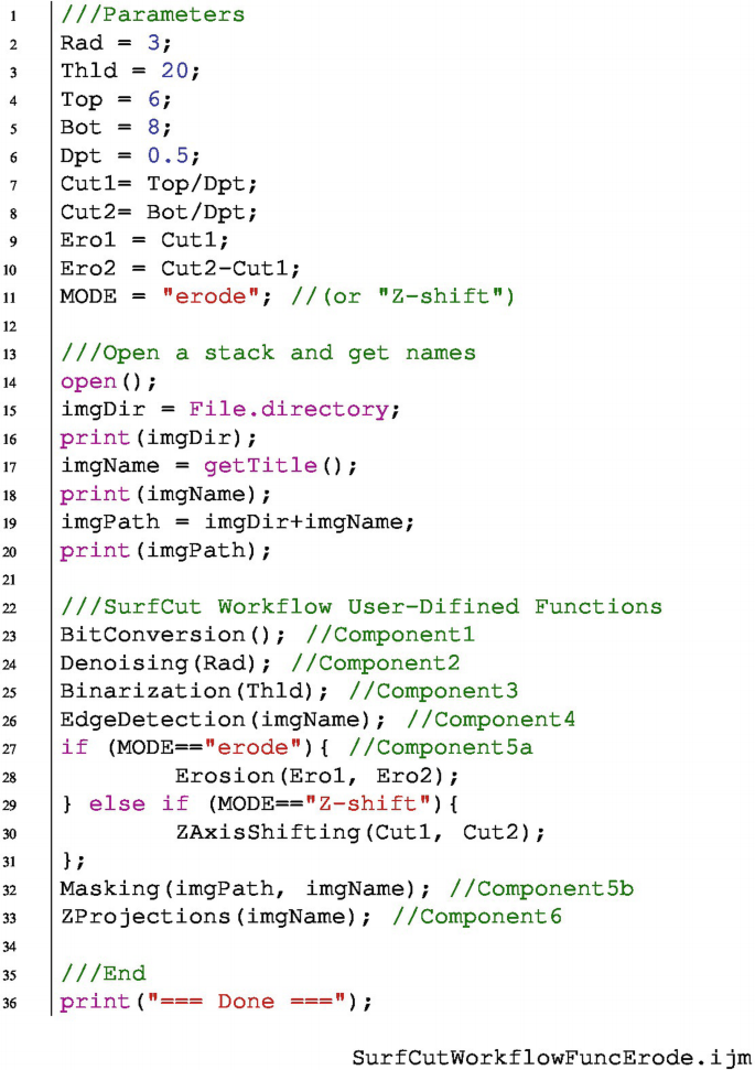
  Code available in the GitHub repository of this book.²⁶

6.4.7 Step 7. Benchmarking: Comparison of Two Alternative Components

Benchmarking is assessment of benefits and drawbacks of different algorithms and evaluation of their performance in terms of a range of criteria: speed, memory usage when dealing with, e.g., 2D or 3D stacks, and quality of the result (e.g., How much the projection deforms the image? How well does the selected filter extract the features of interest in the image?). Benchmarking can be performed for two (or more) similar components, or two (or more) similar workflows. Here, we would like to assess if the change of a component that we made in Step 6 is beneficial for the workflow.

In Step 6, we suggested an alternative code for layer mask creation. We will now benchmark this new workflow against the original one. First, we can look at the output and qualitatively assess if the workflow generates the expected result. Second, and important—we will quantitatively assess the impact of the change on the performances of the workflow, mainly evaluating if the processing time is a limiting factor. This can be done very quickly by adding timestamps in the script, and calculating the time elapsed between the beginning and the end of the workflow execution. Furthermore, using nested "for" loops, it is also possible to iteratively test how different parameters affect the workflow processing time: Erode or Z-shift, and increasing depth of masking. The values can also be recorded in a text file to make a direct comparison of the performance after running the benchmark.

Exercise 7

• 1. Find out how to add a timestamp in the macro.

• 2. Implement a way to quantify the processing time of the macro.

• 3. Implement a way to record the processing times in a text file.

• 4. Implement nested "for" loops to iteratively test the Erode and the Z-shift, as well as the increasing depth of masking, starting from 1 (Top) and 2 (Bot), and reaching 5 (Top) and 6 (Bot) (1–2, 2–3, 3–4, 4–5, 5–6). Furthermore, a simple way to decrease processing time in ImageJ macros is to use the "setBatchMode" function. It allows the processing of the images to be carried out without displaying the images, which can improve processing time by up to a factor of 20. Implement an additional nested loop to test how much the "setBatchMode" function improves the performances of the macro.

• 5. Run this modified version of SurfCut on the provided SurfCut data (see Section 6.2) and compare the performances of the two components.

Solution to Exercise 7

• 1. Within the ImageJ built-in functions, there are at least two ways to add a time-stamp: "GetDateAndTime" and "GetTime". The latter is more practical to calculate the elapsed time, because it gives a value in milliseconds, instead of hours:minutes:seconds:milliseconds (which is less practical for further analysis).

• 2. "GetTime" can be added right before and right after the execution of the workflow of interest. Subtracting the value given at the first time point from the value obtained at the second time point gives the elapsed time.

  

• 3. A text file can be created with the built-in function "File.open", it can be closed using the function "File.close", and text can be added to the closed file with the function File.append. Note that, while the text can also be written directly in an open text file with the "print" function, only one file can be opened at a time, which can be limiting in some situations (e.g. if other parameters are being recorded by the macro in another text file).

  

• 4. Three nested "for" loops need to be implemented to iteratively test the three types of parameters of interest. This requires to slightly reorganise where the variables are defined, since a number of them are now defined in the "for" loops. A text file is saved containing the output of all the time elapse measurements along with the parameter used at each iteration. The SurfCut 2D projection is also saved in each case, in order to assess the quality of the output. A possible complete solution is shown below.

  

  

  

  Code available in the GitHub repository of this book.²⁷

• 5. With the Erode component, the processing time increases linearly with the number of erosion steps required. This is not the case with the Z-axis shift component. However, the accuracy and quality of the result for samples with higher curvature are in principle improved with the Erode process, as described in (Erguvan et al. , 2019).

6.4.8 Step 8. Linking to Another Workflow: FibrilTool

As described in the introduction and the reference publication, SurfCut was designed, and has been used, as a pre-processing step for cell segmentation and cortical microtubule (CMT) signal analysis with another ImageJ macro called FibrilTool (Boudaoud et al. , 2014). In this case, SurfCut and FibrilTool are two components of a workflow. However, the output of SurfCut cannot be directly taken as the input of FibrilTool. As a final exercise, we will analyse how these two components can be linked in a workflow, by adding one, or several, intermediate components.

Exercise 8

• 1. Identify the type of input required for the FibrilTool macro.

• 2. Identify the missing steps between the SurfCut output and the FibrilTool input, required to connect the two components.

• 3. How would you implement these missing steps?

• 4. Last but not least, consider whether the required tools already exist, or you need to implement them de novo.

Solution to Exercise 8

• 1. FibrilTool takes as input an ImageJ ROI and a corresponding image containing the fibrilar structure to analyse (e.g. CMTs).

• 2. Surfcut can directly generate one of the FibriTool inputs: the preprocessed CMT image. It can also generate the cell contour image. The missing step here is the generation of ROIs from this cell contour image. Finally, the originally published version of FibrilTool takes and analyses ROIs manually one by one. Since many ROIs per image can be created, FibrilTool could be automatized to analyse all these ROIs automatically, one after the other.

• 3. For generation of ROIs from a cell contour image, a simple Analyze particle function may be sufficient. However, to ensure better results, a watershed segmentation could be used. For FibrilTool automation, a "for" loop can be implemented to analyse automatically all ROIs generated in the preceding step.

• 4. The second part of the user guide of SurfCut describes these additional workflow components. Previously, an automated version of Fibriltool that uses ROIset.zip as input, instead of individual ROIs, was implemented: "FibrilToolBatch.ijm" (Louveaux and Boudaoud , 2018). We then implemented a macro called "segmentation4FTBatch.ijm".²⁸ This macro uses the MorpholibJ morphological segmentation tool (Legland et al. , 2016; Arganda-Carreras et al. , 2020) to segment the cell contours extracted from SurfCut, and other ImageJ functions to ultimately generate a ROIset.zip used as input for FibrilToolBatch.

6.5 Analysis of the Results: Presentation and Discussion

In this chapter, we performed the deconstruction of the ImageJ macro SurfCut in eight steps. In Step 1, we identified 6 main components: 8bit conversion, Gaussian blur denoising, threshold binarization, "edge detect", signal masking, and Z-projection, by reading the available description of the workflow (Erguvan et al. , 2019). We also learned that the macro has (i) a single processing mode ("Calibrate"), with many user interactions and (ii) a "batch" mode.

In Step 2, we inferred a first workflow scheme, using the findings of Step 1.

In Step 3, we went back to reading the textual description, in order to identify which type of data can be used as input to the workflow. We found that 3D confocal stacks of a moderately curved tissue were the characteristic type of input of this macro.

In Step 4 we went through the code in the macro and identified the ~50 lines of codes that compose the backbone of the workflow. We found that the components were much more interwoven in the code than in the corresponding text description. We also found that some of the workflow components (as described in the available macro description) correspond to roughly a single ImageJ built-in function, while others are custom multi-line implementations of processes within the macro.

In Step 5, we cleaned the code by removing all the batch-loops, user interactions and accessory code lines, and separated all of the identified components into user-defined functions. While being optional, the clear separation of components in code blocks provided a much more readable and re-usable version of the macro, that could be further modified without the risk of breaking the whole workflow.

In Step 6, after deeply deconstructing and refactoring the macro, we replaced one of the critical steps of the workflow. We identified how to interfere with the SurfCut initial process, and we replaced the Z-axis shift of the mask by multiple steps of 3D erosion.

In Step 7, we benchmarked this new implementation and revealed that erosion, in principle, provides a more accurate extraction of layer signal, especially for curved samples; however the processing time increases linearly with the number of erosion steps required. This is not the case for the Z-axis shift.

Finally, in Step 8, we explored the possibility to embed SurfCut in a larger workflow, and we took the example of a combination with another macro called FibrilTool. We identified a missing component to link both workflows: the creation of regions of interest (ROIs) from the segmentation of the cell contours generated by SurfCut.

6.6 Concluding Remarks

We think that an important part of the work of a bioimage analyst is assessment of the relevance of a published workflow, and—if suitable—its adaptation and optimization to own needs. Such an approach, instead of coding everything from scratch, can save a lot of time. In this chapter, we proposed a generic way to deconstruct a workflow published in a scientific paper. The deconstruction was performed in eight steps, starting with reading the paper, and reaching inspection and modification of the code. Not only this can help to gain time by avoiding to "reinvent the wheel", but, in our opinion, reviewing and modifying the code of someone else helps reflecting on one’s own code and coding practices.

We chose a representative example of a workflow rather than an ideal case, to underline the challenges that the deconstruction can bring. Mainly, a poorly organised code can make identification of the components and their replacement challenging. To address the issue, we suggested an optional re-factorisation step. Reorganising the code into separate blocks, or functions corresponding to components, is optional but has many benefits and should not be underestimated. First, by simplifying the structure of the code, components are easier to identify and replace. Second, this practice leads to better understanding of the workflow. Third, it minimizes the risk of introducing errors. In our opinion, one should always weigh the pros and the cons of re-factoring a code, before modifying it. We also introduced a benchmarking step to insist on the fact that the benefits of workflow modifications should be assessed, and modified workflows published along with some explanations and justifications of the changes made.

Take-Home Message

Deconstructing a workflow written and designed by someone else can be a challenging task. In this chapter, through successive steps, we propose one possible approach to this problem. By looking at the available description of the workflow (step 1), drawing a workflow scheme identifying the different components (step 2) and assessing the prerequisites and limitations in terms of input data (step 3), we can get good initial understanding of what the workflow does, and if it is suitable for the problem we are trying to solve. We can then start to inspect the code. By identifying the basic components of the workflow in the code (step 4), if necessary, refactoring the code (step 5) to make it more readable, reusable and easier to modify, we can get an in-depth knowledge of the workflow and its code.

We can then use and adapt the code to our needs, by replacing or modifying one or several of the components of the workflow (step 6) and assessing if this was beneficial by benchmarking (step 7). In addition, we have gained sufficient information on the studied workflow to be able to link it, or its parts, with other existing workflows (step 8).

References

Arganda-Carreras I, Legland D, Rueden C, Mikushin D, Eglinger J, Burri O, Schindelin J, Helfrich S, Fiedler CC (2020) ijpb/MorphoLibJ: MorphoLibJ 1.4.2.1. https://doi.org/10.5281/zenodo.3826337
Band LR, Wells DM, Fozard JA, Ghetiu T, French AP, Pound MP, Wilson MH, Yu L, Li W, Hijazi HI, Oh J, Pearce SP, Perez-Amador MA, Yun J, Kramer E, Alonso JM, Godin C, Vernoux T, Hodgman TC, Pridmore TP, Swarup R, King JR, Bennett MJ (2014) Systems Analysis of Auxin Transport in the Arabidopsis Root Apex. Plant Cell 26(3):862–875. https://doi.org/10.1105/tpc.113.119495
Baral A, Aryal B, Jonsson K, Morris E, Demes E, Takatani S, Verger S, Xu T, Bennett M, Hamant O, Bhalerao RP (2021) External mechanical cues reveal a katanin-independent mechanism behind auxin-mediated tissue bending in plants. Dev Cell 56(1):67–80.e3, https://doi.org/10.1016/j.devcel.2020.12.008. https://linkinghub.elsevier.com/retrieve/pii/S1534580720309837
Boudaoud A, Burian A, Borowska-Wykret D, Uyttewaal M, Wrzalik R, Kwiatkowska D, Hamant O (2014) FibrilTool, an ImageJ plug-in to quantify fibrillar structures in raw microscopy images. Nat Protoc 9(2):457–463. https://doi.org/10.1038/nprot.2014.024
Candeo A, Sana I, Ferrari E, Maiuri L, D’Andrea C, Valentini G, Bassi A (2016) Virtual unfolding of light sheet fluorescence microscopy dataset for quantitative analysis of the mouse intestine. J Biomed Optics 21(05):1. https://doi.org/10.1117/1.JBO.21.5.056001. https://www.spiedigitallibrary.org/journals/journal-of-biomedical-optics/volume-21/issue-05/056001/Virtual-unfolding-of-light-sheet-fluorescence-microscopy-dataset-for-quantitative/10.1117/1.JBO.21.5.056001.full
Driscoll MK, Welf ES, Jamieson AR, Dean KM, Isogai T, Fiolka R, Danuser G (2019) Robust and automated detection of subcellular morphological motifs in 3D microscopy images. Nat Methods 16(10):1037–1044. https://doi.org/10.1038/s41592-019-0539-z
Erguvan O, Verger S (2019) Dataset of confocal microscopy stacks from plant samples—ImageJ SurfCut: a user-friendly, high- throughput pipeline for extracting cell contours from 3D confocal stacks. BMC Biol 17:38. https://doi.org/10.5281/zenodo.2577053
Erguvan O, Louveaux M, Hamant O, Verger S (2019) ImageJ SurfCut: a user-friendly pipeline for high-throughput extraction of cell contours from 3D image stacks. BMC Biol 17(1):38. https://doi.org/10.1186/s12915-019-0657-1
Galea GL, Nychyk O, Mole MA, Moulding D, Savery D, Nikolopoulou E, Henderson DJ, Greene NDE, Copp AJ (2018) Vangl2 disruption alters the biomechanics of late spinal neurulation leading to spina bifida in mouse embryos. Dis Model Mech 1(3):dmm032219. https://doi.org/10.1242/dmm.032219
Haase R, Royer LA, Steinbach P, Schmidt D, Dibrov A, Schmidt U, Weigert M, Maghelli N, Tomancak P, Jug F, Myers EW (2020) CLIJ: GPU-accelerated image processing for everyone. Nature Methods 17(1):5–6. https://doi.org/10.1038/s41592-019-0650-1
Heemskerk I, Streichan SJ (2015) Tissue cartography: compressing bio-image data by dimensional reduction. Nature Methods 12(12):1139–1142. https://doi.org/10.1038/nmeth.3648
Legland D, Arganda-Carreras I, Andrey P (2016) MorphoLibJ: integrated library and plugins for mathematical morphology with ImageJ. Bioinformatics 32(22):3532–3534. https://doi.org/10.1093/bioinformatics/btw413
Li K, Wu X, Chen D, Sonka M (2006) Optimal surface segmentation in volumetric images—a graph-theoretic approach. IEEE Trans Pattern Anal Mach Intell 28(1):119–134. https://doi.org/10.1109/TPAMI.2006.19
Louveaux M, Boudaoud A (2018) FibrilTool Batch: an automated version of the ImageJ/Fiji plugin FibrilTool. https://doi.org/10.5281/zenodo.2528872
Miura K, Tosi S (2016) Introduction. Wiley-VCH, Weinheim, pp 1–3
Miura K, Tosi S (2017) Epilogue: a framework for bioimage analysis. Wiley, London, p 269–284. https://doi.org/10.1002/9781119096948.ch11
Miura K, Paul-Gilloteaux P, Tosi S, Colombelli J (2020) Workflows and components of bioimage analysis. Springer, Berlin, p 1–7. Learning Materials in Biosciences. https://doi.org/10.1007/978-3-030-22386-1_1
Möller B, Poeschl Y, Plötner R, Bürstenbinder K (2017) PaCeQuant: a tool for high-throughput quantification of pavement cell shape characteristics. Plant Physiol 175(3):998–1017. https://doi.org/10.1104/pp.17.00961
Ollion J, Cochennec J, Loll F, Escudé C, Boudier T (2013) TANGO: a generic tool for high-throughput 3D image analysis for studying nuclear organization. Bioinformatics 29(14):1840–1841. https://doi.org/10.1093/bioinformatics/btt276
Barbier de Reuille P, Bohn-Courseau I, Godin C, Traas J (2005) A protocol to analyse cellular dynamics during plant development: a protocol to analyse cellular dynamics. Plant J 44(6):1045–1053. https://doi.org/10.1111/j.1365-313X.2005.02576.x
Barbier de Reuille P, Routier-Kierzkowska AL, Kierzkowski D, Bassel GW, Schüpbach T, Tauriello G, Bajpai N, Strauss S, Weber A, Kiss A, Burian A, Hofhuis H, Sapala A, Lipowczan M, Heimlicher MB, Robinson S, Bayer EM, Basler K, Koumoutsakos P, Roeder AHK, Aegerter-Wilmsen T, Nakayama N, Tsiantis M, Hay A, Kwiatkowska D, Xenarios J, Kuhlemeier C, Smith RS (2015) MorphoGraphX: a platform for quantifying morphogenesis in 4D. eLife 4:e05864. https://doi.org/10.7554/eLife.05864
Rocha S, Carvalho J, Oliveira C (2020) Gastric cancer spheroid. http://doi.org/10.5281/zenodo.4244952
Schindelin J, Arganda-Carreras I, Frise E, Kaynig V, Longair M, Pietzsch T, Preibisch S, Rueden C, Saalfeld S, Schmid B, Tinevez JY, White DJ, Hartenstein V, Eliceiri K, Tomancak P, Cardona A (2012) Fiji: an open-source platform for biological-image analysis. Nat Methods 9(7):676–682. http://doi.org/10.1038/nmeth.2019
Schmid B, Shah G, Scherf N, Weber M, Thierbach K, Campos CP, Roeder I, Aanstad P, Huisken J (2013) High-speed panoramic light-sheet microscopy reveals global endodermal cell dynamics. Nat Commun 4(1):2207. http://doi.org/10.1038/ncomms3207
Shihavuddin A, Basu S, Rexhepaj E, Delestro F, Menezes N, Sigoillot SM, Del Nery E, Selimi F, Spassky N, Genovesio A (2017) Smooth 2D manifold extraction from 3D image stack. Nat Commun 8(1):15554. http://doi.org/10.1038/ncomms15554
Sánchez-Corrales YE, Hartley M, Van Rooij J, Marée AF, Grieneisen VA (2018) Morphometrics of complex cell shapes: lobe contribution elliptic Fourier analysis (LOCO-EFA). Development 145(6):dev156778. http://doi.org/10.1242/dev.156778
Takatani S, Verger S, Okamoto T, Takahashi T, Hamant O, Motose H (2020) Microtubule response to tensile stress is curbed by NEK6 to buffer growth variation in the arabidopsis hypocotyl. Curr Biol 30(8):1491–1503.e2. https://doi.org/10.1016/j.cub.2020.02.024
Valon L, Staneva R (2020) Dataset of examples of Drosophila epithelia at different developmental stages. https://doi.org/10.5281/zenodo.4114074
Verger S, Long Y, Boudaoud A, Hamant O (2018) A tension-adhesion feedback loop in plant epidermis. eLife 7:e34460. https://doi.org/10.7554/eLife.34460
Viktorinová I, Haase R, Pietzsch T, Henry I, Tomancak P (2019) Analysis of actomyosin dynamics at local cellular and tissue scales using time-lapse movies of cultured drosophila egg chambers. J Vis Exp (148):e58587. https://doi.org/10.3791/58587. https://www.jove.com/video/58587/analysis-actomyosin-dynamics-at-local-cellular-tissue-scales-using
Vorkel D, Haase R, Myers E (2020) Strausberg\_tribolium\_la-GFP\_tailpole\_run (Excerpt timepoints 291–340). https://doi.org/10.5281/zenodo.3981193
Wada H, Hayashi S (2020) Net, skin and flatten, ImageJ plugin tool for extracting surface profiles from curved 3D objects. Micropublication Biol p 3. https://doi.org/10.17912/micropub.biology.000292
Wu TC, Belteton S, Pack J, Szymanski DB, Umulis D (2016) LobeFinder: a convex hull-based method for quantitative boundary analyses of lobed plant cells. Plant Physiol 171(4):2331–2342. https://doi.org/10.1104/pp.15.00972
Zubairova US, Verman PY, Oshchepkova PA, Elsukova AS, Doroshkov AV (2019) LSM-W2: laser scanning microscopy worker for wheat leaf surface morphology. BMC Syst Biol 13(S1):22. https://doi.org/10.1186/s12918-019-0689-8
Acknowledgements
We would like to thank Kota Miura for inviting us to write this book chapter and reviewing it, Mafalda Sousa for reviewing the chapter and providing data for the Exercise number 3, all the trainees of the NEUBIAS training school 15 who worked on the deconstruction of the SurfCut macro and gave us the idea to write this chapter, our co-authors on the SurfCut publication Özer Erguvan and Olivier Hamant, without whom this work would not exist, and Robert Haase, Léo Valon, Ralitza Staneva, and Meghan Driscoll for publicly sharing datasets that could be taken as example in the Exercise number 3.
Author information
Authors and Affiliations
Editor information
Editors and Affiliations
Rights and permissions
Open Access This chapter is licensed under the terms of the Creative Commons Attribution 4.0 International License (http://creativecommons.org/licenses/by/4.0/), which permits use, sharing, adaptation, distribution and reproduction in any medium or format, as long as you give appropriate credit to the original author(s) and the source, provide a link to the Creative Commons license and indicate if changes were made.
The images or other third party material in this chapter are included in the chapter's Creative Commons license, unless indicated otherwise in a credit line to the material. If material is not included in the chapter's Creative Commons license and your intended use is not permitted by statutory regulation or exceeds the permitted use, you will need to obtain permission directly from the copyright holder.
Copyright information
© 2022 The Author(s)
About this chapter
Cite this chapter
Louveaux, M., Verger, S. (2022). How to Do the Deconstruction of Bioimage Analysis Workflows: A Case Study with SurfCut. In: Miura, K., Sladoje, N. (eds) Bioimage Data Analysis Workflows ‒ Advanced Components and Methods . Learning Materials in Biosciences. Springer, Cham. https://doi.org/10.1007/978-3-030-76394-7_6
Download citation
DOI: https://doi.org/10.1007/978-3-030-76394-7_6
Published:
Publisher Name: Springer, Cham
Print ISBN: 978-3-030-76393-0
Online ISBN: 978-3-030-76394-7
eBook Packages: Biomedical and Life SciencesBiomedical and Life Sciences (R0)