Batch Processing Methods in ImageJ

Abstract

In this chapter you will learn how to execute a workflow on not only one image but on several images in ImageJ – a technique that is called “Batch Processing”. Various ways of doing this are possible in the Fiji distribution of ImageJ, and the characteristics of each and how-to are explained.

This Chapter has been reviewed by Jan Eglinger, FMI Basel, Switzerland

FormalPara What You Will Learn in This Chapter

In this chapter you will learn how to execute a workflow on not only one image but on several images in ImageJ – a technique that is called “Batch Processing”. Various ways of doing this are possible in the Fiji distribution of ImageJ, and the characteristics of each and how-to are explained.¹

2.1 Introduction

As many people may think, the most prominent power of a computer is the automation. This is also the case with image analysis in life sciences: the automation of bioimage analysis. While many tasks can be done fully manually, those workloads of analysis become much less by automating some of those tasks. Moreover, you will be able to scale up the number of analysis results by automation, which leads to more reliable results. Finally, the automation of bioimage analysis avoids human errors. The probability of the occurrence of human errors increases as manual working time increases, but with automated processing, this does not happen.

Batch Processing is a way of automation. With this technique, many images are processed one-by-one by repeated iteration of image loading, analyzing, and saving of the results. In addition to the advantage of automating the analysis, it allows to economize the usage of computer memory as only a single image is analysed per loop.

2.2 Types of Batch Processing Methods in ImageJ

With Fiji, there are multiple ways to do batch processing and analysis (Schindelin et al., 2012; Schneider et al., 2012). They are redundant with their goal, but are different in the way they are designed and used. Each method is optimized for certain usage, and it is good to know all of them so that you can select a suitable method depending on the situation.

The GUI-based method is convenient if you are unsure about your capability in writing macros. You just need to acquire macro commands using the Command Recorder, and copy & paste those commands in the GUI (see Sect. 2.6). This method is also good when you need to quickly document and provide information how to process many images by batch processing. One weak point of the GUI method is that it does not allow you to customize the saving of images and analysis results. We will see this later.

Though the GUI-based method is easy to use, the scripting based method of batch processing is more flexible to customize. If you know how to run for-loops with ImageJ macro, to include batch processing might be quite an easy job. In that case you just need to know how to handle file path operations and file naming (see Sect. 2.7.2). Moreover, by using an ImageJ2 functionality called “script parameters” (Rueden et al., 2017), it is possible to further enhance the generality of the scripts (see Sect. 2.7.3). This allows you to use the “batch” button in the Script Editor (see Sect. 2.7.4), or to run the macro from command line in “headless” mode (see Sect. 2.7.5).

Finally, we will explore how to handle collecting data during batch processing (see Sect. 2.8), and demonstrate a simple application example of batch processing for data inspection (see Sect. 2.9).

2.3 Tools

• Fiji

  • Download URL: https://imagej.net/Fiji/Downloads

• Command Line Interface

  • Windows: Install Git for Windows. It comes with a BASH terminal (Git BASH).

    • Download: https://gitforwindows.org/

  • Mac: Terminal.app comes as default with the OSX system and can be used as it is.

2.4 Dataset

The dataset that we will work on to demonstrate batch processing consists of 3-channel images (16-bit) of the HeLa cells. Channel 1 represents the microtubules, Channel 2 shows a GFP-labelled nuclear protein, and Channel 3 contains the nuclei labelled with the marker DAPI.

For downloading codes and sample image data used, please access the following repository:

https://github.com/NEUBIAS/neubias-springer-book-2021

All files that appear in this chapter are freely downloadable from there.

2.5 Core Workflow for Processing a Single Image

Our task here is to analyze a large number of images (in the provided dataset) and get results for each of them – i.e., to perform batch processing and analysis. But before making the batch processing workflow, we need to define the main part of the processing, the steps which are to be done for each single image.

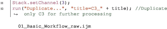
The ImageJ macro file, which you can find in the code repository,² is a simple workflow that runs on an open, active single image. It segments the nuclei (Channel 3, C3) by setting a global automatic threshold, gets the outlines of the single nuclei, and measures the area, in pixels, of each nucleus. Let us see the actual code. There are roughly three steps.

• line 11–12: Duplication of C3 (Nuclei) to isolate the image for further analysis

  

• line 14–20: Filtering C3 and converting it to a binary image for segmentation

  

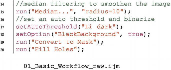
• Line 23: Measuring the area of each nucleus and generating a Results Table, and the ROI Manager listing the outlines of each nucleus. Nuclei that are touching the border of the image are excluded from the measurements.

  

This macro³ does not save any output (binary image, a window with the results, ROI Manager; see Fig. 2.1). They are only visible on the desktop after running the macro. However, it is our aim to save the binary image and the ROI Manager (both as quality control output), as well as the measurement results of each image. We will introduce the saving techniques as we explain each batch processing method below.

Fig. 2.1

The output of the core workflow

Exercise 1

Go through the simple workflow macro 01_Basic_Workflow_raw.ijm line-by-line, analyse each command and make sure to understand what each of them is doing.

2.6 GUI-Based Methods

A very easy method to execute code on an entire set of images is to use the so-called Batch Processor. The Batch Processor is a GUI found under [Process> Batch> Macro...  ].

Fig. 2.2

Batch Processor Interface

Let us have a look on the settings of the Batch Processor (Fig. 2.2).

• 1. Set input and output folder. Input is the folder where you store the images to be processed. Output is where the Processor will automatically store output images. Enter a path for both input and output directories or choose the output via dialog windows by clicking on “Input...”/“Output...”.

• 2. Specify the format for saving the images by the drop-down menu of “Output format”.

• 3. Within the large text field, enter the code to be executed on the images by either copy&pasting to the window, or by opening the simple workflow macro.⁴

• 4. Click the button “Process” to run the code on all images.

While running the batch-processor, we can observe that no image is opened in display; images are processed in the background. Regarding the output, we can find our binary control-images in the output folder, together with one big Results Table containing the measurements of all nuclei of all the (4) images we have worked with. However, ROIs that were in the ROI Manager were not saved.

This nicely shows the power but also the disadvantages of the Batch Processor: it is very fast to run code on an entire set of images, however we do not have full control over what is saved (in this case, the ROIs were not saved). Also, if we would decide to save the, e.g., median filtered image as quality control, this would not be possible. Another disadvantage of the Batch Processor is that it does not handle subfolders, but only processes images on the level of the selected input folder.

2.7 Scripting-Based Methods

In order to have full control over the batch-processing, we need to write all the steps into our full IJ macro script.

2.7.1 Preparing the Code for Batch Processing

Before we execute our code on an entire set of images we want to make sure that the code includes commands to “clean-up” the traces of processing and analysis after each processed image.⁵

• We want to make sure that the ROI Manager does not contain ROIs of another image.

• Depending on the situation we can collect all results in one table or create and save one Results Table for each image. In the latter case we need to clean the Results Table between images.

• We want to close all open images after we analyzed one of the input-images, in order to have a fresh start for the next input image.

In the IJ macro language we can ensure doing so using the following commands for clearing the ROI Manager and Results Table:⁶

To close all images in the end, we can run:

With these “clean-ups”, we are now ready.

2.7.2 ImageJ Macro, IJ1

Now that we have prepared the code for the core workflow, we can work on the script to enable batch-processing. As a starting point for writing, a template of a batch-processing macro is available within the Script Editor under [Templates> ImageJ 1.x> Batch> Process Folder (IJ Macro)].

The template contains three main sections:

• Line 5–7: Getting input folder, output folder and the type of the image to be analyzed;

• Line 15-24: processFolder function registers files to be analyzed and searches also in subfolders;

• Line 26–31: processFile function contains the core workflow processing the individual files.

2.7.2.1 Getting Input Folder, Output Folder

The first several lines of the template (template_Process_Folder.ijm) are utilizing so-called script parameters. For now, we will not use the script parameters and will instead hard-code input directory, output directory and the file suffix. The modified code is in another file, which we will call the macro with hard-coded path.⁷ The script parameters have been commented out and instead input, output, and suffix were specified as follows:

Let us make some remarks related to the path: (1) Make sure to adapt the paths to your local computer; (2) When copied from your system, the path contains either $\backslash$ or /, depending on your operating system. If the path contains a backslash $\backslash$ (older Windows OS) it is best to simply replace it by a slash /. If you want to use a $\backslash$ you need to insert a second backslash: $\backslash \backslash$. This is called an escape character; (3) Instead of $\backslash$ or / you can also use File.separator, which “Returns the file name separator character (/ or $\backslash$)”⁸ that is used by your system.

2.7.2.2 ProcessFolder Function

We have defined the input and output folders, and the suffix (file type). Let us now examine the processFolder function line-by-line. processFolder takes a path as argument. The path points to the folder with the input images, as defined by the user. First, in Line 16, getFileList acquires all the filenames in the directory as an array: each element of this array is a filename, and the length of the array is equal to the number of files within the directory. Array.sort(list) sorts this array in alphanumeric order.

Once we have the sorted list, we loop over it from Line 18, starting at $i=0$ – since the index i of the first element of an array is 0 – until i is smaller than list.length, which gives the number of elements (= number of filenames) in list. For each filename, we create the full path of the file in Line 19 (input + File.separator + list[i]). Note again the usage of File.separator. Once the full path is created, we check whether the path is a directory using the command File.isDirectory. If yes, we call the processFolder function recursively in Line 20. In other words we now take the path of the detected directory as input and repeat the process of getting the FileList and checking each file of this new directory. Only if an item list[i] of our list of filenames is not a directory and endsWith the desired suffix, the function processFile is called. processFile in Line 22 will contain our core workflow and we can finally process and analyze the image. If a file is neither a directory, nor ends with the right file suffix, nothing happens.

Exercise 2

Change the structure of your input folder. Create subfolders and subsubfolders and copy some of the images into them. Rename the images with e.g. “_level1”. Run the Process_Folder.ijm template as it is and follow in which order the files are processed.

2.7.2.3 ProcessFile Function

The function processFile is executed on each file of the desired file type. Within the function, we want to first open an image, then run the core workflow to process and analyze the image, and finally save the output.

For opening a file, we use:

file is the filename stored in list[i] and passed on to the processFile function as the third argument: processFile(input, output, file).

Until this point, we have modified processFile such that it opens an image. For processing the opened image, we can then copy & paste our simple workflow prepared for batch⁹ within the function processFile.

Here you can see the first lines of our core workflow in the function:

Finally, we also want to save the output. Using scripting, we have full control over what to save. In the macro with hard-coded path, you can find the following strategy for saving:¹⁰

• 1. Line 36: Get the pure filename (the file name without the file extension) directly after opening the image. The function on the right-hand side gets “The name of the last file opened with the extension removed”¹¹.

• 2. Line 37: Create a saving prefix string that contains the output folder, the File.separator and the pure filename.

• 3. Lines 66–69:

  

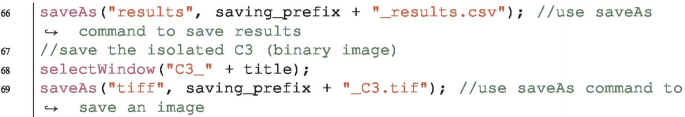
  Save the Results window and the binary image, by using saveAs(format, path). Let us read the documentation of the saveAs command:

  Saves the active image, lookup table, selection, measurement results, selection XY coordinates or text window to the specified file path. The format argument must be “tiff’’, “jpeg’’, “gif’’, “zip’’, “raw’’, “avi’’, “bmp’’, “fits’’, “png’’, “pgm’’, “text image’’, “lut’’, “selection’’, “results’’, “xy Coordinates’’ or “text’’.

  In consequence, for saving the Results window, we use “results” as format, and for saving an image as tif-file, we use “tiff” as format. Note that the active image is the one which is saved, so we need to make sure to activate the binary image by selectWindow("C3_" + title);.

• 4. Save ROIs in the ROI Manager. We use one of the roiManager functions:

  

  It creates a zip file. We can re-open this zip-file afterwards by drag&drop into Fiji: all ROIs will reappear within the ROI Manager. We use the variable saving_prefix that we had built in the step before. It helps us to easily create the paths for the final output-file: we just need to add a suffix and file-ending, e.g. _rois.zip.

2.7.3 Two Different Methods to Get User Input

In the macro with hard-coded path,¹² paths and (file name) suffix are fixed.

This is useful e.g. when we develop a workflow and do not want to interactively select a file every time we run the code.

If we do want to allow for user input, we can devise graphical user interfaces, GUIs, as exemplified in the macro with user interface.¹³

Here getDirectory returns a string with the path pointing to the directory chosen by the user. getString returns a string entered by the user, or the default-string “.tiff” if nothing is changed by the user. The output strings are assigned to the variables input, output or suffix, respectively.

Note that there is also a family of macro commands that starts with Dialog., which allow us to create more complex GUIs for user input. Please refer to the command reference¹⁴ if you are interested in more details.

2.7.3.1 Script parameters

Another option is to use script parameters.¹⁵

Script parameters are by default used in the Process_Folder.ijm batch template – we had replaced them with the actual path in the macro with hard-coded path.¹⁶

#@ initiate any Script Parameter, followed by the Type of variable. #@ File, for example, hands over a path to a file, #@ String a String etc. The appropriate dialog window is automatically generated according to Type. The dialog window can then be further customized using the options within a single parenthesis after #@ Type. As an example, see Line 11 of the code shown above. The options within parentheses specify the message within the dialog box (File suffix) and propose a default value (“.tiff”). You can find more information about script parameters on the ImageJ website.¹⁷

2.7.4 ImageJ Macro, Scijava

Once we use script parameters, we can take advantage of a very convenient way to execute code in batch.

Let us have a look on 03_SciJava.ijm. When we compare it with the script parameter macro with loops,¹⁸ we can see that both contain the same lines for choosing input- and output-folder, and suffix, via script parameters. 03_SciJava.ijm also contains the same commands for saving the output files (Results window, binary image, ROI Manager), as discussed in Sect. 2.7.2. However, 03_SciJava.ijm does not contain any code to batch execute the workflow – neither searching for files, nor looping over several files. To still be able to batch-execute this code, we click “batch” within the Script Editor. The GUI displayed in Fig. 2.3 opens. Select “Input” as parameter to batch and add files to the Input files list.¹⁹ After clicking OK, we see the dialog window for choosing the output directory and the file suffix. Once everything is set, all files listed in the “Input files” field will be processed.²⁰

Fig. 2.3

Interface for selecting input parameters and files

2.7.5 Command-Line Headless Methods

Why do we have script parameters? Macro commands include the getString, getNumber and Dialog family commands that allow us to create a user-interface –  why should we need another way?

This is because script parameters are designed to be generic and universal in terms of interface. This means that the interface for input and output parameters can take any form, including GUI and Command-Line Interface (CLI). As we have seen already, script parameters only declare the type and the name of the variable. How these variables are provided is automatically determined depending on how the macro is called. If you run it with the “Run” button in the Script Editor, the input GUI is automatically generated and shows up on the screen. If you click the “Batch” button, the file names are automatically passed to the variable one-by-one, and images are processed in batch. This is in contrast to the get commands and Dialog commands of the Build-in macro functions, which are limited only to the input via dialog windows.

Now, using this generic and flexible characteristic of script parameters, we can try to run the batch processing macro from command line, without launching Fiji on your desktop. We call this way of running a software “the headless mode”, as the main menu bar (here Fiji) never appears on your screen. This headless usage is especially important when you want to run the macro on a remote server, or a cluster without display.

The command line interface is available in Windows (Git BASH), in Mac OSX (Terminal.app), and in Linux (e.g. Gnome).²¹ The first thing to do is to create a command line alias for Fiji. This can be done with the following command:

Windows

Mac OSX

Linux

In all these cases, <​Path-​to-​Fiji>​ should be replaced by the actual path to Fiji in your local machine. For example, if Fiji is located in the Applications folder of your Mac, the full path to the Fiji executable is:

Then, try the following:

If your alias setting was successful, this command should print all the options that can be used in the CLI for running Fiji.

The second step is to prepare an example batch processing macro. Here, we can take an example from the Script Editor, just like we did in Sect. 2.7.2 Macro IJ1. Open a new Script Editor, and select the menu item [Template> ImageJ 1.x> Batch> Process Folder (IJ1 macro)]. Save the generated example as it is somewhere in your file system. Now, let us just run it from the Script Editor by clicking the “Run” button. You are asked for the locations of an input folder and an output folder, so please choose a folder that contains several TIFF images as the input directory, and choose any folder as the output. After clicking OK, you should see that all TIFF image file names appear printed in the Log window.²²

Using exactly the same script that we tried above, let us run the macro in headless mode. Instead of setting the file paths to input and output folder in the dialog window, we can feed this information as options to the command.²³

Each option sets the following conditions:

• --ij2 : use ImageJ2 instead of ImageJ1;

• --headless : run in headless mode;

• --run $\texttt {<macro> [<arg>]}$ : run <macro> in ImageJ, optionally with arguments separated by comma.

Note how arguments of –$\texttt {run<macro> [<arg>]}$ for paths to input and output folders are set in the above command. Both options are surrounded together by single quotes, and inside them, each path is surrounded by double quotes. The parts surrounded by single quotes are handed over as a single option to the script parameter resolver for macro. Before the execution of the macro, paths specified for variables input and output are separately interpreted as script parameters and used during the macro execution. In this way, options can be nested for different handling.

If you are successful in running the command, the CLI output will list the files from the selected input directory. The code can then be extended just like we have already done in previous sections to include the actual workflow.

Have on mind that macro that work on Desktop (GUI) sometimes fail to work in CLI. This is because some ImageJ functions are tightly associated with GUI and cannot run in the headless mode. For example, a macro that uses the ROI Manager does not work in the headless mode, as the ROI Manager relies heavily on GUI. In such a case, overlays can be used as an alternative to ROIs.

2.8 Collecting Measurement Results During Batch Processing

In this section, we discusses how to collect values that result from analysis of different images. As an example, we will collect the number of detected/analyzed nuclei per image and then calculate the mean and the standard deviation of the number of nuclei per image. We aim for the output of a style: “On average, there were $35.3 \pm 10.5$ nuclei analyzed per image (number of images=4).”.

2.8.1 Collecting Measurements Within an Array

A popular way to collect the measurements is to use an array that is filled with values every time we execute our workflow while iterating over the images. Here, we refer to such an array as “data storage array”. The data collecting macro²⁴ demonstrates the usage of such a data storage array. This macro is based on a macro that we already discussed, the one that uses script parameters and explicitly contains the code for looping.²⁵

We start by creating an empty array in the beginning of the code.

We do not specify the length of the array in this case, which is crucial since at this point of execution IJ has not searched for the files and does not know how many values we will collect.

To now fill the array step-by-step, we execute the following procedure:

• 1. We pass the data storage array collect_nNuclei as input parameter of the function processFolder. Additionally, we introduce the data storage array collect_nNuclei also as the returned value of processFolder. In this way, the data storage array is passed to processFolder, can be modified within the function and then the modified array collect_nNuclei will be returned as output. The final function call looks like this:

  

• 2. We extract the number of analyzed nuclei in each image. As discussed above, processFolder is searching for files (not directories) that end with a defined suffix – “.tiff”. When such a file is found, the function processFile is called. processFile contains the image-processing workflow. We need to modify it in order to extract the number of analyzed nuclei. We get the number of analyzed nuclei by using roiManager(“count”), and take this as the returned value of the processFile function using return:

  

  Note again that we need to change how processFile is called:

  

• 3. In the final step we need to add the output nNuclei to our collecting array collect_nNuclei. This happens within the processFolder function: we extend the collecting array with the new value nNuclei by concatenation.

  

Exercise 3

Explain why we cannot create the data storage array within the processFolder function.

2.8.2 Collecting Measurements Within a Table

Very often we want to collect measurements from different images and save them in a Results Table. We can do so by creating a table, filling it up with the measured values, and once this is done, we can convert the table to an IJ1 Results table. We can easily add summary statistics to an IJ1 Results table using a native function.²⁶

To do this, we first create a table, and initialize an index variable rowIndex for filling up the table.

For adding a value to the table we use:

Finally, in order to use the analysis tools available for a Results table we need to rename the table to “Results”. With this, we can get the summary statistics of measured values:

2.8.3 Collecting Measurements When Using SciJava

In Sect. 2.7.4 we have seen how to utilize the Batch button to conveniently batch execute code using script parameters, without having to explicitly list the files and folders. Similarly, we can collect and output measurements in a very convenient way using script parameters.²⁷ Using the macro 03_SciJava.ijm as start, we only need to add an output parameter and assign our measurement of interest (number of nuclei) to the output variable. The output parameter is defined in the beginning using #@output

The number of nuclei is assigned to nROIs in the end of the workflow:

For each image that we analyze, the output variable nROIs is added to a IJ2/SciJava table that is hidden during the macro execution. This is a different kind of table than the IJ1 Results table, and appears on the desktop when the macro is completed. The table can be saved as CSV file using the menu command [File/Export/Table...]. Just as any CSV file, it can be reopened in Fiji. If you rename the opened CSV file to “Results”, you can also use the summarize-functions to calculate some statistics, as demonstrated in the previous section.

2.9 Application to Bioimage Analysis

Example: Preparing Microscopy Image Files for Visual Inspection

When performing an imaging-based experiment, the first step of the analysis should be a visual inspection of the images. What do you see in the images taken under, or related to, different conditions (e.g. wildtype vs. mutant, treated vs. untreated)? Typical parameters in biology are e.g. changes in intensity of a protein of interest or changes in cell shape. For such an analysis, it is necessary to compare a few, ideally randomly chosen, images reflecting the different conditions side by side. In a standard microscopy experiment, that often means: opening the vendor-format via Bioformats in Fiji, selecting the same plane or channel in all image files, and setting the same brightness and contrast limits for all files. This is time-consuming and error-prone. However, all these steps can be easily recorded using the Command Recorder and then performed on all images in a folder.

We take as an example the 3-channel images already used in this chapter. For easy comparison we:

• Extract the signal channel (Channel 2) by duplication.

• Change the look-up-table (LUT) to gray, since a gray LUT is best inspected by a human eye.

• Set defined values as minimum and maximum contrast. This is essential for comparing the intensities for different images (see also Exercise 3).

These steps can be recorded:²⁸

The only output we aim to save is the contrast-adjusted Channel 2. Therefore, the easiest solution would be to simply copy the code snippet from the Command Recorder to the Batch Processor and execute it after choosing input- and output-folder. The extracted and contrast-enhanced Channel 2 of the different image files are saved to the output folder. These visually enhanced images can then be re-opened in Fiji and easily visually compared. However, when we inspect the saved output files, we observe that they are saved under the same name as the original input files. This bears the risk of errors (e.g. deleting the original files by mistake).

In order to have more control over the saving process it is better to choose the SciJava solution discussed in Sect. 2.7.4. For this we need to specify the input and ask the user to select the output-folder via script parameters. Command open(input) opens the file. We then prepare for easy saving by extracting the filename without file ending. After the short workflow we then save the image and clean-up for the next image. This code runs in batch-mode when clicking on “Batch” within the Script Editor and after adding the files to batch process to the files list (see Fig. 2.3).

Exercise 4

Which command is recorded when you click the “Auto” button in the Brightness/Contrast window? How does this command work and how does it compare to setMinAndMax? Why is it wrong to use “Auto” when we want to compare the intensity of a signal in different images?

Take-Home Message

In Fiji, there are various methods to construct batch-processing workflows. Each method has its own characteristics, advantages and disadvantages, and users can choose ones that best suit their needs in a given situation.

Solutions to the Exercises

Exercise 1

Exercise 2

Folders are processed one after the other. Example of 3 layers of folders (paths shortened for clarity):

Exercise 3

Inside the function processFolder, we call processFolder recursively when the path in list[i] is a directory. This allows the processing of all files in all subfolders. Creating collect_nNuclei by collect_nNuclei = newArray() within the function processFolder would cause overwriting of collect_nNuclei each time when a new subfolder is processed.

Exercise 4

When clicking “Auto” in the Brightness/Contrast window, the following command is recorded: run("Enhance Contrast", "saturated=0.35"). The second arguments indicates that the saturation of pixel values is 0.35, which means that the 0.35% darkest and brightest pixels of the image will all be set to 0 and 65535 (in case of 16-bit image), respectively, by computing appropriate minimum and maximum pixel values to satisfy the requested percentage of pixels to become saturated. At the same time, other pixels with values between these minimum and maximum become scaled linearly. This means that images with different brightness will be scaled differently e.g. a darker image will be enhanced more. Consequently, by applying “auto-contrast”, an image with the maximum value = 500, would look similar to an image with the maximum value of 1500 by different degree of enhancements. Thus, applying auto-contrast is quite misleading if one needs to compare images to inspect the difference in the intensity of a structure, e.g. the expression level of a protein.

To scale and enhance images to the same degree, we can specify the minimum and the maximum values by using setMinAndMax(0, 2000). With this command, we are scaling all images using fixed limits (minimum and maximum pixel values) and by that we can compare the images after the enhancement. Note that these limits should fit within the range of all pixel values in all images.

References

Li CH, Tam PKS (1998) An iterative algorithm for minimum cross entropy thresholding. Pattern Recognit Lett 19(8):771–776
Miura K, Tosi S, Möhl C, Zhang C, Paul-Gilloteaux P, Schultz U, Nørrelykke SF, Tischer C, Pengo, T (2016) Bioimage Data Analysis. Wiley-VCH, Weinheim. http://www.imaging-git.com/applications/bioimage-data-analysis-0
Rueden CT, Schindelin J, Hiner MC, DeZonia BE, Walter AE, Arena ET, Eliceiri KW (2017) ImageJ2: ImageJ for the next generation of scientific image data. BMC Bioinform 18(1):529. https://doi.org/10.1186/s12859-017-1934-z
Schindelin J, Arganda-Carreras I, Frise E, Kaynig V, Longair M, Pietzsch T, Preibisch S, Rueden C, Saalfeld S, Schmid B, Tinevez J-Y, White DJ, Hartenstein V, Eliceiri K, Tomancak P, Cardona A (2012) Fiji: an open-source platform for biological-image analysis. Nat Methods 9(7):676–682. Publisher: Nature Publishing Group, a division of Macmillan Publishers Limited. All Rights Reserved. https://doi.org/10.1038/nmeth.2019
Schneider CA, Rasband WS, Eliceiri KW (2012) NIH Image to ImageJ: 25 years of image analysis. Nat Methods 9(7):671–675. Publisher: Nature Publishing Group ISBN: 1548-7091. http://www.nature.com/doifinder/10.1038/nmeth.2089
Acknowledgements
Images were recorded with the help of Susanne Hasse, Mihail Sarov lab, MPI-CBG, Dresden, Germany. We thank Jan Eglinger (FMI Basel, Switzerland) for thoroughly reading the text, testing the code, and giving valuable suggestions for further improvements.
Author information
Authors and Affiliations
Editor information
Editors and Affiliations
Rights and permissions
Open Access This chapter is licensed under the terms of the Creative Commons Attribution 4.0 International License (http://creativecommons.org/licenses/by/4.0/), which permits use, sharing, adaptation, distribution and reproduction in any medium or format, as long as you give appropriate credit to the original author(s) and the source, provide a link to the Creative Commons license and indicate if changes were made.
The images or other third party material in this chapter are included in the chapter's Creative Commons license, unless indicated otherwise in a credit line to the material. If material is not included in the chapter's Creative Commons license and your intended use is not permitted by statutory regulation or exceeds the permitted use, you will need to obtain permission directly from the copyright holder.
Copyright information
© 2022 The Author(s)
About this chapter
Cite this chapter
Klemm, A., Miura, K. (2022). Batch Processing Methods in ImageJ. In: Miura, K., Sladoje, N. (eds) Bioimage Data Analysis Workflows ‒ Advanced Components and Methods . Learning Materials in Biosciences. Springer, Cham. https://doi.org/10.1007/978-3-030-76394-7_2
Download citation
DOI: https://doi.org/10.1007/978-3-030-76394-7_2
Published:
Publisher Name: Springer, Cham
Print ISBN: 978-3-030-76393-0
Online ISBN: 978-3-030-76394-7
eBook Packages: Biomedical and Life SciencesBiomedical and Life Sciences (R0)