Sentiment Analysis of Financial News: Mechanics and Statistics

Abstract

This chapter describes the basic mechanics for building a forecasting model that uses as input sentiment indicators derived from textual data. In addition, as we focus our target of predictions on financial time series, we present a set of stylized empirical facts describing the statistical properties of lexicon-based sentiment indicators extracted from news on financial markets. Examples of these modeling methods and statistical hypothesis tests are provided on real data. The general goal is to provide guidelines for financial practitioners for the proper construction and interpretation of their own time-dependent numerical information representing public perception toward companies, stocks’ prices, and financial markets in general.

1 Introduction

Nowadays several news technology companies offer sentiment data to assist the financial trading industry into the manufacturing of financial news sentiment indicators to feed as information to their automatic trading systems and for the making of investment decisions. Manufacturers of news sentiment-based trading models are faced with the problem of understanding and measuring the relationships among sentiment data and their financial goals, and further translating these into their forecasting models in a way that truly enhances their predictive power.

Some issues that arise when dealing with sentiment data are: What are the sentiment data—based on news of a particular company or stock—saying about that company? How can this information be aggregated to a forecasting model or a trading strategy for the stock? Practitioners apply several ad hoc filters, as moving averages, exponential smoothers, and many other transformations to their sentiment data to concoct different indicators in order to exploit the possible dependence relation with the price or returns, or any other observable statistics. It is then of utmost importance to understand why a certain construct of a sentiment indicator might work or not, and for that matter it is crucial to understand the statistical nature of indicators based on sentiment data and analyze their insertion in econometric models. Therefore, we consider two main topics in sentiment analysis: the mechanics, or methodologies for constructing sentiment indicators, and the statistics, including stylized empirical facts about these variables and usage in price modeling.

The main purpose of this chapter is to give guidelines to users of sentiment data on the elements to consider in building sentiment indicators. The emphasis is on sentiment data extracted from financial news, with the aim of using the sentiment indicators for financial forecasting. Our general focus is on sentiment analysis for English texts. As a way of example, we apply this fundamental knowledge to construct six dictionary-based sentimental indicators and a ratio of stock’s news volume. These are obtained by text mining streams of news articles from the Dow Jones Newswires (DJN), one of the most actively monitored source of financial news today. In the Empirical section (Sect. 4) we describe these sentimental and volume indicators, and further in the Statistics section (Sect. 3) analyze their statistical properties and predictive power for returns, volatility, and trading volume.

1.1 Brief Background on Sentiment Analysis in Finance

Extensive research literature in behavioral finance has shown evidence to the fact that investors do react to news. Usually, they show greater propensity for making an investment move based on bad news rather than on good news (e.g., as a general trait of human psychology [5, 39] or due to specific investors’ trading attitudes [17]). Li [27] and Davis et al. [11] analyze the tone of qualitative information using term-specific word counts from corporate annual reports and earnings press releases, respectively. They go on to examine, from different perspectives, the contemporaneous relationships between future stock returns and the qualitative information extracted from texts of publicly available documents. Li finds that the two words “risk” and “uncertain” in firms’ annual reports predict low annual earnings and stock returns, which the author interprets as under-reaction to “risk sentiment.” Tetlock et al. [45] examine qualitative information in news stories at daily horizons and find that the fraction of negative words in firm-specific news stories forecasts low firm earnings. Loughran and McDonald [29] worked out particular lists of words specific to finance, extracted from 10-K filings, and tested whether these lists actually gauge tone. The authors found significant relations between their lists of words and returns, trading volume, subsequent return volatility, and unexpected earnings. These findings are corroborated by Jegadeesh and Wu [24] who designed a measure to quantify document tone and found significant relation between the tone of 10-Ks and market reaction for both negative and positive words. The important corollary of these works is that special attention should be taken to the nature and contents of the textual data used for sentiment analysis intended for financial applications. The selection of documents from where to build a basic lexicon has major influence on the accuracy of the final forecasting model, as sentiment varies according to context, and lists of words extracted from popular newspapers or social networks convey emotions differently than words from financial texts.

2 Mechanics of Textual Sentiment Analysis

We focus our exposition on sentiment analysis of text at the aspect level. This means that our concern is to determine whether a document, or a sentence within a document, expresses a positive, negative, or other sentiment emotions toward a target. For other levels and data corpuses, consult the textbook by Bing Liu [28].

In financial applications, the targets are companies, financial markets, commodities, or any other entity with financial value. We then use this sentiment information to feed forecasting models of variables quantifying the behavior of the financial entities of interest, e.g., price returns, volatility, and financial indicators.

A typical workflow for building forecasting models based on textual data goes through the following stages: (i) textual corpus creation and processing, (ii) sentiment computation, (iii) sentiment scores aggregation, and (iv) modeling.

• (i) Textual corpus management. The first stage concerns the collecting of textual data and applying text mining techniques to clean and categorize terms within each document. We assume texts come in electronic format and that each document has a unique identifier (e.g., a filename) and a timestamp. Also, that through whatever categorization scheme used, we have identified within each document the targets of interest. Thus, documents can be grouped by common target and it is possible that a document appears in two different groups pertaining to two different targets.

Example 1

Targets (e.g., a company name or stock ticker) can be identified by keyword matching or name entity recognition techniques (check out the Stanford NER software.¹) Alternatively, some news providers like Dow Jones Newswires include labels in their xml files indicating the company that the news is about.

• (ii) Computing sentiment scores. Sentiment analysis is basically a text classification problem. Hence, one can tackle this algorithmic problem by either 1) applying a supervised machine learning algorithm that is trained on text already labeled as positive or negative (or any other emotion) or 2) using an unsupervised classification method based on the recognition of some fixed syntactic patterns, or words, that are known to express a sentiment (sentiment lexicon). The latter is frequently used by researchers and practitioners in Finance, and it is the one applied on the data we have at hand for sentiment analysis in this work. Hence, we will prioritize the exposition of the lexicon-based unsupervised method and just give some pointers to the literature in the machine learning approach to sentiment classification.

• (ii.A) Lexicon-based unsupervised sentiment classification. The key component of this text classification method is a dictionary of words, and more general, syntactic patterns, that denote a specific sentiment. For example, positiveness is conveyed by words such as good, admirable, better, etc. and emoticons such as :-) or ; -] and alike, often used in short messages like those in Twitter [8, 19]. These groups of words conform a sentiment lexicon or dictionary.

Given a fixed sentiment $\mathscr S$ (e.g., positive, negative, …), determined by some lexicon $L(\mathscr {S})$, a basic algorithm to assign a $\mathscr S$-sentiment score to a document is to count the number of appearances of terms from $L(\mathscr {S})$ in the document. This number gives a measure of the strength of sentiment $\mathscr S$ in the document. In order to compare the strengths of two different sentiments in a document, it would be advisable to relativize these numbers to the total number of terms in the document. There are many enhancements of this basic sentiment scoring function, according to the different values given to the terms in the lexicon (instead of each having an equal value of 1), or if sign is considered to quantify direction of sentiment, and further considerations on the context where, depending on neighboring words, the lexicon terms may change their values or even shift from one sentiment to another. For example, good is positive, but not good is negative. We shall revise some of these variants, but for a detailed exposition, see the textbook by Liu [28] and references therein.

Let us now formalize a general scheme for a lexicon-based computation of a time series of sentiment scores for documents with respect to a specific target (e.g., a company or a financial security). We have at hand λ = 1, …, Λ lexicons L _λ, each defining a sentiment. We have K possible targets and we collect a stream of documents at different times t = 1, …, T. Let N _t be the total number of documents with timestamp t. Let D _n,t,k be the n-th document with timestamp t and make mention of the k-th target, for n = 1, …, N _t, t = 1, …, T and k = 1, …, K.

Fix a lexicon L _λ and target G _k. A sentiment score based on lexicon L _λ for document D _n,t,k relative to target G _k can be defined as

$$\displaystyle \begin{aligned} S_{n,t}(\lambda,k) = \sum_{i=1}^{I_d} w_i S_{i,n,t}(\lambda,k) \end{aligned} $$

(1)

where S _i,n,t(λ, k) is the sentiment value given to unigram i appearing in the document and according to lexicon L _λ, being this value zero if the unigram is not in the lexicon. I _d is the total number of unigrams in the document D _n,t,k and w _i is a weight, for each unigram that determines the way sentiment scores are aggregated in the document.

Example 2

If S _i,n,t = 1 (or 0 if unigram i is not in the lexicon), for all i, and w _i = 1∕I _d, we have the basic sentiment density estimation used in [27, 29, 45] and several other works on text sentiment analysis, giving equal importance to all unigrams in the lexicon. A more refined weighting scheme, which reflects different levels of relevance of the unigram with respect to the target, is to consider w _i = dist(i, k)⁻¹, where dist(i, k) is a word distance between unigram i and target k [16].

The sentiment score S _i,n,t can take values in $\mathbb {R}$ and be decomposed into factors v _i ⋅ s _i, where v _i is a value that accounts for a shift of sentiment (a valence shifter: a word that changes sentiments to the opposite direction) and s _i the sentiment value per se.

• (ii.A.1) On valence shifters. Originally proposed and analyzed their contrarian effect on textual sentiment in [34], these are words that can alter a polarized word’s meaning and belong to one of four basic categories: negators, amplifiers, de-amplifiers, and adversative conjunction. A negator reverses the sign of a polarized word, as in “that company is not good investment.” An amplifier intensifies the polarity of a sentence, as, for example, the adverb definitively amplifies the negativity in the previous example: “that company is definitively not good investment.” De-amplifiers (also known as downtowners), on the other hand, decrease the intensity of a polarized word (e.g., “the company is barely good as investment”). An adversative conjunction overrules the precedent clause’s sentiment polarity, e.g., “I like the company but it is not worthy.”

Shall we care about valence shifters? If valence shifters occur frequently in our textual datasets, then not considering them in the computation of sentiment scores in Eq. (1) will render an inaccurate sentiment valuation of the text. More so in the case of negators and adversative conjunctions which reverse or overrule the sentiment polarity of the sentence. For text from social networks such as Twitter or Facebook, the occurrence of valence shifters, particularly negators, has been observed to be considerably high (approximately 20% for several trending topics²), so certainly their presence should be considered in Eq. (1).

We have computed the appearance of valence shifters in a sample of 1.5 million documents from the Dow Jones Newswires set. The results of these calculations, which can be seen in Table 1, show low occurrence of downtoners and adversatives (around 3%), but negators in a number that may be worth some attention.

Table 1 Occurrence % of valence shifters in 1.5 MM DJN documents

• (ii.A.2) Creating lexicons. A starting point to compile a set of sentiment words is to use a structured dictionary (preferably online as WordNet) that lists synonyms and antonyms for each word. Then begin with a few selected words (keywords) carrying a specific sentiment and continue by adding some of the synonyms to the set, and to the complementary sentimental set add the antonyms. There are many clever ways of doing this sentiment keyword expansion using some supervised classification algorithms to find more words carrying similar emotion. An example is the work of Tsai and Tang [48] on financial keyword expansion using the continuous bag-of-words model on the 10-K mandated annual financial reports. Another clever supervised scheme based on network theory to construct lexicons is given in [35]. For a more extensive account of sentiment lexicon generation, see [28, Chap. 7] and the many references therein.

• (ii.B) Machine learning-based supervised sentiment classification. Another way to classify texts is by using machine learning algorithms, which rely on a previously trained model to generate predictions. Unlike the lexicon-based method, these algorithms are not programmed to respond in a certain way according to the inputs received, but to extract behavior patterns from pre-labeled training datasets. The internal algorithms that shape the basis of this learning process have some strong statistical and mathematical components. Some of the most popular are Naïve Bayes, Support Vector Machines, and Deep Learning. The general stages of textual sentiment classification using machine learning models are the following:

  Corpus development and preprocessing. The learning process starts from a manually classified corpus that after feature extraction will be used by the machine learning algorithm to find the best fitted parameters and asses the accuracy in a test stage. This is why the most important part for this process is the development of a good training corpus. It should be as large as possible and be representative of the set of data to be analyzed. After getting the corpus, techniques must be applied to reduce the noise generated by sentiment meaningless words, as well as to increase the frequency of each term through stemming or lemmatization. These techniques depend on the context to which it is applied. This means that a model trained to classify texts from a certain field could not be directly applied to another. It is then of key importance to have a manually classified corpus as good as possible.

  Feature extraction. The general approach for extracting features consists of transforming the preprocessed text into a mathematical expression based on the detection of the co-occurrence of words or phrases. Intuitively, the text is broken down into a series of features, each one corresponding to an element of the input text.

  Classification. During this stage, the trained model receives an unseen set of features in order to obtain an estimated class.

  For further details, see [40, 28].

  An example of sentiment analysis machine learning method is Deep-MLSA [13, 12]. This model consists of a multi-layer convolutional neural network classifier with three states corresponding to negative, neutral, and positive sentiments. Deep-MLSA copes very well with the short and informal character of social media tweets and has won the message polarity classification subtask of task 4 “Sentiment Analysis in Twitter” in the SemEval competition [33].

• (iii) Methods to aggregate sentiment scores to build indicators. Fix a lexicon L _λ and target G _k. Once sentiment scores for each document related to target G _k are computed following the routine described in Eq. (1), proceed to aggregate these for each timestamp t to obtain the L _λ-based sentiment score for G _k at time t, denoted by S _t(λ, k):

  $$\displaystyle \begin{aligned} S_t(\lambda,k) = \sum_{n=1}^{N_t} \beta_n S_{n,t}(\lambda,k) \end{aligned} $$

  (2)

  As in Eq. (1), the weights β _n determine the way the sentiment scores for each document are aggregated. For example, considering β _n = 1∕length(D _n,t,k) would give more relevance to short documents.

  We obtain in this way a time series of sentiment scores, or sentiment indicator, {S _t : t = 1, …T}, based on lexicon L _λ that defines a specific sentiment for target G _k. Variants of this L _λ-based sentiment indicator for G _k can be obtained by applying some filters F to S _t, thus {F(S _t) : t = 1, …T}. For instance, apply a moving average to obtain a smoothed version of the raw sentiment scores series.

• (iv) Modeling. Consider two basic approaches: either use the sentiment indicators as exogenous features for forecasting models, and test their relevance in forecasting price movements, returns of price, or other statistics of the price, or use them as external advisors for ranking the subjects (targets) of the news—which in our case are stocks—and create a portfolio. A few selected examples from the vast amount of published research on the subject of forecasting and portfolio management with sentiment data are [3, 4, 6, 21, 29, 44, 45, 49].

  For a more extensive treatment of the building blocks for producing models based on textual data, see [1] and the tutorial for the sentometrics package in [2].

3 Statistics of Sentiment Indicators

In this second part of the chapter, we present some observed properties of the empirical data used in financial textual sentiment analysis, and statistical methods commonly used in empirical finance to help the researchers gain insight on the data for the purpose of building forecasting models or trading systems.

These empirical properties, or stylized facts, reported in different research papers, seem to be caused by and have an effect mostly on retail investors, according to a study by Kumar and Lee [26]. For it is accepted that institutional investors are informationally more rational in their trading behaviors (in great part due to a higher automatization of their trading processes and decision making), and consequently it is the retail investor who is more affected by sentiment tone in financial news and more prone to act on it, causing stock prices to drift away from their fundamental values. Therefore, it is important to keep in mind that financial text sentiment analysis and its applications would make more sense on markets with a high participation of retail investors (mostly from developed economies, such as the USA and Europe), as opposed to emerging markets. In these developed markets, institutional investors could still exploit the departures of stock prices from fundamental values because of the news-driven behavior of retail investors.

3.1 Stylized Facts

We list the most often observed properties of news sentiment data relative to market movements found in studies of different markets and financial instruments and at different time periods.

1. Volume of news and volatility correlation. :

The longer the stock is on the news, the greater its volatility. This dependency among volume of news on a stock and its volatility has been observed for various stocks, markets, and for different text sources. For example, this relation has been observed with text data extracted from Twitter and stocks trading in S&P 500 in [3].

2. Larger volume of news near earnings announcement dates. :

The volume of news about a company tends to increase significantly in the days surrounding the company’s earnings announcement. This fact was observed by Tetlock, Saar-Tsechansky, and Macskassy in [45] for news appearing in Wall Street Journal and Dow Jones Newswires from 1980 to 2004, for companies trading in the S&P 500 index. The authors produced a histogram outlining the relationship between the number of company-specific news and the number of days since (respectively, until) the company’s last (respectively, next) earnings announcement (which is the 0 in the plot). The authors did this for all companies collectively; we will update this histogram and show particular cases for individual companies.

This fact suggests a possible statistical dependency relation among company-specific news and company’s fundamentals.

3. Negative sentiments are more related to market movements than positive :

ones. This is observed in, e.g., [3, 29, 45] and [10], although the latter for data in the pre-Internet era, and the phenomenon is most prominent for mid and small-cap stocks.

4. Stronger effects observed for mid and small-capitalization stocks. :

This is suggested and analyzed in [10]. It is related to the fact that retail investors are those who mostly trade based on news sentiment, and this type of investors does not move big-cap stocks.

3.2 Statistical Tests and Models

In order to make some inference and modeling, and not remain confined to descriptive statistics, several tests on the indices, the targets, and their relationships can be performed. Also, models and model selection can be attempted.

3.2.1 Independence

Previous to using any indicator as a predictor, it is important to determine whether there is some dependency, in a statistical sense, among the target Y  and the predictor X. We propose the use of an independence test based on the notion of distance correlation, introduced by Szekely et al. [43].

Given random variables X and Y  (possibly multivariate), from a sample (X ₁, Y ₁), …, (X _n, Y _n), the distance correlation is computed through the following steps:

• 1. Compute all Euclidean distances among pairs of observations of each vector ∥X _i − X _j∥ and ∥Y _i − Y _j∥ to get 2 n × n distance matrices, one for each vector.

• 2. Double-center each element: to each element, subtract the mean of its row and the mean of its column, and add the matrix mean.

• 3. Finally, compute the covariance of the n ² centered distances.

Distance correlation is obtained by normalizing in such a way that, when computed with X = Y , the result is 1. It can be shown that, as n →∞, the distance covariance converges to a value that vanishes if and only if the vectors X and Y  are independent. In fact, the limit is a certain distance between the characteristic function φ _{(X,Y )} of the joint vector (X, Y ) and the product of the characteristic functions of X and Y , φ _X φ _Y. From this description, some of the advantages of the distance correlation are clear: it can be computed for vectors, not only for scalars; it characterizes independence; since it is based on distances, X and Y  can have different dimensions—we can detect dependencies between two groups, one formed by p variables and the other by q; and it is rotation-invariant.

The test of independence consists of testing the null hypothesis of zero distance correlation. The p-values are obtained by bootstrap techniques. The R package energy [38] includes the functions dcor and dcor.test for computing the distance correlation and the test of independence.

3.2.2 Stationarity

In the context of economic and/or social variables, we typically only observe one realization of the underlying stochastic process defining the different variables. It is not possible to obtain successive samples or independent realizations of it. In order to be able to estimate the “transversal” characteristics of the process, such as mean and variance, from its “longitudinal” evolution, we must assume that the transversal properties (distribution of the variables at each instant in time) are stable over time. This leads to the concept of stationarity.

A stochastic process (time series) is stationary (or strictly stationary) if the marginal distributions of all the variables are identical and the finite-dimensional distributions of any arbitrary set of variables depend only on the lags that separate them. In particular, the mean and the variance of all the variables are the same. Moreover, the joint distribution of any set of variables is translation-invariant (in time). Since in most cases of time series the joint distributions are very complicated (unless the data come from a very simple mechanism, such as i.i.d. observations), a usual procedure is to specify only the first- and second-order moments of the joint distributions, that is, E X _t and EX _t+h X _t for t = 1, 2, …, h = 0, 1, …, focusing on properties that depend only on these. A time series is weakly stationary if EX _t is constant and EX _t+h X _t only depends on h (but not on t). This form of stationarity is the one that we shall be concerned with.

Stationarity of a time series can sometimes be assessed through Dickey–Fuller test [14], which is not exactly a test of the null hypothesis of stationarity, but rather a test for the existence of a unit root in autoregressive processes. The alternative hypothesis can either be that the process is stationary or that it is trend-stationary (i.e., stationary after the removal of a trend).

3.2.3 Causality

It is also important to assess the possibility of causation (and not just dependency) of a random process X _t toward another random process Y _t. In our case X _t being a sentiment index time series and Y _t being the stock’s price return, or any other functional form of the price that we aim to forecast. The basic idea of causality is that due to Granger [20] which states that X _t causes Y _t, if Y _t+k, for some k > 0 can be better predicted using the past of both X _t and Y _t than it can by using the past of Y _t alone. This can be formally tested by considering a bivariate linear autoregressive model on X _t and Y _t, making Y _t dependent on both the histories of X _t and Y _t, together with a linear autoregressive model on Y _t, and then test for the null hypothesis of “X does not cause Y ,” which amounts to a test that all coefficients accompanying the lagged observations of X in the bivariate linear autoregressive model are zero. Then, assuming a normal distribution for the data, we can evaluate the null hypothesis through an F-test. This augmented vector autoregressive model for testing Granger causality is due to Toda and Yamamoto [47] and has the advantage of performing well with possibly non-stationary series.

There are several recent approaches to testing causality based on nonparametric methods, kernel methods, and information theory, among others, that cope with nonlinearity and non-stationarity, but disregarding the presence of side information (conditional causality); see, for example, [15, 30, 50]. For a test of conditional causality, see [41].

3.2.4 Variable Selection

The causality analysis reveals any cause–effect relationship between the sentiment indicators and any of the securities’ price function as target. A next step is to analyze these sentiment indicators, individually or in an ensemble, as features in a regression model for any of the financial targets. A rationale for putting variables together could be at the very least what they might have in common semantically. For example, joint together in a model, all variables express a bearish (e.g., negativity) or bullish (e.g., positivity) sentiment. Nonetheless, at any one period of time, not all features in one of these groups might cause the target as well as their companions, and their addition in the model might add noise instead of value information. Hence, a regression model which discriminates the importance of variables is in order.

Here is where we propose to do a LASSO regression with all variables under consideration that explain the target. The LASSO, due to Tibshirani [46], optimizes the mean square error of the target and linear combination of the regressors, subject to a L ₁ penalty on the coefficients of the regressors, which amounts to eliminating those which are significantly small, hence removing those variables that contribute little to the model. The LASSO does not take into account possible linear dependencies among the predictors that can lead to numerical unstabilities, so we recommend the previous verification that no highly correlated predictors are considered together. Alternatively, adding a L ₂ penalty on the coefficients of the regressors can be attempted, leading to an elastic net.

4 Empirical Analysis

Now we put into practice the lessons learned so far.

A Set of Dictionary-Based Sentiment Indicators

Combining the lexicons defined by Loughran and McDonald for [29] with extra keywords manually selected, we build six lexicons. For each one of these lexicons, and each company trading in the New York Stock Exchange market, we apply Eq. (1) to compute a sentiment score for each document extracted from a dataset of Dow Jones Newswires in the range of 1/1/2012 to 31/12/2019. We aggregate these sentiment scores on an hourly and a daily basis using Eq. (2) and end up with 2 × 6 hourly and daily period time series of news sentiment values for each NYSE stock. These hourly and daily sentiment indicators are meant to convey the following emotions: positive, Financial Up (finup), Financial Hype (finhype), negative, Financial Down (findown), and fear. Additionally, we created daily time series of the rate of volume of news referring to a stock with respect to all news collected within the same time frame. We termed this volume of news indicator as Relative Volume of Talk (RVT).

We use historic price data of a collection of stocks and their corresponding sentiment and news volume indicators (positive, finup, finhype, negative, fear, findown, and RVT) to verify the stylized facts of sentiment on financial securities and check the statistical properties and predictive power of the sentiment indicators to returns (ret), squared returns (ret2, as a proxy of volatility), and rate of change of trading volume (rVol). We sample price data with daily frequency from 2012 to 2019 and with hourly frequency (for high frequency tests) from 11/2015 to 11/2019. For each year we select the 50 stocks from the New York Stock Exchange market that have the largest volume of news to guarantee sufficient news data for the sentiment indicators. Due to space limitations, in the exhibits we present the results for 6 stocks from our dataset representatives of different industries: Walmart (WMT), Royal Bank of Scotland (RBS), Google (GOOG), General Motors (GM), General Electric (GE), and Apple Inc. (AAPL).

Stylized fact 1. :

We have observed, through independence tests based on distance correlation, that during relatively long periods of time, ret2, a proxy of volatility, and our RVT index are dependent variables, in particular, for “mediatic” companies, such as Amazon, Google, Apple, and blue chips in general. This is illustrated in Fig. 2.

Stylized fact 2. :

We take on the graphical idea of Tetlock et al. [45] representing the relation of news volume to earnings announcement date. However, instead of the bar plot of accumulated volumes for each date, we propose a more informative graphical representation of the distribution of the daily accumulated volumes of news (Fig. 1). This is constructed by drawing the boxplots [31] of volumes of news rather than its simple aggregation on the earning’s day and previous/successive days. Moreover, since the effect of news on financial market behavior (and its reciprocal) around earnings announcement is noticeable only for short periods, we reduce the scope of analysis to 25 days after and before earnings announcement days (which are all placed as the 0 of the plot) and thus consider each news once (either as preceding or succeeding an earnings announcement).

Fig. 1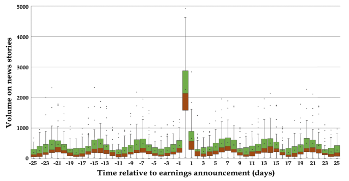

Volume of news around earnings announcements. As in [45] we consider all firm-specific news stories about S&P 500 firms that appear in Dow Jones Newswires from 2012 to 2019, but consider a shorter range of 25 days before and 25 days after earnings announcements (time 0). For each news story, we compute the number of days until the corresponding firm’s next earnings announcement or the number of days after the firm’s last earnings announcement. Each story contributes only once to the volume of news t ∈ [−25, 25] days away to or from the earnings announcement, and we plot a boxplot of this volume variable at each period t of days

Fig. 2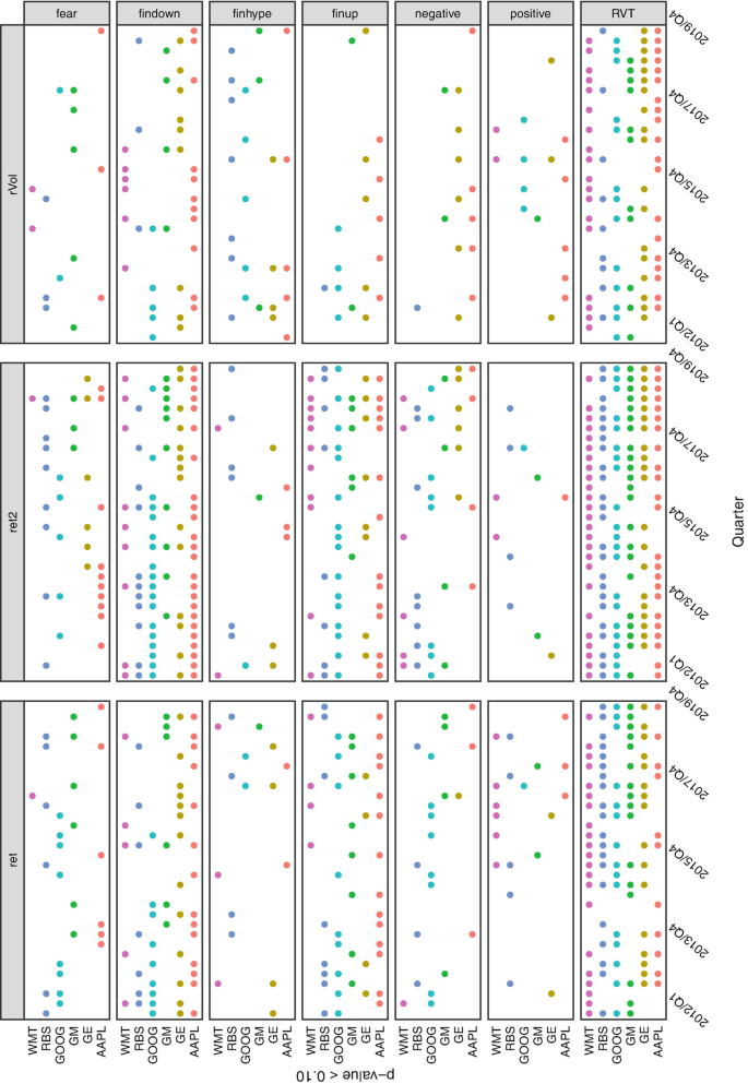

Dependency through distance correlation tests (significance level at 0.1) performed on quarterly windows of daily data from 2012 to 2019

In all the periods, the distribution of the number of news is highly asymmetric (all means are larger than medians), and their right tails are heavy, except on earning’s day itself, where it looks more symmetric. From this new plot, we can see that, not only on earnings day but 1 and 2 weeks before and after earnings day, there is a rise in the volume of news. The most prominent increase in volume of news is seen the exact day of earnings announcement, and the day immediately after earnings announcement has also an abnormal increase with respect to the rest of the series of volumes, indicating a flourish of after-the-facts news. The number of extreme observations of each day is small: at most five companies exceed the standard limit (1.5 times the inter-quartile range) for declaring the value an “outlier”.

We cannot then conclude from our representation of the media coverage of earnings announcements that the sentiments in the news may forecast fundamental indicators of the health of a company (e.g., price-to-earnings, price-to-book value, etc.) as it is done in [45], except perhaps for the few most talk-about companies, the outliers in our plot. However, we do speculate that the sentiment in the news following earnings announcements is the type of information useful for trading short sellers, as such has been considered in [17].

Stylized fact 3. :

Again by testing independence among sentiment indices and market indicators (specifically, returns and squared returns), we have observed in our experiments that most of the time, sentiment indices related to negative emotions show dependency with ret and ret2 (mostly Financial Down and less intensive negative) more often than sentiment indices carrying positive emotions. This is illustrated in Fig. 2.

Independence and Variable Selection

The distance correlation independence tests are exhibited in Fig. 2 and the results from LASSO regressions in Fig. 3. From these we observed the consistency of LASSO selection with dependence/independence among features and targets. The most sustained dependencies through time, and for the majority of stocks analyzed, are observed between RVT and ret2, RVT and rVol, findown and ret2, and finup and ret. LASSO selects RVT consistently with dependence results in the same long periods as a predictor of both targets ret2 and rVol, and it selects findown often as a predictor of ret2, and finup as a predictor of ret. On the other hand, positive is seldom selected by LASSO, just as this sentiment indicator results independent most of the time to all targets.

Fig. 3

Selected variables by LASSO tests performed on quarterly windows of daily data from 2012 to 2019

Stationarity

Most of the indices we have studied follow some short-memory stationary processes. Most of them are Moving Averages, indicating dependency on the noise component, not on the value of the index, and always at small lags, at most 2.

Causality

We have performed Granger causality tests on sentiment data with the corresponding stock’s returns, squared returns, and trading volumes as the targets. We have considered the following cases:

• Data with daily frequency, performing the tests on monthly windows within the 2012–2019 period.

• Data with hourly frequency ranging from November 2015 to November 2019. In this case, we evaluated on both daily and weekly windows. Additionally, for the weekly windows, an additional test was run with overlapping windows starting every day.

In both cases, we find that for almost all variables, the tests only find causality in roughly 5% of the observations, which corresponds to the p-value (0.05) of the test. This means that the number of instances where causality is observed corresponds to the expected number of false positives, which would suggest that there is no actual causality between the sentiment indicators and the targets. The only pair of sentiment variable and target that consistently surpasses this value is RVT and ret2, for which causality is found in around 10% of the observations of daily frequency data (see Fig. 4).

Fig. 4

Total success rate of the causality tests (significance level at 0.05) performed on monthly windows of daily data of the 2012–2019 period, across all stocks considered

Nonetheless, the lack of causality does not imply the lack of predictive power of the different features for the targets, only that the models will not have a causal interpretation in economic terms. Bear in mind that causality (being deterministic) is a stronger form of dependency and subsumes predictability (a random phenomenon).

5 Software

R

There has been a recent upsurge in R packages specific for topic modeling and sentiment analysis. The user has nowadays at hand several built-in functions in R to gauge sentiment in texts and construct his own sentiment indicators. We make a brief review below of the available R tools exclusively tailored for textual sentiment analysis. This list is by no means exhaustive, as new updates are quickly created due to the growing interest in the field, and that other sentiment analysis tools are already implicitly included in more general text mining packages as tm [32], openNLP [22], and qdap [37]. In fact, most of the current packages specific for sentiment analysis have strong dependencies on the aforementioned text mining infrastructures, as well as others from the CRAN Task View on Natural Language Processing³

SentimentAnalysis (2019-03)::

Performs a sentiment analysis of textual contents in R. Incorporates various existing dictionaries (e.g., Harvard IV or finance-specific dictionaries such as Loughran-McDonald), and it can also create customized dictionaries. The latter uses LASSO regularization as a statistical approach to select relevant terms based on an exogenous response variable [18].

RSentiment (2018-07)::

Analyzes the sentiment of a sentence in English and assigns score to it. It can classify the sentences to the following categories of sentiments: positive, negative, very positive, very negative, and neutral. For a vector of sentences, it counts the number of sentences in each category of sentiment. In calculating the score, negation and various degrees of adjectives are taken into consideration [9].

sentimentr (2019-03)::

Calculates text polarity sentiment [36].

sentometrics (2019-11)::

An integrated framework for textual sentiment time series aggregation and prediction. It contains all of the functions necessary to implement each one of the stages in the workflow described in Sect. 2 for building news sentiment-based forecasting models [2].

quanteda (2019-11)::

Quantitative analysis of textual data [7].

syuzhet (2017)::

Extracts sentiment and sentiment-derived plot arcs from the text [25].

Python

For Python’s programmers there are also a large number of options for sentiment analysis. In fact, a quick search for “Sentiment Analysis” on The Python Package Index (PyPI)⁴ returns about 6000 items. Here we include a reduced list of the most relevant modules.

Vader::

Valence Aware Dictionary for sEntiment Reasoning is a rule-based model [23], mainly trained on the analysis of social texts (e.g., social media texts, movie reviews, etc.). Vader classifies the sentences in three categories: positive, negative, and neutral representing the ratios of proportions of text that fall into each category (the summation is 1 or close). It also provides a compound score which is computed by summing the valence scores of each word in the lexicon; this value is normalized between − 1 and 1.⁵ An implementation of Vader can also be found in the general-purpose library for Natural Language Processing nltk.

TextBlob::

From a given input text, the library⁶ computes the sentiment in terms of polarity and subjectivity scores lying on the ranges [−1.0, 1.0] and [0.0, 1.0], respectively. For the subjectivity scores 0 means very objective and 1 is very subjective.

Pattern::

It is a multipurpose package for web mining, NLP tasks, machine learning, and network analysis. The sentiment is outputed in the form of polarity and subjectivity, and these can be retrieved at document level or at word level [42].

pycorenlp::

Provides an interface to the Stanford CoreNLP Java package from where several functionalities are inherited.⁷ It provides sentiment annotations for each sentence included in a given text. The full list of CoreNLP wrappers can be found in its website.⁸

The survey in [51] introduces 24 utilities for sentiment analysis—9 of these tools have an API for common programming languages. However, several of these utilities are paid, but most of them provide free licenses for a limited period.

References

Algaba, A., Ardia, D., Bluteau, K., Borms, S., & Boudt, K. (2020). Econometrics meets sentiment: An overview of methodology and applications. Journal of Economic Surveys, 34(3), 512–547.
Ardia, D., Bluteau, K., Borms, S., & Boudt, K. (2020, forthcoming). The R package sentometrics to compute, aggregate and predict with textual sentiment. Journal of Statistical Software. https://doi.org/10.2139/ssrn.3067734
Arias, M., Arratia, A., & Xuriguera, R. (2013). Forecasting with twitter data. ACM Transactions on Intelligent Systems and Technology (TIST), 5(1), 8.
Baker, M., & Wurgler, J. (2007). Investor sentiment in the stock market. Journal of Economic Perspectives, 21(2), 129–152.
Baumeister, R. F., Bratslavsky, E., Finkenauer, C., & Vohs, K. D. (2001). Bad is stronger than good. Review of General Psychology, 5(4), 323–370.
Beckers, B., Kholodilin, K. A., & Ulbricht, D. (2017). Reading between the lines: Using media to improve German inflation forecasts. Technical Report, DIW Berlin Discussion Paper. https://doi.org/10.2139/ssrn.2970466.
Benoit, K., Watanabe, K., Wang, H., Nulty, P., Obeng, A., Müller, S., et al. (2019). Quanteda: Quantitative Analysis of Textual Data. Version 1.5.2. https://cran.r-project.org/web/packages/quanteda/index.html
Bifet, A., & Frank, E. (2010). Sentiment knowledge discovery in Twitter streaming data. In International Conference on Discovery Science. Lecture Notes in Computer Science (vol. 6332, pp. 1–15).
Bose, S. (2018). Rsentiment: Analyse Sentiment of English Sentences. Version 2.2.2. https://CRAN.R-project.org/package=RSentiment
Chan, W.S. (2003). Stock price reaction to news and no-news: Drift and reversal after headlines. Journal of Financial Economics, 70(2), 223–260.
Davis, A. K., Piger, J. M., & Sedor, L. M. (2012). Beyond the numbers: Measuring the information content of earnings press release language. Contemporary Accounting Research, 29(3), 845–868.
Deriu, J., Lucchi, A., De Luca, V., Severyn, A., Muller, S., Cieliebak, M., et al. (2017). Leveraging large amounts of weakly supervised data for multi-language sentiment classification. In 26th International World Wide Web Conference, WWW 2017, Art. no. 3052611 (pp. 1045–1052). https://arxiv.org/pdf/1703.02504.pdf
Deriu, J., Lucchi, A., Gonzenbach, M., Luca, V. D., Uzdilli, F., & Jaggi, M. (2016). SwissCheese at SemEval-2016 task 4: Sentiment classification using an ensemble of convolutional neural networks with distant supervision. In Proceedings of the 10th International Workshop on Semantic Evaluation (SemEval-2016) (pp. 1124–1128)
Dickey, D. A., & Fuller, W. A. (1979). Distribution of the estimators for autoregressive time series with a unit root. Journal of the American Statistical Association, 74(366a), 427–431.
Diks, C., & Wolski, M. (2016). Nonlinear granger causality: Guidelines for multivariate analysis. Journal of Applied Econometrics, 31(7), 1333–1351.
Ding, X., Liu, B., & Yu, P. S. (2008). A holistic lexicon-based approach to opinion mining. In WSDM’08 - Proceedings of the 2008 International Conference on Web Search and Data Mining (pp. 231–240). New York, NY, USA: ACM.
Engelberg, J. E., Reed, A. V., & Ringgenberg, M. C. (2012). How are shorts informed?: Short sellers, news, and information processing. Journal of Financial Economics, 105(2), 260–278.
Feuerriegel, S., & Proellochs, N. (2019). SentimentAnalysis: Dictionary-Based Sentiment Analysis (2019). Version 1.3-3. https://CRAN.R-project.org/package=SentimentAnalysis
Go, A., Bhayani, R., & Huang, L. (2009). Twitter sentiment classification using distant supervision. CS224N Project Report, Stanford, 1(12), 2009.
Granger, C. (1969). Investigating causal relations by econometric models and cross-spectral methods. Econometrica, 37, 424–438.
Heston, S. L., & Sinha, N. R. (2017). News vs. sentiment: Predicting stock returns from news stories. Financial Analysts Journal, 73(3), 67–83.
Hornik, K. (2019). openNLP: Apache OpenNLP Tools Interface. R Package Version 0.2.7. https://cran.r-project.org/web/packages/openNLP/index.html
Hutto, C. J., & Gilbert, E. (2014). Vader: A parsimonious rule-based model for sentiment analysis of social media text. In Proceedings of the 8th International Conference on Weblogs and Social Media, ICWSM 2014 (pp. 216–225).
Jegadeesh, N., & Wu, D. (2013). Word power: A new approach for content analysis. Journal of Financial Economics, 110(3), 712–729.
Jockers, M. L. (2017). Syuzhet: Extract Sentiment and Plot Arcs from Text. Version 1.0.4. https://CRAN.R-project.org/package=syuzhet
Kumar, A., & Lee, C. M. (2006). Retail investor sentiment and return comovements. The Journal of Finance, 61(5), 2451–2486.
Li, F. (2006). Do stock market investors understand the risk sentiment of corporate annual reports? Available at SSRN 898181 . http://www.greyfoxinvestors.com/wp-content/uploads/2015/06/ssrn-id898181.pdf
Liu, B. (2015). Sentiment analysis: Mining opinions, sentiments, and emotions. Cambridge: Cambridge University Press.
Loughran, T., & McDonald, B. (2011). When is a liability not a liability? Textual analysis, dictionaries, and 10-Ks. The Journal of Finance, 66(1), 35–65.
Marinazzo, D., Pellicoro, M., & Stramaglia, S. (2008). Kernel method for nonlinear granger causality. Physical Review Letters, 100(14), 144103.
McGill, R., Tukey, J. W., & Larsen, W. A. (1978). Variations of box plots. The American Statistician, 32, 12–16.
Meyer, D., Hornik, K., & Feinerer, I. (2008). Text mining infrastructure in R. Journal of Statistical Software, 25(5), 1–54.
Nakov, P., Ritter, A., Rosenthal, S., Sebastiani, F., & Stoyanov, V. (2016). Semeval-2016 task 4: Sentiment analysis in twitter. In Proceedings of the 10th International Workshop on Semantic Evaluation (SemEval-2016) (pp. 1–18).
Polanyi, L., & Zaenen, A. (2006). Contextual valence shifters. In Computing attitude and affect in text: Theory and applications (pp. 1–10). Berlin: Springer.
Rao, D., & Ravichandran, D. (2009). Semi-supervised polarity lexicon induction. In EACL ’09: Proceedings of the 12th Conference of the European Chapter of the Association for Computational Linguistics (pp. 675–682). Stroudsburg, PA, USA: Association for Computational Linguistics.
Rinker, T. W. (2019). Sentimentr: Calculate Text Polarity Sentiment. Version 2.7.1. http://github.com/trinker/sentimentr
Rinker, T. W. (2020). Qdap: Quantitative Discourse Analysis. Buffalo, New York. Version 2.3.6 https://cran.r-project.org/web/packages/qdap/index.html
Rizzo, M. L., & Szekely, G. J. (2018) Energy: E-Statistics: Multivariate Inference via the Energy of Data. R package version 1.7-4. https://CRAN.R-project.org/package=energy.
Rozin, P., & Royzman, E. B. (2001). Negativity bias, negativity dominance, and contagion. Personality and Social Psychology Review, 5(4), 296–320.
Sebastiani, F. (2002). Machine learning in automated text categorization. ACM Computing Surveys, 34(1), 1–47.
Serès, A., Cabaña, A., & Arratia, A. (2016). Towards a sharp estimation of transfer entropy for identifying causality in financial time series. In ECML-PKDD. Proceedings of the1st Workshop MIDAS (vol. 1774, pp. 31–42).
Smedt, T. D., & Daelemans, W. (2012). Pattern for python. Journal of Machine Learning Research, 13(Jun), 2063–2067.
Székely, G. J., Rizzo, M. L., & Bakirov, N. K. (2007). Measuring and testing dependence by correlation of distances. The Annals of Statistics, 35(6), 2769–2794.
Tetlock, P. C. (2007). Giving content to investor sentiment: The role of media in the stock market. The Journal of Finance, 62, 1139–1168.
Tetlock, P. C., Saar-Tsechansky, M., & Macskassy, S. (2008). More than words: Quantifying language to measure firm’s fundamentals. The Journal of Finance, 63(3), 1437–1467.
Tibshirani, R. (1996). Regression shrinkage and selection via the lasso. Journal of the Royal Statistical Society: Series B (Methodological), 58(1), 267–288.
Toda, H. Y., & Yamamoto, T. (1995). Statistical inference in vector autoregressions with possibly integrated processes. Journal of Econometrics, 66(1–2), 225–250.
Tsai, M. F., & Wang, C. J. (2014). Financial keyword expansion via continuous word vector representations. In Proceedings of the 2014 Conference on Empirical Methods in Natural Language Processing (EMNLP) (pp. 1453–1458).
Uhl, M. W., Pedersen, M., Malitius, O. (2015). What’s in the news? using news sentiment momentum for tactical asset allocation. The Journal of Portfolio Management, 41(2), 100–112.
Wibral, M., Pampu, N., Priesemann, V., Siebenhühner, F., Seiwert, H., Linder, M., et al. (2013). Measuring information-transfer delays. PLoS ONE, 8(2), Art. no. e55809.
Zucco, C., Calabrese, B., Agapito, G., Guzzi, P. H., & Cannataro, M. (2020). Sentiment analysis for mining texts and social networks data: Methods and tools. Wiley Interdisciplinary Reviews: Data Mining and Knowledge Discovery, 10(1), Art. no. e1333.
Acknowledgements
The research of A. Arratia, G. Avalos, and M. Renedo-Mirambell is supported by grant TIN2017-89244-R from MINECO (Ministerio de Economía, Industria y Competitividad) and the recognition 2017SGR-856 (MACDA) from AGAUR (Generalitat de Catalunya). The research of A. Cabaña is partially supported by grant RTI2018-096072-B-I00 (Ministerio de Ciencia e Innovación, Spain).
The authors are grateful to the news technology company, Acuity Trading Ltd.Footnote 9 for providing the data for this research.
Author information
Authors and Affiliations
Corresponding author
Editor information
Editors and Affiliations
Rights and permissions
Open Access This chapter is licensed under the terms of the Creative Commons Attribution 4.0 International License (http://creativecommons.org/licenses/by/4.0/), which permits use, sharing, adaptation, distribution and reproduction in any medium or format, as long as you give appropriate credit to the original author(s) and the source, provide a link to the Creative Commons license and indicate if changes were made.
The images or other third party material in this chapter are included in the chapter's Creative Commons license, unless indicated otherwise in a credit line to the material. If material is not included in the chapter's Creative Commons license and your intended use is not permitted by statutory regulation or exceeds the permitted use, you will need to obtain permission directly from the copyright holder.
Copyright information
© 2021 The Author(s)
About this chapter
Cite this chapter
Arratia, A., Avalos, G., Cabaña, A., Duarte-López, A., Renedo-Mirambell, M. (2021). Sentiment Analysis of Financial News: Mechanics and Statistics. In: Consoli, S., Reforgiato Recupero, D., Saisana, M. (eds) Data Science for Economics and Finance. Springer, Cham. https://doi.org/10.1007/978-3-030-66891-4_9
Download citation
DOI: https://doi.org/10.1007/978-3-030-66891-4_9
Published:
Publisher Name: Springer, Cham
Print ISBN: 978-3-030-66890-7
Online ISBN: 978-3-030-66891-4
eBook Packages: Computer ScienceComputer Science (R0)