Quantum Algorithms

Abstract

We have come a long way from Chap. 1 To recap on what we have learnt, we have understood important quantum mechanical phenomena such as superposition and measurement (through the Stern-Gerlach and Mach-Zehnder experiments). We have also learnt that while quantum computers can in principle break classical encryption protocols, they can also be used to make new secure channels of communication. Furthermore, we have applied quantum logic gates to qubits to perform quantum computations. With entanglement, we teleported the information in an unknown qubit to another qubit. This is quite a substantial achievement.

Electronic Supplementary Material The online version of this chapter (https://doi.org/10.1007/978-3-030-61601-4_9) contains supplementary material, which is available to authorized users.

We have come a long way from Chap. 1. To recap on what we have learnt, we have understood important quantum mechanical phenomena such as superposition and measurement (through the Stern-Gerlach and Mach-Zehnder experiments). We have also learnt that while quantum computers can in principle break classical encryption protocols, they can also be used to make new secure channels of communication. Furthermore, we have applied quantum logic gates to qubits to perform quantum computations. With entanglement, we teleported the information in an unknown qubit to another qubit. This is quite a substantial achievement.

However, we have not yet learned about a fundamental aspect of quantum computing: quantum algorithms. Simply put, given a task that we want the quantum computer to perform, a quantum algorithm is how the quantum computer performs this task on some input qubits. One typical example of an algorithm on a classical computer is the search algorithm, e.g., searching a database to find a friend in your friends list. In fact, quantum computers can also implement search algorithms. Grover’s algorithm, one of the two most famous quantum computing algorithms (the other being Shor’s algorithm which we learnt about in Chap. 5), uses entanglement to search a database faster than any classical computer can. While studying Grover’s algorithm is outside the scope of this course, we will study the Deutsch-Jozsa Algorithm that shows how quantum computers can perform calculations faster than classical computers. After studying this algorithm, you will have a basis to learn more complicated algorithms.

9.1 The Power of Quantum Computing

The main advantage that quantum computers have over classical computers is parallelism. Because qubits can be in a superposition of states, a quantum computer can perform an operation on all of the states simultaneously. Let’s say we want to know the result of applying some function f(x) to some number x. Two classical computations are needed to find the result for x = 0 and for x = 1, whereas a quantum computer can evaluate both answers in parallel as displayed in Fig. 9.1.

Fig. 9.1

It takes a classical computer two operations to operate on two pieces of information. A quantum computer with one qubit can operate on two classical pieces of information at once.

If we wanted to compute f(x) for x = 2 (represented as 10 in binary) and x = 3 (represented as 11), we would need to add a second qubit. The two-qubit quantum computer can then evaluate all four possibilities at once as shown in Fig. 9.2.

Fig. 9.2

It takes a classical computer four operations to operate on four pieces of information. A quantum computer with two-qubits can operate on four classical pieces of information at once.

Question 1

How many pieces of information can a three-qubit quantum computer process in parallel? Write down all of the states.

The possible states are

$$\displaystyle \begin{aligned} |{000}\rangle,|{001}\rangle,|{010}\rangle,|{100}\rangle,|{011}\rangle,|{110}\rangle,|{101}\rangle,|{111}\rangle \rightarrow 8\ \text{pieces of information}. \end{aligned} $$

(9.1)

Adding a qubit to a quantum computer doubles its processing power! For a classical computer, you need to double the number of wires in the processor to get double the processing power.¹ However, with a quantum computer, you only need to add a single qubit to double the processing power! Further, an n-qubit system can perform certain 2ⁿ operations at once!

Separate from the issue of processing power is a concept known as memory. In a classical computer, on a standard 64-bit laptop, each number can be represented in the 64-bit binary representation (a simple extension of the 8-bit binary representation you already learned about). If you wanted four numbers on a 64-bit machine at the same time, then you need to have 4 × 64 = 256-bits of memory on your hard drive to store them. On a 64 bit classical computer, for M different numbers, you need M × 64-bits of memory; i.e., the bits needed for the memory is linear as a function of the number of numbers required. However, on an n-qubit quantum computer, there can be 2ⁿ different coefficients of the quantum state that could in principle hold the numbers and therefore can be used as memory; i.e., the qubits needed for memory is logarithmic as a function of the number of numbers you want.

Because classical computers are very advanced and have large processing power and terabytes of memory, classical computers can simulate small quantum computers. As the addition of a single qubit would double the memory required, the largest supercomputer in the U.S.² would only be able to simulate a 46-qubit quantum computer. As of 2018, Google has a quantum computer with a quantum chip (called the Bristlecone) which has 72-qubits.

9.2 Limitations

While parallelism sounds amazing in theory, it is not immediately useful on its own. A quantum computation can calculate a superposition of the 2ⁿ numbers, however a measurement still needs to be performed in order to extract information from the quantum computer. One measurement will only show one of those answers and afterwards collapse the superposition into a basis state. Think about it as if the 2ⁿ numbers are all on a secret scratchpad that we cannot see, and nature shows you one random page at a time, then burns the scratchpad. You would need to run the quantum computer at least 2ⁿ times to get all the numbers, therefore negating any advantage over classical computers. As an example of this, the two-qubit quantum computer can calculate the superposition a|f(00)〉 + b|f(01)〉 + c|f(10)〉 + d|f(11)〉, but measuring this state will result in either f(00), f(01), f(10), OR f(11). If you are unlucky, due to the randomness of quantum physics, you could repeat the computation four times and still not see all of the possibilities.

Quantum computers are therefore only practical for certain types of problems. Since quantum computers are built on quantum physics principles, we intuitively expect that they would be best suited for simulating quantum phenomena directly. Generally, these types of problems look for correlations between different outputs. Due to this, it is generally accepted that quantum computers will not replace classical computers but will be able to perform different calculations that classical computers simply cannot. We will study an example problem which the quantum computer can solve more efficiently than a classical computer.

9.3 Deutsch-Jozsa Algorithm

Here we provide a proof that quantum computers can be faster than classical computers by explicit construction of a problem.

9.3.1 The Problem Statement

Let f(x) be an unknown function that operates on a single qubit. There can only be four different functions that satisfy this requirement, and the four different functions are shown in Table 9.1.

Table 9.1 There are only four possible single qubit functions

A function is called constant if it always outputs the same result for all values of x. A function is called balanced if it outputs 1 for half of all the possible values of x and 0 for the other half. The question posed to the computer is this:

$$\displaystyle \begin{aligned}\mbox{``Is the function}\ f(x)\ \mbox{a constant function or a balanced function?''}\end{aligned}$$

For this single qubit case, the question is answered by checking if f(0) = f(1). It also turns out in this single qubit case that there are only constant and balanced functions. However, in multiple qubit systems, there exist functions that are neither constant nor balanced. In the multiple qubit scenario, it is important that in the problem statement the function given to the quantum computer is either constant or balanced, and not something else.

Question 2

Which of the functions in Table 9.1 are constant and which are balanced?

The functions f ₁ and f ₄ are constant, while f ₂ and f ₃ are balanced.

Question 3

If you run the classical algorithm and see that f(0) = 1, could you tell whether the function is constant or balanced?

No, it could either be the balanced function f ₃ or the constant function f ₄. A classical computer would have to evaluate both f(0) and f(1) to determine the answer. How can a quantum computer determine the answer with only one measurement instead of two?

9.3.2 Conceptual Understanding

Before we go through the Deutsch-Jozsa Algorithm in detail, it will be useful to understand a cartoon solution of the problem, which we will demonstrate using the Mach-Zehnder interferometer from Chap. 3. Once again, superposition and interference will be the key properties to utilize. The cartoon experimental setup is shown in Fig. 9.3. In the QuVis simulation, we will model the functions by placing pieces of glass in the blue boxes. The goal is to illustrate how it may be possible to classify f(x) as either constant or balanced by making a single measurement. Here is how the algorithm can be implemented:

Fig. 9.3

The Mach-Zehnder interferometer altered to implement the cartoon version of the Deutsch-Jozsa algorithm. The function implementations are shown in Fig. 9.4.

• 1. The two inputs x = 0 and x = 1 are represented by the two possible photon paths as shown in Fig. 9.4. A photon taking the yellow path is x = 0, while a photon taking the red path is x = 1. Beam splitter 1 therefore creates a superposition of 0 and 1 since the photon takes both paths. Due to the orientation of the beam splitter, the red transmitted path will have no phase shift whereas the yellow reflected path will have a phase shift of π.

  Fig. 9.4

  

  Inputs to the function are photons along two different paths. A photon taking the yellow path is x = 0, while a photon taking the red path is x = 1.

• 2. Each of the four functions in Table 9.1 can be modelled by a different experimental setup as shown in Fig. 9.4. For example, if we wanted to test f ₁, we would place a piece of glass along the red path but nothing along the yellow path. A photon passing through the glass will experience an additional phase shift of π. The reason that this is only a cartoon demonstration is that the phase shifters do not actually implement the function, as we will see in the next section.

  Fig. 9.5

  

  The four different functions from Table 9.1 experimentally implemented by four different configurations. In this cartoon, we have denoted the function changing the bit by an X-gate, however in reality as described in Eq. (9.2) two qubits are needed to implement these functions.

  Question 4

  If f ₁ is being tested, what is the phase of the yellow path upon reaching the second beamsplitter? The red path photon?

  The yellow path was phase-shifted by Beam Splitter 1 and unaffected by the blue function box f(0). The red path was unaffected by Beam Splitter 1 and phase-shifted by the blue function box f(1). Therefore, they both have a phase shift of π.

• 3. The second beam splitter creates the interference necessary to ensure that measurement happens only in one detector. Depending on which detector is measured, this is interpreted as the function being constant or balanced.

  Question 5

  For the experimental configuration f ₁, what is the phase of the yellow path photon at Detector 1? The red path photon at Detector 1?

  At Detector 1, the yellow path and red path photons both have a phase shift of π.

  Question 6

  For the experimental configuration f ₁, what is the phase of the yellow path photon at Detector 2? The red path photon at Detector 2?

  At Detector 2, the yellow path photon has a phase shift of π while the red path photon has a phase shift of 2π.

• 4. Measure which detector is activated.

  Question 7

  For the experimental configuration f ₁, which detector(s) go off and with what probability?

  Detector 1 experiences constructive interference, while Detector 2 experiences destructive interference. Therefore, only Detector 1 activates for f ₁, which is a constant function. Which detector(s) go off for f ₂, f ₃, and f ₄?

After working through the exercises, you should see that thanks to superposition and interference, only one quantum measurement is needed in this cartoon picture of the Deutsch-Jozsa problem. The general algorithm is presented in the next section.

9.3.3 Quantum Algorithm

Before we describe the full quantum solution, we need to setup some useful tools. For example, in the quantum computing literature, it is common to use the mathematical tool called modular arithmetic. For this algorithm, we will not need to understand modular arithmetic more than basic notation. In quantum computing, modular arithmetic with “mod 2” is defined to be f(0) ⊕ f(1) = 0 if f(0) + f(1) = 0, 2, 4, 6, …. However, f(0) ⊕ f(1) = 1 if f(0) + f(1) = 1, 3, 5, …. Note the circle with a plus inside ⊕ denotes this modular arithmetic “mod 2” operation. The ⊕ operation outputs the remainder of dividing a number x by the number 2. As an example, if f(0) = 0 and f(1) = 1 then f(0) ⊕ f(1) = 1, whereas if f(0) = 1 and f(1) = 1 then f(0) ⊕ f(1) = 0.

Also, we will need a second qubit for this algorithm, and will shortly see why. In the quantum computing world, the function f(x) is implemented by

(9.2)

As an example, assume f(0) = 1, then $|0\rangle |1\rangle \xrightarrow {f} |0\rangle |1\oplus f(0)\rangle =|0\rangle |0\rangle$. Although the implementation of functions as in Eq. (9.2) looks strange, this is needed to ensure that the function operation is unitary.³ The circuit that implements the Deutsch-Jozsa algorithm is shown in Fig. 9.6. We will now give a walk-through of the algorithm and the circuit.

Fig. 9.6

The quantum circuit for the one qubit Deutsch-Jozsa algorithm. The generic function f(x) is represented by the box with f inside, and the labels below/above the lines indicate how the function is implemented.

Deutsch-Jozsa Procedure:

• 1. As the first step of the algorithm shown in Fig. 9.6, get two qubits, and put them into a |0〉|1〉 product state. In the modified Mach-Zehnder experiment above, only the first qubit from Fig. 9.6 was shown. The second qubit was hidden in the blue function boxes.

• 2. Operate on each qubit with the Hadamard gate. Following the rules of the Hadamard gate, the two qubit state is now

  $$\displaystyle \begin{aligned} \frac{1}{2}( |0\rangle + |1\rangle ) ( |0\rangle - |1\rangle ). {} \end{aligned} $$

  (9.3)

  In the Mach-Zehnder cartoon in Fig. 9.5, Beam splitter 1 performs the first Hadamard gate on the first qubit in Fig. 9.6.

• 3. Apply the function f(x) using the rule in Eq. (9.2) to the state in Eq. (9.3). After performing the arithmetic, the two qubit state can be organised as

  $$\displaystyle \begin{aligned} \frac{1}{2}\bigg( |0\rangle \Big( | 0 \oplus f(0) \rangle - |1\oplus f(0)\rangle \Big) + |1\rangle \Big( |0 \oplus f(1) \rangle - |1\oplus f(1) \rangle \Big) \bigg). {} \end{aligned} $$

  (9.4)

  In order to get a clearer picture of the effect of f(x) on the state, it is useful to notice that if f(0) = 0 then |0 ⊕ f(0)〉−|1 ⊕ f(0)〉 = |0〉−|1〉. Additionally, if f(0) = 1 then |0 ⊕ f(0)〉−|1 ⊕ f(0)〉 = −|0〉 + |1〉. We can combine these two by writing |0 ⊕ f(0)〉−|1 ⊕ f(0)〉 = (−1)^f(0)(|0〉−|1〉). A similar formula is needed for the f(1) case also, and we leave this as an exercise for the reader. Applying this formula to Eq. (9.4) gives

  $$\displaystyle \begin{aligned} &\frac{1}{2}\bigg( (-1)^{f(0)}|0\rangle \Big( | 0 \rangle - |1\rangle \Big) + (-1)^{f(1)}|1\rangle \Big( |0 \rangle - |1 \rangle \Big) \bigg) {} \end{aligned} $$

  (9.5)
  $$\displaystyle \begin{aligned} &=(-1)^{f(0)} \frac{1}{2}\bigg( |0\rangle + (-1)^{(f(0)+f(1))}|1\rangle \bigg) ( |0 \rangle - |1 \rangle ). {} \end{aligned} $$

  (9.6)

  In the Mach-Zehnder cartoon in Fig. 9.5, the interaction between the two qubits was modeled by the photon passing through the blue function boxes.

• 4. We now throw away the second qubit. We only keep the first qubit and make sure it is normalized correctly. The first qubit is

  $$\displaystyle \begin{aligned} \frac{1}{\sqrt{2}}( |0\rangle + (-1)^{(f(0)+f(1))}|1\rangle) {}. \end{aligned} $$

  (9.7)

  The reason we need the second qubit is to perform the gate operations and collect the like-terms which ensures the algorithm works. This second qubit is called an ancilla qubit because it is not measured. This is shown in the circuit in Fig. 9.6 as the lack of the measurement operator in the second qubit line.

• 5. Apply a Hadamard gate to the qubit state in Eq. (9.7) to produce

  $$\displaystyle \begin{aligned} \frac{1}{{2}}\bigg( \Big(1+ (-1)^{(f(0) + f(1))} \Big) |0\rangle + \Big(1 - (-1)^{(f(0)+f(1))})|1\rangle)\bigg). {} \end{aligned} $$

  (9.8)

  In the Mach-Zehnder cartoon in Fig. 9.5, the second Hadamard gate operation was implemented by Beam Splitter 2.

• 6. Measure the qubit. If f(x) is constant, then the state in Eq. (9.8) reduces to |0〉, while if f(x) is balanced then the state reduces to |1〉. In the Mach-Zehnder cartoon in Fig. 9.5, the detector measured the final state of the photon.

As this algorithm shows, a single measurement of |0〉 or |1〉 shows whether the function is constant or balanced. Impressively, this algorithm straightforwardly extends to functions that take in any number of inputs. This is impressive because only one single measurement can tell you whether a function of any size is constant or balanced. For a classical computer to do the same task, it would need to measure each of the inputs, which is exponentially slower.

9.4 Quantum Computers Today

While the Deutsch-Jozua problem has no known commercial applications, useful quantum algorithms such as Shor’s factoring algorithm rely upon similar concepts. Quantum algorithms are believed to exist that can speed up machine learning algorithms and efficiently simulate the quantum behavior of molecules. As of 2018, companies such as IBM and Google have built different types of quantum computers that contain up to 72 qubits. To give you an idea of where we need quantum computers to be, factoring a 1024-bit modern encryption key using Shor’s algorithm would require more than 5, 000 qubits. In 2019, Google claimed to have performed^{4 , 5} the first quantum computation that a classical computer could not do—a milestone known as “quantum supremacy”. Quantum supremacy means that a quantum computer can solve a problem that a classical computer cannot. However, the solution of the problem may not be of practical use. As such, it is important to note that Google has demonstrated quantum supremacy, not the “quantum usefulness” milestone. Google performed their task on a 53-qubit quantum computer, which took 200 s. They claimed it would take a classical computer 10,000 years to do the same task. However, shortly after, IBM suggested⁶ that an improved classical supercomputing technique could theoretically perform the task in just 2.5 days.

Different technological difficulties may be encountered when improving a quantum computer. As we have mentioned, a quantum computer can be built using lasers.⁷ However, there are also random photons outside of the quantum computer in the environment that may accidentally leak into the quantum computer, and these environmental photons can then cause accidental changes to the quantum state. Such accidental changes are called “noise”. To reduce the number of these environmental photons, the quantum computer needs to be be cooled down to near absolute zero (around − 450^∘ Fahrenheit). However, this is difficult. The more qubits you add, the more you need to keep at this low temperature (a technological challenge). Also, the more qubits you add, the more lasers you need to interact the qubits. It is technologically difficult to keep lots of qubits in one small space, but also cause isolated interactions between them using different lasers. Further, the more qubits you add, the more likely it is that the qubits will interact accidentally with the environment, which will then destroy the system’s quantum properties through a process known as decoherence. However, given how classical computers went from being the size of a room in the 1960s to an iPhone within a few decades, governments and industries are investing billions of dollars towards making quantum computers realistic. Ultimately, quantum computers are destined to complement classical computers, not replace them, so don’t expect to have a quantum phone in your pocket anytime soon!⁸

9.5 Big Ideas

• 1. Quantum computers can perform a function operation on all (qu)bits simultaneously - which is called parallelism. This is an advantage over classical computers.

• 2. Getting the results from the quantum computation requires measuring the qubits. Too many measurements could ruin the quantum advantage.

• 3. The Deutsch-Jozsa Algorithm solves a toy problem on a quantum computer faster than a classical computer can.

9.6 Activities

:

Explore more quantum algorithms from the IBM quantum textbook.⁹

9.7 Check Your Understanding

• 1.

  • (a) How many different classical pieces of information can be represented by eight classical bits (1 byte)?

  • (b) What about a quantum computer with eight qubits?

  • (c) What advantage does the quantum computer have over the classical computer?

• 2. This problem refers to the experimental setup in Fig. 9.5. Which detector(s) go off for the function

  • (a) f ₁?

  • (b) f ₂?

  • (c) f ₃?

  • (d) f ₄?

• 3.

  • (a) Which detector(s) go off if the function is constant?

  • (b) Which detector(s) go off if the function is balanced?

  • (c) How many photons would you need to send to determine whether the function was constant or balanced?

• 4. Explain how superposition and interference allows the Deutsch-Jozsa algorithm to beat the classical algorithm.

• 5. Figure 9.7 shows the gate implementation for testing a three-qubit function f(x). A constant function will always result in |000〉 or |111〉.

  • (a) How many evaluations would be needed on a classical computer to tell whether this function is constant or balanced?

  • (b) By running this algorithm on IBM Q, can you determine whether this function is constant or balanced?

  Fig. 9.7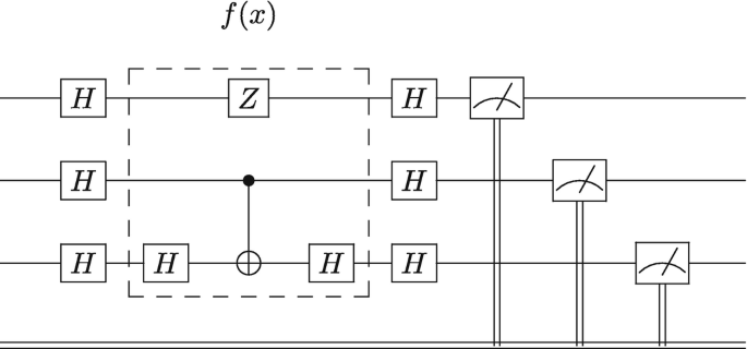

  

  The gate implementation for testing the different possible three-qubit functions.