Automatic Verification of Differential Characteristics: Application to Reduced Gimli

Abstract

Since Keccak was selected as the SHA-3 standard, more and more permutation-based primitives have been proposed. Different from block ciphers, there is no round key in the underlying permutation for permutation-based primitives. Therefore, there is a higher risk for a differential characteristic of the underlying permutation to become incompatible when considering the dependency of difference transitions over different rounds. However, in most of the MILP or SAT based models to search for differential characteristics, only the difference transitions are involved and are treated as independent in different rounds, which may cause that an invalid one is found for the underlying permutation. To overcome this obstacle, we are motivated to design a model which automatically avoids the inconsistency in the search for differential characteristics. Our technique is to involve both the difference transitions and value transitions in the constructed model. Such an idea is inspired by the algorithm to find SHA-2 characteristics as proposed by Mendel et al. in ASIACRYPT 2011, where the differential characteristic and the conforming message pair are simultaneously searched. As a first attempt, our new technique will be applied to the Gimli permutation, which was proposed in CHES 2017. As a result, we reveal that some existing differential characteristics of reduced Gimli are indeed incompatible, one of which is found in the Gimli document. In addition, since only the permutation is analyzed in the Gimli document, we are lead to carry out a comprehensive study, covering the proposed hash scheme and the authenticated encryption (AE) scheme specified for Gimli, which has become a second round candidate of the NIST lightweight cryptography standardization process. For the hash scheme, a semi-free-start (SFS) collision attack can reach up to 8 rounds starting from an intermediate round. For the AE scheme, a state recovery attack is demonstrated to achieve up to 9 rounds. It should be emphasized that our analysis does not threaten the security of Gimli.

1 Introduction

As the demand for lightweight cryptographic primitives in industry increases, NIST is currently holding a public Lightweight Cryptography Standardization process  [1], aiming at lightweight cryptography standardization by combining the efforts from both academia and industry. Among the 32 second round candidates, Gimli was first proposed in CHES 2017  [4]. The main strategy to improve its performance is to process the 384-bit data in four 96-bit columns independently and make only a 32-bit word swapping among the four columns every two rounds. Such a design strategy soon received a doubt from Hamburg  [13]. However, the attack in  [13] works for an ad-hoc mode rather than the proposed hash scheme or AE scheme in the submitted Gimli document.

Along the development of differential attacks  [7], several variants have been proposed. A very influential one was the modular differential attack on the MD-SHA hash family, which directly turned MD5  [23] and SHA-1  [20, 22] into broken hash functions. To mount collision attacks on MD5 and SHA-1 as in  [22, 23], one challenging work is to find a proper differential characteristic, which was first finished by hand-craft  [22, 23]. Later, the guess-and-determine method to search for differential characteristics was proposed in ASIACRYPT 2006, together with its application to full SHA-1  [10]. However, when such a guess-and-determine technique is directly applied to reduced SHA-2, Mendel et al. pointed out in  [18] that the discovered differential characteristics are always invalid since contradictions may easily occur in the set of conditions implied in the discovered differential characteristics. To overcome this obstacle, they finally developed an algorithm to search for the differential characteristic and the conforming message pair simultaneously to avoid the inconsistency.

Indeed, such a case does not only exist in the MD-SHA hash family. For the ARX construction, for instance, some differential characteristics of Blake-256  [8] and Skein-512  [3] are also proven to be invalid if taking some dependency into account, as revealed by Leurent  [15]. To search for valid differential characteristics of reduced Skein, Leurent designed a dedicated algorithm in  [16] using the improved generalized conditions  [15] and the guess-and-determine technique  [10].

In another direction, since the introduction of the MILP-based method to search for differential characteristics  [21], the SAT-based method has also been developed  [14]. However, in most of the MILP models or SAT models to search for differential characteristics  [4, 14, 21, 25], only the difference transitions are taken into account and are treated as independent in different rounds. Although such an assumption is commonly believed to be reasonable for block ciphers, it may not hold well for permutation-based primitives since there is no round key in the permutation. A similar problem has been investigated in  [9]. Moreover, since Keccak  [6] was selected as the SHA-3 standard, more and more permutation-based primitives have been proposed. However, whether similar cases once appearing in SHA-2  [18], Skein-512  [3] and Blake-256  [8] will occur in the commonly constructed MILP or SAT models to search for differential characteristics for the underlying permutation remains unknown. Therefore, it is vital to make an investigation for such a problem.

However, both the methods in  [16, 18] require a dedicated implementation of the heuristic search. In addition, how to achieve the simultaneousness is ambiguous in  [18]. For  [16], the inconsistency is avoided by using the improved generalized conditions  [15]. As is known, the most convincing way is to provide a conforming message pair for the discovered differential characteristic.

Therefore, similar to the motivation to introduce the MILP-based method into cryptanalysis, it would be meaningful to utilize some off-the-shelf tools to reduce the workload. Consequently, we take Gimli as our first attempt and are motivated to tackle the problem of how to construct a model to always avoid the incompatibility in the search for differential characteristics. Moreover, since Gimli is one of the second round candidates in NIST Lightweight Cryptography Standardization process, we will provide some additional analysis of reduced Gimli. We noticed that there is a related work  [19] for MD-SHA hash family published at SAT 2006 aiming at automatic message modification, though with ambiguous technical details.

Our Contributions. We made a comprehensive study of Gimli¹, as summarized below:

• We make the first step to investigate the properties of the SP-box. Such a work is meaningful since all the attacks in this paper heavily rely on them.

• A novel MILP model capturing the difference transitions and value transitions simultaneously is developed. To the best of our knowledge, this is the first model which takes both transitions into account. This model can be simply used to detect contradictions in the differential characteristic of Gimli. As a result, we prove that both the 12-round differential characteristic in the Gimli document  [4] and the 6-round differential characteristic used for the collision attack on 6-round Gimli-Hash in  [25] are invalid. The second usage of this model is to directly search for a valid differential characteristic and the conforming message pair simultaneously.

• For the hash scheme, we provide the first practical semi-free-start (SFS) colliding message pair for 6-round Gimli-Hash and develop several techniques to convert SFS collisions into collisions. Moreover, we also mount a SFS collision attack on the intermediate 8-round Gimli-Hash.

• For the AE scheme, we are curious why the designers only claim 128-bit security while a 256-bit key is used. Thus, we are motivated to devise an attack which can maximize the number of rounds with complexity below $2^{256}$. Consequently, we mount a state-recovery attack on 9-round Gimli with a rather high time complexity $2^{192}$ and memory complexity $2^{190}$.

The memory/data/time complexity of the above attacks are displayed in Table 1.

Organization. The Gimli permutation and some properties of the SP-box will be introduced in Sect. 2 and Sect. 3, respectively. Then, the MILP model capturing both difference transitions and value transitions will be described in Sect. 4. The (SFS) collision attack on 6-round and 8-round Gimli-Hash will be shown in Sect. 5 and Sect. 6, respectively. Then, we will investigate the security of the AE scheme and present the state-recovery attack on 9-round Gimli in Sect. 7. Finally, we conclude the paper in Sect. 8.

Table 1. The analytical results of reduced Gimli, where Z-S represents Zero-sum and Z-D represents Zero-internal-difference.

2 Description of Gimli

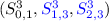
The Gimli state can be viewed as a two-dimensional array $S=(S_{i,j})$ $(0\le i\le 2, 0\le j\le 3)$, where $S_{i,j}\in F^{32}_2$, as illustrated in Fig. 1.

Fig. 1.

The Gimli state

The 24-round permutation can be viewed as iterating the following sequence of operations for 6 times:

$$\begin{aligned}&\mathrm{(SP\rightarrow S\_SW\rightarrow AC)\rightarrow (SP)\rightarrow (SP\rightarrow B\_SW)\rightarrow (SP),} \end{aligned}$$

where the SP-box operation, Small-Swap operation, Big-Swap operation and AddRoundConstant operation are denoted by SP, S_SW, B_SW and AC, respectively. For the SP-box operation, the SP-box will be applied to the four columns independently. For the AddRoundConstant operation, a 32-bit word is added to $S_{0,0}$. More details can be referred to  [4]. For convenience, denote the internal state after r-round permutation by $S^r$ and the input state by $S^0$. In other words, we have

where $0\le i\le 5$. In addition, $\varDelta S^r$ denotes the exclusive or difference in $S^r$ ($0\le r\le 24$). Z[i] $(0\le i\le 31)$ denotes the $(i+1)$-th bit of the 32-bit word Z and Z[0] is the least significant bit of Z. $Z[i\sim j] (0\le j<i\le 31)$ represents the $(j+1)$-th bit to the $(i+1)$-th bit of the 32-bit word Z. For example, $Z[1\sim 0]$ represents the two bits (Z[1],Z[0]). Moreover, $\oplus$, $\ll$, $\lll$, $\vee$ and $\wedge$ represent the logic operations exclusive or, shift left, rotate left, or, and, respectively.

2.1 SP-box

The SP-box of Gimli takes a 96-bit value as input and outputs a 96-bit value. Denote the input and the output by $(IX,IY,IZ)\in F_2^{32\times 3}$ and $(OX,OY,OZ)\in F_2^{32\times 3}$, respectively. Then, the relation between (OX, OY, OZ) and (IX, IY, IZ) can be described as follows:

$$\begin{aligned} IX\leftarrow & {} IX\lll 24\\ IY\leftarrow & {} IY\lll 9\\ OZ\leftarrow & {} IX\oplus IZ\ll 1 \oplus (IY\wedge IZ)\ll 2\\ OY\leftarrow & {} IY\oplus IX \oplus (IX\vee IZ)\ll 1\\ OX\leftarrow & {} IZ\oplus IY \oplus (IX\wedge IY)\ll 3 \end{aligned}$$

Based on the above relation, the following bit relations can be derived, where the indices are considered within modulo 32.

$$\begin{aligned} OX[i]= \left\{ \begin{aligned}&IZ[i]\oplus IY[i-9] \ (0\le i\le 2)\\&IZ[i]\oplus IY[i-9] \oplus (IX[i-27]\wedge IY[i-12]) \ (3\le i\le 31) \end{aligned} \right. \end{aligned}$$

(1)

$$\begin{aligned} OY[i]= \left\{ \begin{aligned}&IY[i-9]\oplus IX[i-24] \ (i=0)\\&IY[i-9]\oplus IX[i-24]\oplus (IX[i-25]\vee IZ[i-1]) \ (1\le i\le 31) \end{aligned} \right. \end{aligned}$$

(2)

$$\begin{aligned} OZ[i]= \left\{ \begin{aligned}&IX[i-24] \ (i=0)\\&IX[i-24]\oplus IZ[i-1] \ (i=1)\\&IX[i-24]\oplus IZ[i-1]\oplus (IY[i-11]\wedge IZ[i-2]) \ (2\le i\le 31) \end{aligned} \right. \end{aligned}$$

(3)

2.2 Linear Layer

The linear layer includes two different swap operations, namely Small-Swap and Big-Swap. Small-Swap occurs every 4 rounds starting from the 1st round. Big-Swap occurs every 4 rounds starting from the 3rd round. The illustration of Small-Swap and Big-Swap can be referred to Fig. 2.

Fig. 2.

The linear layer. The left/right one represent the Small-Swap/Big-Swap.

2.3 Gimli-Hash

How Gimli-Hash compresses a message is illustrated in Fig. 3. Specifically, Gimli-Hash initializes a 48-byte Gimli state to all-zero. It then reads sequentially through a variable-length input as a series of 16-byte input blocks, denoted by $M_0$, $M_1$, $\cdot \cdot \cdot$. After all message blocks are processed, the 256-bit hash value will be generated. More details can be referred to  [1].

Fig. 3.

The process to compress the message, where f is the Gimli permutation

3 Properties of the SP-box

Since several properties of the SP-box will be exploited in our collision attack and state-recovery attack, for convenience, we summarize them in this part. For simplicity, the input and output of the SP-box are denoted by (IX, IY, IZ) and (OX, OY, OZ), respectively.

Property 1

If $IY[31\sim 23]=0$ and $IY[19\sim 0]=0$, OX will be independent of IX.

Property 2

A random triple (IY, IZ, OX) is potentially valid with probability $2^{-15.5}$ without knowing IX.

Property 3

Given a random triple (IX, OY, OZ), it is valid with probability $2^{-1}$. Once it is valid, $(OX[30\sim 0],IY,IZ[30\sim 0])$ can be determined.

Property 4

Given a random triple (IY, IZ, OZ), (IX, OX, OY) can be uniquely determined. In addition, a random tuple (IY, IZ, OY, OZ) is valid with probability $2^{-32}$.

Property 5

Suppose the pair (IY, IZ) and t bits of OY are known. Then t bits of information on IX can be recovered by solving a linear equation system of size t.

The above properties will be frequently exploited in our attacks and therefore we list them ahead of time. The corresponding proofs can be referred to the full version of this paper  [17]. Some other properties will be explained later.

4 The MILP Model Capturing Difference and Value Transitions

To search for a valid differential characteristic of reduced SHA-2, Mendel et al. developed a technique to search for the differential characteristic and conforming message pair simultaneously  [18]. However, how to achieve the simultaneousness is not explained in  [18]. Inspired by such an idea, different from many models where only the difference transitions are considered and are treated as independent in different rounds, we try to construct a model which can describe the difference transitions and value transitions simultaneously. The basic idea is simple. As shown in Fig. 4, the models to describe the difference transitions and value transitions will be independently constructed. Then, construct a model to describe the difference-value relations in the nonlinear operation and use it to connect the difference transitions and value transitions. The reason is that the difference transitions and value transitions are dependent only in the nonlinear operation. If such a model can be constructed, the contradictions can always be avoided in the search.

Fig. 4.

Illustration of the model

4.1 Difference-Value Relations Through the SP-box

First of all, consider the relations between the difference and value. According to the bit relations between (IX, IY, IZ) and (OX, OY, OZ) as specified in Eq. 1, Eq. 2, and Eq. 3, one can easily observe that there are at most 4 types of Boolean expressions as follows, where $a[i]\in F_2$ and $0\le i\le 4$.

• Type-1: $a[1]=a[0]$.

• Type-2: $a[2]=a[0]\oplus a[1]$.

• Type-3: $a[4]=a[0]\oplus a[1]\oplus a[2]\wedge a[3]$.

• Type-4: $a[4]=a[0]\oplus a[1]\oplus a[2]\vee a[3]$.

Specifically, Type-1 corresponds to the expression to calculate OZ[0]. Type-2 corresponds to the expressions to calculate OX[0], OX[1], OX[2], OY[0] and OZ[1]. Type-3 corresponds to the expression to compute OX[i] $(3\le i\le 31)$ and OZ[j] $(2\le j\le 31)$, while Type-4 corresponds to the expression to compute OY[i] $(1\le i\le 31)$.

For convenience, introduce another 5 bit variables $a^{\prime }$ = {$a^{\prime }[0]$, $a^{\prime }[1]$, $a^{\prime }[2]$, $a^{\prime }[3]$, $a^{\prime }[4]$} and let $\varDelta a=a\oplus a^{\prime }$, i.e. $\varDelta a[i]=a[i]\oplus a^{\prime }[i]$ for $0\le i\le 4$. For better understanding, we explain the relations between the difference $(\varDelta a)$ and the value (a) for each of the 4 types.

Type-1. For this type, there is no relation between $\varDelta a$ and a. Only the following relation can be derived:

$$\begin{aligned} \varDelta a[1]=\varDelta a[0]. \end{aligned}$$

Type-2. Similar to Type-1, there is no relation between $\varDelta a$ and a. Only the following relation can be derived:

$$\begin{aligned} \varDelta a[2]=\varDelta a[0] \oplus \varDelta a[1]. \end{aligned}$$

Type-3. Since a nonlinear operation exists in this expression, we can derive the relations between $\varDelta a$ and a, as specified below:

$$\begin{aligned}&\varDelta a[4]\oplus \varDelta a[0] \oplus \varDelta a[1] =1, \varDelta a[2]=0, \varDelta a[3]=0\Rightarrow Contradiction\\&\varDelta a[4]\oplus \varDelta a[0] \oplus \varDelta a[1] =1, \varDelta a[2]=0, \varDelta a[3]=1\Rightarrow a[2]=1\\&\varDelta a[4]\oplus \varDelta a[0] \oplus \varDelta a[1] =1, \varDelta a[2]=1, \varDelta a[3]=0\Rightarrow a[3]=1\\&\varDelta a[4]\oplus \varDelta a[0] \oplus \varDelta a[1] =1, \varDelta a[2]=1, \varDelta a[3]=1\Rightarrow a[2]=a[3]\\&\varDelta a[4]\oplus \varDelta a[0] \oplus \varDelta a[1] =0, \varDelta a[2]=0, \varDelta a[3]=1\Rightarrow a[2]=0\\&\varDelta a[4]\oplus \varDelta a[0] \oplus \varDelta a[1] =0, \varDelta a[2]=1, \varDelta a[3]=0\Rightarrow a[3]=0\\&\varDelta a[4]\oplus \varDelta a[0] \oplus \varDelta a[1] =0, \varDelta a[2]=1, \varDelta a[3]=1\Rightarrow a[2]\oplus a[3]=1. \end{aligned}$$

Type-4. Similar to Type-3, since a nonlinear operation exists in this expression, the following relations between $\varDelta a$ and a can be derived:

$$\begin{aligned}&\varDelta a[4]\oplus \varDelta a[0] \oplus \varDelta a[1] =1, \varDelta a[2]=0, \varDelta a[3]=0\Rightarrow Contradiction\\&\varDelta a[4]\oplus \varDelta a[0] \oplus \varDelta a[1] =1, \varDelta a[2]=0, \varDelta a[3]=1\Rightarrow a[2]=0\\&\varDelta a[4]\oplus \varDelta a[0] \oplus \varDelta a[1] =1, \varDelta a[2]=1, \varDelta a[3]=0\Rightarrow a[3]=0\\&\varDelta a[4]\oplus \varDelta a[0] \oplus \varDelta a[1] =1, \varDelta a[2]=1, \varDelta a[3]=1\Rightarrow a[2]=a[3]\\&\varDelta a[4]\oplus \varDelta a[0] \oplus \varDelta a[1] =0, \varDelta a[2]=0, \varDelta a[3]=1\Rightarrow a[2]=1\\&\varDelta a[4]\oplus \varDelta a[0] \oplus \varDelta a[1] =0, \varDelta a[2]=1, \varDelta a[3]=0\Rightarrow a[3]=1\\&\varDelta a[4]\oplus \varDelta a[0] \oplus \varDelta a[1] =0, \varDelta a[2]=1, \varDelta a[3]=1\Rightarrow a[2]\oplus a[3]=1. \end{aligned}$$

4.2 Constructing the MILP Model

It has been discussed above that there are only two cases when we need to consider the relations between the difference and value transitions through the SP-box. Thus, we first construct the MILP model to describe such relations. First of all, consider two minimal models called AND-Model and OR-Model.

Constructing AND-Model. Consider the following Boolean expression

$$\begin{aligned} a[2]=a[0]\wedge a[1]. \end{aligned}$$

Firstly, construct the truth table for $(a[0],a[1],\varDelta a[0], \varDelta a[1], \varDelta a[2])$, which can be easily finished by enumerating all 16 possible values of $(a[0],a[1],\varDelta a[0], \varDelta a[1])$ and computing the corresponding $\varDelta a[2]$. Details are given in the full version of this paper  [17]. Using the greedy algorithm in  [21], the corresponding truth table can be described with the following linear inequalities, where the remaining 16 invalid patterns can not satisfy at least one of them.

$$\begin{aligned} \left\{ \begin{aligned} -a[0] - a[1] - \varDelta a[1] + \varDelta a[2]+2&\ge 0\\ a[0] - a[1] - \varDelta a[1] - \varDelta a[2]+2&\ge 0\\ -a[0] + a[1] - \varDelta a[0] - \varDelta a[2]+2&\ge 0\\ a[0] + \varDelta a[0] - \varDelta a[2]&\ge 0\\ a[0] + a[1] - \varDelta a[0] - \varDelta a[1] + \varDelta a[2]+1&\ge 0\\ \varDelta a[0] + \varDelta a[1] - \varDelta a[2]&\ge 0\\ a[1] + \varDelta a[1] - \varDelta a[2]&\ge 0\\ - a[1] - \varDelta a[0] + \varDelta a[1] + \varDelta a[2]+1&\ge 0\\ -a[0] + \varDelta a[0] - \varDelta a[1] + \varDelta a[2]+1&\ge 0 \end{aligned} \right. \end{aligned}$$

(4)

Constructing OR-Model. Consider the following Boolean expression

$$\begin{aligned} a[2]=a[0]\vee a[1]. \end{aligned}$$

Similarly, construct the truth table for $(a[0],a[1],\varDelta a[0], \varDelta a[1], \varDelta a[2])$ by enumerating all 16 possible values of $(a[0],a[1],\varDelta a[0], \varDelta a[1])$ and computing the corresponding $\varDelta a[2]$. Details are given in the full version of this paper  [17]. The corresponding truth table is equivalent to the following linear inequalities:

$$\begin{aligned} \left\{ \begin{aligned} - a[1] + \varDelta a[1] - \varDelta a[2] + 1&\ge 0\\ -a[0] + \varDelta a[0] - \varDelta a[2] + 1&\ge 0\\ a[1] - \varDelta a[0] + \varDelta a[1] + \varDelta a[2]&\ge 0\\ a[0] + \varDelta a[0] - \varDelta a[1] + \varDelta a[2]&\ge 0\\ a[0] + a[1] - \varDelta a[1] + \varDelta a[2]&\ge 0\\ \varDelta a[0] + \varDelta a[1] - \varDelta a[2]&\ge 0\\ a[0] - a[1] - \varDelta a[0] - \varDelta a[2] + 2&\ge 0\\ -a[0] - a[1] - \varDelta a[0] - \varDelta a[1] + \varDelta a[2] + 3&\ge 0\\ -a[0] + a[1] - \varDelta a[1] - \varDelta a[2] + 2&\ge 0 \end{aligned} \right. \end{aligned}$$

(5)

Constructing MILP Model for Value Transitions. For the Gimli round function, the linear layer can be viewed as a simple permutation of bit positions. Thus, we only focus on the model to describe the value transitions through the SP-box in this part. As discussed above, there are at most 4 types of Boolean expressions when expressing the output bit in terms of the input bits for the SP-box. Now, we explain how to model such 4 types of expressions.

Modeling Type-1 Expression. The Type-1 Boolean expression is

$$\begin{aligned} a[1]=a[0]. \end{aligned}$$

Thus, it is rather simple to model the value relation by using the following linear equality:

$$\begin{aligned} a[1]=a[0]. \end{aligned}$$

(6)

Modeling Type-2 Expression. The Type-2 Boolean expression is

$$\begin{aligned} a[2]=a[0]\oplus a[1]. \end{aligned}$$

Such a linear Boolean equation can be described with the following linear inequalities:

$$\begin{aligned} \left\{ \begin{aligned} a[0]+a[1]-a[2]&\ge 0\\ a[0]-a[1]+a[2]&\ge 0\\ -a[0]+a[1]+a[2]&\ge 0\\ -a[0]-a[1]-a[2]+2&\ge 0 \end{aligned} \right. \end{aligned}$$

(7)

Modeling Type-3 Expression. The Type-3 Boolean expression is

$$\begin{aligned} a[4]=a[0]\oplus a[1]\oplus a[2]\wedge a[3]. \end{aligned}$$

Such a linear Boolean equation can be described with the following linear inequalities:

$$\begin{aligned} \left\{ \begin{aligned} -a[0] + a[1] + a[3] + a[4]&\ge 0\\ a[0] - a[1] + a[3] + a[4]&\ge 0\\ a[0] + a[1] + a[2] - a[4]&\ge 0\\ a[0] + a[1] + a[3] - a[4]&\ge 0\\ a[0] - a[1] + a[2] + a[4]&\ge 0\\ -a[0] + a[1] + a[2] + a[4]&\ge 0\\ a[0] + a[1] - a[2] - a[3] + a[4] + 1&\ge 0\\ -a[0] - a[1] + a[2] - a[4] + 2&\ge 0\\ a[0] - a[1] - a[2] - a[3] - a[4] + 3&\ge 0\\ -a[0] - a[1] - a[2] - a[3] + a[4] + 3&\ge 0\\ -a[0] - a[1] + a[3] - a[4] + 2&\ge 0\\ -a[0] + a[1] - a[2] - a[3] - a[4] + 3&\ge 0 \end{aligned} \right. \end{aligned}$$

(8)

Modeling Type-4 Expression. The Type-4 Boolean expression is

$$\begin{aligned} a[4]=a[0]\oplus a[1]\oplus a[2]\vee a[3]. \end{aligned}$$

Such a linear Boolean equation can be described with the following linear inequalities:

$$\begin{aligned} \left\{ \begin{aligned} -a[0] + a[1] - a[3] - a[4] + 2&\ge 0\\ a[0] - a[1] - a[3] - a[4] + 2&\ge 0\\ -a[0] - a[1] - a[3] + a[4] + 2&\ge 0\\ -a[0] + a[1] - a[2] - a[4] + 2&\ge 0\\ a[0] - a[1] - a[2] - a[4] + 2&\ge 0\\ -a[0] - a[1] - a[2] + a[4] + 2&\ge 0\\ -a[0] + a[1] + a[2] + a[3] + a[4]&\ge 0\\ a[0] + a[1] - a[3] + a[4]&\ge 0\\ a[0] + a[1] - a[2] + a[4]&\ge 0\\ a[0] - a[1] + a[2] + a[3] + a[4]&\ge 0\\ a[0] + a[1] + a[2] + a[3] - a[4]&\ge 0\\ -a[0] - a[1] + a[2] + a[3] - a[4] + 2&\ge 0 \end{aligned} \right. \end{aligned}$$

(9)

Constructing MILP Model for Difference Transitions. The value transitions through the SP-box have been discussed above. In the following, how to model the difference transitions will be detailed. Similarly, write the four possible types of expressions for differences as follows:

$$\begin{aligned}&\varDelta a[1]=\varDelta a[0], \end{aligned}$$

(10)

$$\begin{aligned}&\varDelta a[2]=\varDelta a[0]\oplus \varDelta a[1], \end{aligned}$$

(11)

$$\begin{aligned}&\varDelta a[4]=\varDelta a[0]\oplus \varDelta a[1] \oplus \varDelta na_0,\end{aligned}$$

(12)

$$\begin{aligned}&\varDelta a[4]=\varDelta a[0]\oplus \varDelta a[1] \oplus \varDelta na_1, \end{aligned}$$

(13)

where $na_0$ and $na_1$ represent the output difference of the nonlinear operation $a[2]\wedge a[3]$ and $a[2]\vee a[3]$, respectively. It can be easily observed that the first two possible transitions (Eq. 10 and Eq. 11) share the same MILP model used to describe the value transitions for Type-1 expression and Type-2 expression. For the last two transitions, we need to construct a model to describe the following linear Boolean equation:

$$\begin{aligned} a[3]=a[0]\oplus a[1]\oplus a[2]. \end{aligned}$$

This task is also rather easy. The linear inequalities to describe the above linear Boolean equation in terms of four variables are specified as follows:

$$\begin{aligned} \left\{ \begin{aligned} a[0] + a[1] - a[2] + a[3]&\ge 0\\ a[0] + a[1] + a[2] - a[3]&\ge 0\\ -a[0] + a[1] + a[2] + a[3]&\ge 0\\ a[0] - a[1] + a[2] + a[3]&\ge 0\\ -a[0] - a[1] + a[2] - a[3] + 2&\ge 0\\ a[0] - a[1] - a[2] - a[3] + 2&\ge 0\\ -a[0] + a[1] - a[2] - a[3] + 2&\ge 0\\ -a[0] - a[1] - a[2] + a[3] + 2&\ge 0\\ \end{aligned} \right. \end{aligned}$$

(14)

One may observe that two intermediate variables $na_0$ and $na_1$ are introduced when constructing the model for difference transitions and they have not been connected with the actual variables, i.e. a and $\varDelta a$ in the constructed model. In fact, this is where our technique exists in order to model the difference and value transitions simultaneously. Specifically, the two intermediate variables $na_0$ and $na_1$ will be utilized to link the value transitions and difference transitions, together with the two minimal models AND-Model and OR-Model.

Connecting the Value Transitions and Difference Transitions. It can be observed that the current MILP models for value transitions and difference transitions are independently constructed. In this part, we will describe how to connect the value and difference transitions with the two intermediate variables ($na_0$, $na_1$) by using the AND-Model and OR-Model. Note that $na_0$ and $na_1$ denote the output difference of the nonlinear operations $a[2]\wedge a[3]$ and $a[2]\vee a[3]$, respectively.

Connecting the Two Transitions for Type-3 Expression. Consider the Type-3 expression:

$$\begin{aligned} a[4]=a[0]\oplus a[1]\oplus a[2]\wedge a[3]. \end{aligned}$$

Firstly, use Eq. 8 to model the relations of (a[0], a[1], a[2], a[3], a[4]). Then, use the AND-Model to describe the relations of $(a[2],a[3],\varDelta a[2],\varDelta a[3],na_0)$. Finally, use Eq. 14 to describe the relations of $(\varDelta a[0],\varDelta a[1], na_0,\varDelta a[4])$. In this way, the value and difference transitions for Type-3 expression are connected.

Connecting the Two Transitions for Type-4 Expression. The Type-4 expression is specified as follows:

$$\begin{aligned} a[4]=a[0]\oplus a[1]\oplus a[2]\vee a[3]. \end{aligned}$$

Similarly, Eq. 9 is used to model the relations of (a[0], a[1], a[2], a[3], a[4]). Then, the OR-Model is used to model the relations of $(a[2],a[3],\varDelta a[2],\varDelta a[3],na_1)$. At last, Eq. 14 is used to describe the relations of $(\varDelta a[0],\varDelta a[1], na_1,\varDelta a[4])$.

For the remaining two expressions (Type-1 and Type-2), the value and difference transitions are independent. Therefore, the corresponding two models are independent and there is no need to connect them. Obviously, the AND-Model and OR-Model are the core techniques to achieve the connection.

4.3 Detecting Contradictions

Since both the difference transitions and value transitions are taken into account in our MILP model, once given a specified differential characteristic of Gimli, the difference transitions are fixed. In addition, some constraints on the value of the internal states are fixed as well based on the AND-Model and OR-Model. Thus, the final inequality system in the whole model is only in terms of the variables representing the value of the internal states. If a solution can be returned by the solver, it simply means that there is a conforming message pair satisfying the differential characteristic. However, if the solver returns “infeasible”, it implies that no conforming message pair can satisfy the differential characteristic, thus revealing that the differential characteristic is impossible.

We have used the above method to check the validity of two existing differential characteristics of Gimli. One is the 12-round differential characteristic proposed in the Gimli document  [4], and the other is the 6-round differential characteristic used for a collision attack in  [25]. Surprisingly, both of them are proven to be invalid, i.e. the Gurobi solver  [2] returns “infeasible”. To support the correctness of our model, detailed analysis of the contradictions are provided in the full version of this paper  [17].

5 Collision Attack on 6-Round Gimli-Hash

Since the 6-round differential characteristic is invalid in  [25], it is necessary to search for a valid one in order to mount a collision attack on 6-round Gimli-Hash. On the whole, our collision attack procedure can be divided into the following two phases:

Phase 1::

Utilize our model to find a valid 6-round differential characteristic.

Phase 2::

Use the linearization and start-from-the-middle techniques to find all the conforming message pairs satisfying the discovered differential characteristic and store them in a clever way. All these message pairs can be viewed as SFS colliding message pairs. Then, convert the SFS collisions into collisions with a divide-and-conquer method.

Obviously, both the way to search for a differential characteristic and the way to mount a collision attack are different from that in  [25].

5.1 Searching a Valid 6-Round Differential Characteristic

It can be easily observed in  [25] that, in order to eliminate the influence of linear layer (Big-Swap and Small-Swap) and to reduce the workload of the MILP model, the authors only considered the difference transitions in one column rather than the whole state. Specifically, as shown in Fig. 5, the target is to find the following valid difference transitions through the SP-box:

Once such a solution is found, it can be easily converted into a differential characteristic of the full state. However, as has been proved, the solution found in  [25] is actually invalid if considering the dependency between the value transitions and difference transitions.

Fig. 5.

The pattern of the difference transitions in  [25]

Different from the optimal differential characteristic which may be sparse, the differential characteristic used for the collision attack is much denser, thus having a high probability that contradictions occur if only the difference transitions are considered. To avoid such a bad case, the differential characteristic and the conforming message pair will be simultaneously searched with our constructed MILP model. Similar to  [4, 25], a probability 1 two-round differential characteristic is first constructed in the last two rounds. Moreover, to reduce the workload, some additional constraints will be added when constructing the model, as specified below:

$$\begin{aligned}&\varDelta S^0_{i,0}=\varDelta S^0_{i,2}=0 \ (0 \le i\le 2). \end{aligned}$$

(15)

$$\begin{aligned}&\varDelta S^0_{j,1}=\varDelta S^0_{j,3}=0 \ (1 \le j\le 2).\end{aligned}$$

(16)

$$\begin{aligned}&\varDelta S^4_{i,0}=\varDelta S^4_{i,2}=0 \ (0 \le i\le 2).\end{aligned}$$

(17)

$$\begin{aligned}&\varDelta S^4_{j,1}=\varDelta S^4_{j,3}=0 \ (1 \le j\le 2).\end{aligned}$$

(18)

$$\begin{aligned}&\varDelta S^r_{i,j}=\varDelta S^r_{i,j+2}\ (0 \le i\le 2, 0\le j\le 1, 0\le r\le 3).\end{aligned}$$

(19)

$$\begin{aligned}&\varDelta S^4_{0,1}=\varDelta S^4_{0,3}=\texttt {0x80}.\end{aligned}$$

(20)

$$\begin{aligned}&\varDelta S^4_{1,1}=\varDelta S^4_{1,3}=\texttt {0x400000}.\end{aligned}$$

(21)

$$\begin{aligned}&\varDelta S^4_{2,1}=\varDelta S^4_{2,3}=\texttt {0x80000000}. \end{aligned}$$

(22)

Moreover, to reduce the search space, we further constrain the hamming weight of $(\varDelta S^3_{0,1},\varDelta S^3_{1,1},\varDelta S^3_{2,1})$ as follows, i.e. the number of bits whose values are 1:

$$\begin{aligned} HW(\varDelta S^3_{0,1},\varDelta S^3_{1,1},\varDelta S^3_{2,1})\le 8. \end{aligned}$$

Specifically, the aim is to find a solution for the 32-bit words marked with “?” in Fig. 6.

Fig. 6.

Searching a valid 6-round differential characteristic

The 6-Round Differential Characteristic. Based on the above model, the Gurobi solver returns a solution in less than 4 h. In other words, a valid 6-round differential characteristic and a conforming message pair are obtained. For a better presentation, the differential characteristic is displayed in Table 2. The conforming message pair is displayed in Table 4. The conditions implied in the differential characteristic are shown in Table 3. Note that by using one more message block to eliminate the difference in the rate part, a full-state SFS collision is obtained. However, the SFS collision attack is still less meaningful than the collision attack. Therefore, we are further motivated to convert the SFS collisions into collisions.

Table 2. The 6-round differential characteristic

Table 3. The conditions implied in the 6-round differential characteristic

Table 4. The conforming message pair for the 6-round differential characteristic

5.2 Converting SFS Collision Attacks into Collision Attacks

First of all, as shown in Table 3, the conditions on $S^3_{0,1}$ and $S^3_{0,3}$ only involve the bits of $S^3_{0,1}$ and $S^3_{0,3}$, respectively. Due to the symmetry of the 6-round differential characteristic, the conditions on $S^3_{0,1}$ and $S^3_{0,3}$ are the same. Due to the influence of Big-Swap, $S^3_{0,3}$ is actually computed by using $(S^2_{0,1},S^2_{1,1},S^2_{2,1})$, while $S^3_{0,1}$ is computed by using $(S^2_{0,3},S^2_{1,3},S^2_{2,3})$. Thus, we define two sets of conditions which can be independently verified, as specified below:

Definition 1

The internal state words $(S^0_{0,1},S^0_{1,1},S^0_{2,1})$, $(S^1_{0,1},S^1_{1,1},S^1_{2,1})$, $(S^2_{0,1},S^2_{1,1},S^2_{2,1})$ and only depend on the input state words $(S^0_{i,j})$ $(0\le i\le 2, 0\le j\le 1)$, while the internal state words $(S^0_{0,3},S^0_{1,3},S^0_{2,3})$, $(S^1_{0,3},S^1_{1,3},S^1_{2,3})$, $(S^2_{0,3},S^2_{1,3},S^2_{2,3})$ and only depend on the input state words $(S^0_{i,j})$ $(0\le i\le 2, 2\le j\le 3)$.

Therefore, by only knowing $(S^0_{i,j})$ $(0\le i\le 2, 0\le j\le 1)$, we can fully compute $(S^0_{0,1},S^0_{1,1},S^0_{2,1})$, $(S^1_{0,1},S^1_{1,1},S^1_{2,1})$, $(S^2_{0,1},S^2_{1,1},S^2_{2,1})$ and . For simplicity, the conditions on these 12 internal state words in Table 3 are called $\mathbf{L}-Conditions$.

Similarly, by only knowing $(S^0_{i,j})$ $(0\le i\le 2, 2\le j\le 3)$, we can fully compute $(S^0_{0,3},S^0_{1,3},S^0_{2,3})$, $(S^1_{0,3},S^1_{1,3},S^1_{2,3})$, $(S^2_{0,3},S^2_{1,3},S^2_{2,3})$ and . For simplicity, the conditions on these 12 internal state words in Table 3 are called $\mathbf{R}-Conditions$.

Therefore, the L-Conditions and R-Conditions can be verified independently. Now, we introduce a method to identify all the possible values for the capacity of the first two columns $(S^0_{i,j})$ $(1\le i\le 2, 0\le j\le 1)$ which can fulfill the L-Conditions. Since the L-Conditions and R-Conditions are identical, the method works in the same way to find all the possible values for the capacity part of the last two columns $(S^0_{i,j})$ $(1\le i\le 2, 2\le j\le 3)$ which can fulfill the R-Conditions.

Identifying All Possible Solutions. To obtain all valid values of $(S^0_{i,j})$ $(1\le i\le 2, 0\le j\le 1)$, the following techniques will be exploited to accelerate the exhaustive search:

• 1. Merge the conditions in two consecutive rounds, which can significantly reduce the size of the search space.

• 2. Use a start-from-the-middle method and the properties of the SP-box to further accelerate the exhaustive search.

Instead of directly finding all valid values for $(S^0_{i,j})$ $(1\le i\le 2, 0\le j\le 1)$, we will first search for all the valid solutions for $(S^1_{0,1},S^1_{1,1},S^1_{2,1})$. It should be noted that once $(S^1_{0,1},S^1_{1,1},S^1_{2,1})$ are known, $(S^2_{0,1},S^2_{1,1},S^2_{2,1})$ and can be fully determined. In other words, we can first identify all the solutions for $(S^1_{0,1},S^1_{1,1},S^1_{2,1})$ which can make the conditions on $(S^1_{0,1},S^1_{1,1},S^1_{2,1})$, $(S^2_{0,1},S^2_{1,1},S^2_{2,1})$ and hold.

Merging the Conditions. According to Table 3, there are 40 linearly independent conditions on $(S^1_{0,1},S^1_{1,1},S^1_{2,1})$. Moreover, there are 41 linearly independent conditions on $(S^2_{0,1},S^2_{1,1},S^2_{2,1})$. The basic idea to convert partial conditions on $(S^2_{0,1},S^2_{1,1},S^2_{2,1})$ into those on $(S^1_{0,1},S^1_{1,1},S^1_{2,1})$ is simple. Specifically, represent the conditions on $(S^1_{0,1},S^1_{1,1},S^1_{2,1})$ using a matrix $LM_1$ at first. Then, represent the conditions on $(S^2_{0,1},S^2_{1,1},S^2_{2,1})$ using another matrix $LM_2$. Consider the following relations between $(S^1_{0,1},S^1_{1,1},S^1_{2,1})$ and $(S^2_{0,1},S^2_{1,1},S^2_{2,1})$:

$$\begin{aligned} S^2_{0,1}[i]= \left\{ \begin{aligned}&S^1_{2,1}[i]\oplus S^1_{1,1}[i-9] \ (0\le i\le 2)\\&S^1_{2,1}[i]\oplus S^1_{1,1}[i-9] \oplus (S^1_{0,1}[i-27]\wedge S^1_{1,1}[i-12]) \ (3\le i\le 31) \end{aligned} \right. \end{aligned}$$

$$\begin{aligned} S^2_{1,1}[i]= \left\{ \begin{aligned}&S^1_{1,1}[i-9]\oplus S^1_{0,1}[i-24] \ (i=0)\\&S^1_{1,1}[i-9]\oplus S^1_{0,1}[i-24]\oplus (S^1_{0,1}[i-25]\vee S^1_{2,1}[i-1]) \ (1\le i\le 31) \end{aligned} \right. \end{aligned}$$

$$\begin{aligned} S^2_{2,1}[i]= \left\{ \begin{aligned}&S^1_{0,1}[i-24] \ (i=0)\\&S^1_{0,1}[i-24]\oplus S^1_{2,1}[i-1] \ (i=1)\\&S^1_{0,1}[i-24]\oplus S^1_{2,1}[i-1]\oplus (S^1_{1,1}[i-11]\wedge S^1_{2,1}[i-2]) \ (2\le i\le 31) \end{aligned} \right. \end{aligned}$$

Therefore, if there are conditions on $S^2_{0,1}[i]$ $(0\le i\le 2)$ or on $S^2_{1,1}[0]$ or on $S^2_{2,1}[i]$ $(0\le i\le 1)$, they can be directly converted into linear conditions on $(S^1_{0,1},S^1_{1,1},S^1_{2,1})$. Thus, we can add these newly-generated conditions to $LM_1$ and apply the Gauss elimination. As for the remaining conditions on $(S^2_{0,1},S^2_{1,1},S^2_{2,1})$, we first check whether the nonlinear part $S^1_{0,1}[i-27]\,\wedge \, S^1_{1,1}[i-12]$ or $S^1_{0,1}[i-25]\vee S^1_{2,1}[i-1]$ or $S^1_{1,1}[i-11]\wedge S^1_{2,1}[i-2]$ can be linearized based on the conditions on $(S^1_{0,1},S^1_{1,1},S^1_{2,1})$. Specifically, if one bit of the nonlinear part is fixed in $(S^1_{0,1},S^1_{1,1},S^1_{2,1})$, the corresponding conditions on $(S^2_{0,1},S^2_{1,1},S^2_{2,1})$ can be directly converted into linear conditions on $(S^1_{0,1},S^1_{1,1},S^1_{2,1})$. Then, we add these newly-generated linear conditions to $LM_1$ and again apply the Gauss elimination. Such a process is repeated until $LM_1$ becomes stable, i.e. no more conditions on $(S^2_{0,1},S^2_{1,1},S^2_{2,1})$ can be converted into new linear conditions on $(S^1_{0,1},S^1_{1,1},S^1_{2,1})$. In this way, there will be finally 61 linearly independent conditions on $(S^1_{0,1},S^1_{1,1},S^1_{2,1})$. In other words, the size of the solution space of $(S^1_{0,1},S^1_{1,1},S^1_{2,1})$ is reduced to $2^{96-61}=2^{35}$ from $2^{96-40}=2^{56}$ after converting partial conditions on $(S^2_{0,1},S^2_{1,1},S^2_{2,1})$ into those on $(S^1_{0,1},S^1_{1,1},S^1_{2,1})$.

The Start-From-the-Middle Method. According to the above analysis, the solution space of $(S^1_{0,1},S^1_{1,1},S^1_{2,1})$ can now be exhausted in practical time $2^{35}$. For each of its possible values, the conditions on $(S^2_{0,1},S^2_{1,1},S^2_{2,1})$ and can be fully verified. In this way, we find that there are in total 1632 solutions for $(S^1_{0,1},S^1_{1,1},S^1_{2,1})$. By sorting the solutions according to $(S^1_{1,1},S^1_{2,1})$, we find that among all the 1632 solutions, there are 720 different values of $(S^1_{1,1},S^1_{2,1})$ and each different value of $(S^1_{1,1},S^1_{2,1})$ will correspond to 2 different values of $S^1_{0,1}$ on average. Record these 720 different values of $(S^1_{1,1},S^1_{2,1})$ in order to identify all the valid values of $(S^0_{1,1},S^0_{2,1})$.

It has been discussed in Property 4 that a random tuple $(S^0_{1,1},S^0_{2,1},S^1_{1,1},S^1_{2,1})$ is valid with probability $2^{-32}$. Once it is valid, $(S^0_{0,1},S^1_{0,1})$ is determined. In other words, although the attacker can freely choose the values of $S^0_{0,1}$, whether the 720 different values of $(S^1_{1,1},S^1_{2,1})$ can be reached only depends on the value of $(S^0_{1,1},S^0_{2,1})$. According to Table 3, there are 27 linearly independent conditions on $(S^0_{1,1},S^0_{2,1})$. Thus, a naive way to find all the valid solutions of $(S^0_{1,1},S^0_{2,1})$ is to exhaust all the $2^{64-27}=2^{37}$ possible values of $(S^0_{1,1},S^0_{2,1})$ since we can pre-assign values to $(S^0_{1,1},S^0_{2,1})$ to make the 27 linear conditions on them hold. For each guessed value, check whether there exists a tuple $(S^1_{1,1},S^1_{2,1})$ which can make the tuple $(S^0_{1,1},S^0_{2,1},S^1_{1,1},S^1_{2,1})$ valid. Obviously, the time complexity of this method is $720\times 2^{37}=2^{46.4}$ and therefore it still requires a significant amount of time. To accelerate this exhaustive search, we use the following property of the SP-box.

Property 6

Given the triple (IZ, OY, OZ), IY can be recovered by solving a linear equation system of size 32.

Proof

For simplicity, we omit the rotate shift of (IX, IY) and only focus on the following relations.

$$\begin{aligned} OZ\leftarrow & {} IX\oplus IZ\ll 1 \oplus (IY\wedge IZ)\ll 2\\ OY\leftarrow & {} IY\oplus IX \oplus (IX\vee IZ)\ll 1\\ OX\leftarrow & {} IZ\oplus IY \oplus (IX\wedge IY)\ll 3 \end{aligned}$$

Therefore, we can obtain that

Since (IZ, OY, OZ) are known, 32 linearly independent equations in terms of the unknown 32 bits of IY can be derived. Consequently, IY can be recovered by solving a linear equation system of size 32.

Based on Property 6, the search space of $(S^0_{1,1},S^0_{2,1})$ can be significantly reduced, as specified below:

Step 1::

Record the 13 conditions on $S^0_{1,1}$ displayed in Table 3 by a matrix $LM_3$. Keep the 14 conditions on $S^0_{2,1}$ displayed in Table 3 hold.

Step 2::

Guess all possible values of the remaining unknown 18 bits of $S^0_{2,1}$. For each guess of $S^0_{2,1}$, exhaust the 720 different values of $(S^1_{1,1},S^1_{2,1})$. For each guessed value of $(S^0_{2,1},S^1_{1,1},S^1_{2,1})$, according to Property 6, 32 linear equations in terms of $S^0_{1,1}$ can be derived. Add these 32 linear equations to $LM_3$ and check the consistency using Gauss elimination. If they are consistent, output the solution to $S^0_{1,1}$.

The time complexity of the above method is therefore $720\times 2^{18}=2^{27.4}$. With this method, we find that there are in total 0x34c8 valid values for $(S^0_{1,1}, S^0_{2,1})$. Moreover, each solution of $(S^0_{1,1},S^0_{2,1})$ will correspond to 2 different values of $(S^1_{1,1},S^1_{2,1})$. Note that each $(S^1_{1,1},S^1_{2,1})$ can correspond to 2 different values of $S^1_{0,1}$ on average. Thus, each valid solution of $(S^0_{1,1},S^0_{2,1})$ can correspond to 4 different solutions of $S^1_{0,1}$ on average.

Calculating the Probability. It has been identified that there are in total 0x34c8 valid values for $(S^0_{1,1},S^0_{2,1})$, each of which will correspond to 4 different values of $S^1_{0,1}$. Note that $S^1_{0,1}$ is computed by using $(S^0_{0,0},S^0_{1,0},S^0_{2,0})$ due to the effect of Small-Swap. It has been pointed out in Property 2 that a random tuple $(S^0_{1,0},S^0_{2,0},S^1_{0,1})$ holds with probability $2^{-15.5}$. Thus, a random tuple $(S^0_{1,0},S^0_{2,0},S^0_{1,1},S^0_{2,1})$ is valid with probability $2^{-64}\times \texttt {0x34c8} \times (4\times 2^{-15.5})\approx 2^{-63.8}$. It has been discussed above that L-Conditions and R-Conditions are identical. Consequently, the whole capacity part $(S^0_{i,j})$ $(1\le i\le 2, 0\le j\le 3)$ is valid with probability $2^{-127.6}$. Once it is valid, a solution to $(S^0_{0,0},S^0_{0,1},S^0_{0,2},S^0_{0,3})$ can always be computed to make the L-Conditions and R-Conditions hold. In the following, how to find the solution to $(S^0_{0,0},S^0_{0,1},S^0_{0,2},S^0_{0,3})$ when $(S^0_{i,j})$ $(1\le i\le 2, 0\le j\le 1)$ are valid will be described.

For better understanding, the corresponding illustrations for merging the conditions, the start-from-the-middle method and calculating the probability can be referred to the full version of this paper  [17].

Storing the Solutions. Note that there is no need to enumerate all the valid solutions for $(S^0_{i,j})$ $(1\le i\le 2, 0\le j\le 3)$, which will be very costly. Instead, we can construct 4 small tables to record all the valid solutions as follows.

• 1. Construct the table $TA_0$ to record the valid tuples $(S^0_{1,1},S^0_{2,1})$.

• 2. Construct the table $TA_1$ to record the valid tuples $(S^1_{0,1},S^1_{1,1},S^1_{2,1})$.

• 3. Construct the table $TA_2$ to record the valid tuples $(S^0_{1,1},S^0_{2,1},S^1_{1,1},S^1_{2,1})$.

• 4. Construct the table $TA_3$ to record the valid tuples $(S^0_{1,1},S^0_{2,1},S^1_{0,1})$.

In this way, once $(S^0_{i,j})$ $(1\le i\le 2, 0\le j\le 3)$ are valid, we can retrieve the corresponding $(S^1_{1,1},S^1_{2,1},S^1_{1,3},S^1_{2,3})$ from $TA_2$. And once $(S^1_{1,1},S^1_{2,1},S^1_{1,3},S^1_{2,3})$ are known, we can retrieve valid $(S^1_{0,1},S^1_{0,3})$ from $TA_1$. Until this phase, $(S^0_{1,0},S^0_{2,0},S^1_{0,1})$, $(S^0_{1,2},S^0_{2,2},S^1_{0,3})$, $(S^0_{1,1},S^0_{2,1},S^1_{1,1},S^1_{2,1})$ and $(S^0_{1,3},S^0_{2,3},S^1_{1,3},S^1_{2,3})$ are known. Thus, we can compute the corresponding value of $(S^0_{0,0},S^0_{0,1},S^0_{0,2},S^0_{0,3})$ and they will always make the L-Conditions and R-Conditions hold. Thus, the remaining work is how to find a valid value of the capacity part $(S^0_{i,j})$ $(1\le i\le 2, 0\le j\le 3)$.

5.3 Finding a Valid Capacity Part

According to the above analysis, converting a semi-free-start collision attack into a collision attack based on the 6-round differential characteristic in Table 2 is reduced to finding a valid capacity part of the output state after several message blocks are absorbed. Since the capacity part is valid with probability $2^{-127.6}$, a naive way is to try $2^{127.6}$ random messages, which is obviously too inefficient. In the following, a time-memory trade-off method will be introduced to efficiently find a message which can make the capacity part valid. Another method without time-memory trade-off can be referred to the full version of this paper  [17].

The Exhaustive Search with Time-Memory Trade-Off. An illustration of the procedure can be referred to Fig. 7. Note that the valid values of $(S_{1,1}^6,S_{2,1}^6)$ have been stored in $TA_0$ and $(S_{1,3}^6,S_{2,3}^6)$ shares the same valid values with $(S_{1,1}^6,S_{2,1}^6)$ due to the symmetry of the 6-round differential characteristic. Moreover, given a valid value of $(S_{1,1}^6,S_{2,1}^6)$, by using $TA_3$ and the Property 2 of the SP-box, we can determine whether $(S_{1,0}^6,S_{2,0}^6)$ is valid with only 4 times of check. Why 4 times are needed can be referred to the part to calculate the probability of a valid capacity part.

To efficiently find a valid value for $S^6$, some conditions on $(S^0_{i,j})$ $(1\le i\le 2,0\le j\le 3)$ will be added, as specified below:

$$\begin{aligned} \left\{ \begin{aligned} (S_{1,0}^0\lll 9)\wedge \texttt {0x1fffffff}=0,\\ (S_{1,1}^0\lll 9)\wedge \texttt {0x1fffffff}=0,\\ (S_{1,2}^0\lll 9)\wedge \texttt {0x1fffffff}=0,\\ (S_{1,3}^0\lll 9)\wedge \texttt {0x1fffffff}=0. \end{aligned} \right. \end{aligned}$$

(23)

In this way, $(S^1_{0,0},S^1_{0,1},S^1_{0,2},S^1_{0,3})$ will be independent of $(S^0_{0,0},S^0_{0,1},S^0_{0,2},S^0_{0,3})$ based on Property 1. For readability, how to find a message which can lead to an output whose capacity part satisfies Eq. 23 will be first skipped. In the following, we start from how to find a valid solution for the capacity part of $S^6$ when Eq. 23 has been fulfilled. We refer to Fig. 7 for better understanding. The corresponding procedure is as follows:

Fig. 7.

Matching one valid capacity part

Step 1::

Exhaust all 0x34c8 possible values of $(S^6_{1,1},S^6_{2,1})$. For each value, guess $S^5_{2,1}$ and compute $S^5_{1,1}$. Store all $2^{32}\times \texttt {0x34c8}\approx 2^{45.7}$ possible values of $(S^5_{1,1},S^5_{2,1},S^6_{1,1},S^6_{2,1})$ in the table $TA_4$. Due to the symmetry of the 6-round differential characteristic, $(S^5_{1,3},S^5_{2,3},S^6_{1,3},S^6_{2,3})$ take the same possible values with that of $(S^5_{1,1},S^5_{2,1},S^6_{1,1},S^6_{2,1})$.

Step 2::

Exhaust all $2^{64}$ possible values of $(S^0_{0,0},S^0_{0,2})$ and compute the corresponding $(S^5_{0,1},S^5_{0,3})$. Record all the values of $(S^5_{0,1},S^5_{0,3},S^0_{0,0},S^0_{0,2})$ in the table $TA_5$.

Step 3::

Exhaust all $2^{64}$ possible values of $(S^0_{0,1},S^0_{0,3})$. For each value, compute the corresponding $(S^5_{1,1},S^5_{2,1},S^5_{1,3},S^5_{2,3})$. According to $TA_4$, retrieve the corresponding $(S^6_{1,1},S^6_{2,1},S^6_{1,3},S^6_{2,3})$ if there is. Otherwise, try another guess of $(S^0_{0,1},S^0_{0,3})$. It is expected that there will be $2^{64+(-64+45.7)\times 2}=2^{27.4}$ valid values of $(S^0_{0,1},S^0_{0,3},S^6_{1,1},S^6_{2,1},S^6_{1,3},S^6_{2,3})$. For each valid value, move to Step 4.

Step 4::

Once $(S^6_{1,1},S^6_{2,1},S^6_{1,3},S^6_{2,3})$ is known, compute the corresponding $(S^5_{0,1},S^5_{0,3})$ according to Property 4. Then, retrieve the corresponding $(S^0_{0,0},S^0_{0,2})$ from $TA_5$. Once $(S^0_{0,0},S^0_{0,2})$ is determined, we can compute $(S^6_{1,0},S^6_{2,0},S^6_{1,2},S^6_{2,2})$ and check its validity according to $TA_3$, which holds with probability $(4\times 2^{-15.5})^2=2^{-27}$. Thus, it is expected to find one solution to $(S^0_{0,0},S^0_{0,1},S^0_{0,0},S^0_{0,3})$ which can make the capacity part of $S^6$ valid.

It can be easily observed that the time and memory complexity of the above procedure are both $2^{64}$.

Fulfilling Equation 24. It should be observed that the initial state of Gimli-Hash satisfies Eq. 23. Thus, we can start from an input state $S^0$ whose capacity part satisfies Eq. 23 and find a solution to $(S^0_{0,0},S^0_{0,1},S^0_{0,2},S^0_{0,3})$ in order that the capacity part of $S^6$ satisfies Eq. 24. The procedure is almost the same with the above one.

$$\begin{aligned} \left\{ \begin{aligned} (S_{1,0}^6\lll 9)\wedge \texttt {0x1fffffff}=0,\\ (S_{1,1}^6\lll 9)\wedge \texttt {0x1fffffff}=0,\\ (S_{1,2}^6\lll 9)\wedge \texttt {0x1fffffff}=0,\\ (S_{1,3}^6\lll 9)\wedge \texttt {0x1fffffff}=0. \end{aligned} \right. \end{aligned}$$

(24)

Step 1::

Exhaust all $2^{64}$ possible values of $(S^0_{0,0},S^0_{0,2})$ and compute the corresponding $(S^5_{0,1},S^5_{0,3})$. Record all the values of $(S^5_{0,1},S^5_{0,3},S^0_{0,0},S^0_{0,2})$ in the table $TA_6$.

Step 2::

Exhaust all $2^{64}$ possible values of $(S^0_{0,1},S^0_{0,3})$. For each possible value, $(S^5_{1,1},S^5_{2,1},S^5_{1,3},S^5_{2,3})$ is computable. Then, based on the Property 5 of the SP-box, compute $(S^5_{0,1},S^5_{0,3})$ which can make the conditions on $(S^6_{1,1},S^6_{1,3})$ hold. Once $(S^5_{0,1},S^5_{0,3})$ is determined, we can retrieve from $TA_6$ the values of $(S^0_{0,0},S^0_{0,2})$. Then, we can compute the full value of $S^6$ and check whether the conditions on $(S^6_{1,0},S^6_{1,2})$ hold. Once it is valid, a solution to the rate part of $S^0$ which can make the $4\times 29=116$ bit conditions on the capacity part of $S^6$ hold is found.

Obviously, the time complexity to find a conditional capacity part is upper bounded by $2^{64}$ and the memory complexity is $2^{64}$. Consequently, the time and memory complexity to convert the SFS collisions into collisions are both $2^{64}$.

5.4 Discussions on Our MILP Model

Similar to the MILP model for bit-based division property to find an integral distinguisher  [24], our model is used to identify whether there exists a feasible solution instead of proving something optimal. If the model is infeasible, it simply implies that the corresponding differential characteristic is invalid. We also have to admit that the detection of contradictions can be performed manually, especially for the primitives with simple linear and nonlinear components. However, when the components become sophisticated, it is rather time-consuming to tackle this task. For example, the linear and nonlinear components of ASCON  [11] are more complex than those of Gimli and we are not able to carry out a manual analysis of the 2-round differential characteristic for ASCON found in  [25]. However, after constructing a similar model for ASCON, we immediately found that the 2-round differential characteristic  [25] is invalid as well. The correctness of the model for ASCON is verified by setting a correct 4-round differential characteristic and its corresponding conforming message as inputs, which are found by the designers in  [12]. However, we are not able to improve the results for ASCON.

We also notice that as the number of the attacked rounds increases, more variables and more related inequalities are involved, thus making the time to get a solution increase significantly. Consequently, it is difficult to estimate whether a differential characteristic can be verified in practical time. We believe that if there are simple contradictions in the differential characteristic, they can be found immediately. However, when the contradictions are complex, it may take more time to detect them. For example, we followed some truncated collision-producing differential characteristics for ASCON identified in  [11]. For the dense parts, after we ensure that there is no contradiction for certain two consecutive rounds and get a solution for the differential characteristic, when three consecutive rounds are tested, contradictions start to appear and it takes some time for the solver to output “infeasible”.

Therefore, we provide an insight on searching for differential characteristics for the permutation-based primitives. Suppose the target is to search for a characteristic for up to XR rounds. For such a task, one can involve the value transitions in a suitable place of the differential characteristics to avoid the inconsistency in this part. After a feasible solution is found, involve the value transitions in longer consecutive rounds and further check the consistency. However, it can not be guaranteed that we can always obtain a solution (“feasible”) or no solution (“infeasible”) in practical time.

6 SFS Collisions for Intermediate 8-Round Gimli-Hash

The collision attack on 6-round Gimli-Hash has been described above. To further understand the security of Gimli-Hash, a SFS collision attack on the intermediate 8 rounds of Gimli-Hash will be described in this section. Specifically, the following sequence of operations (8-round permutation) will be considered:

$$\begin{aligned}&\mathrm{(SP)\rightarrow (SP\rightarrow B\_SW)\rightarrow (SP)}\\ \rightarrow&\mathrm{(SP\rightarrow S\_SW\rightarrow AC)\rightarrow (SP)\rightarrow (SP\rightarrow B\_SW)\rightarrow (SP)}\\ \rightarrow&\mathrm{(SP\rightarrow S\_SW\rightarrow AC)}. \end{aligned}$$

In addition, our target is to find an inner collision, i.e. the collision in the capacity part, which can be trivially converted to a real SFS collision by using more message blocks to absorb the difference in the rate part.

Different from the collision attack on 6-round Gimli-Hash, this attack does not rely on a specific differential characteristic. Instead, the structure of the intermediate 8-round permutation will be exploited. As shown in Fig. 8, the message difference is only injected in $S^1_{0,3}$ and the difference of several internal state words are conditioned in order to generate an inner collision. In other words, finding a SFS collision is equivalent to finding a message pair which can make the conditions on these intermediate words hold.

6.1 Fulfilling $\varDelta S^3_{0,1}=0$, $\varDelta S^5_{1,3}=0$ and $\varDelta S^5_{2,3}=0$

First of all, consider the conditions on $\varDelta S^3$ and $\varDelta S^5$, i.e. $\varDelta S^3_{0,1}=0$, $\varDelta S^5_{1,3}=0$ and $\varDelta S^5_{2,3}=0$. The following facts should be noticed:

• $S^3_{0,1}$ only depends on $(S^1_{0,3},S^1_{1,3},S^1_{2,3})$.

• $(S^5_{1,3},S^5_{2,3})$ only depend on .

• only depends on $(S^1_{0,1},S^1_{1,1},S^1_{2,1})$.

• only depend on $(S^1_{0,3},S^1_{1,3},S^1_{2,3})$.

Therefore, the corresponding attack procedure to make the above three conditions hold can be described as below:

Step 1::

Randomly choose a value for $(S^1_{1,3},S^1_{2,3})$, exhaust all $2^{32}$ possible values of $S^1_{0,3}$ and compute the corresponding . Store these values in a table and sort it according to $S^3_{0,1}$.

Step 2::

For each pair of colliding in $S^3_{0,1}$, exhaust all $2^{32}$ possible values of . Then, we can compute a pair of $(S^5_{1,3},S^5_{2,3})$ and check whether they collide. If all possible values of are used up and there is no collision in $(S^5_{1,3},S^5_{2,3})$, goto Step 1. If a collision in $(S^5_{1,3},S^5_{2,3})$ is found, move to Step 3.

Step 3::

Randomly choose a value for $(S^3_{1,1},S^3_{2,1})$ and compute backward to obtain $(S^1_{0,1},S^1_{1,1},S^1_{2,1})$.

Fig. 8.

SFS collision attack on the intermediate 8-round Gimli-Hash

Complexity Evaluation. Obviously, at Step 1, we can expect $2^{31}$ pairs of colliding in $S^3_{0,1}$. The time complexity and memory complexity to obtain these collisions are both $2^{32}$. As for Step 2, we need to enumerate all possible values of for each colliding message pair. Therefore, the time complexity is $2^{64}$. In addition, $\varDelta S^5_{1,3}=0$ and $\varDelta S^5_{2,3}=0$ hold with probability $2^{-64}$ while only $2^{32+31}$ pairs of will be checked at Step 2. Thus, Step 1 will be repeated twice. Since only half state is computed at this phase, the time complexity to make the conditions $\varDelta S^3_{0,1}=0$, $\varDelta S^5_{1,3}=0$ and $\varDelta S^5_{2,3}=0$ hold is $2^{64}$, while the memory complexity is $2^{32}$.

6.2 Fulfilling $\varDelta S^7_{0,0}=0$, $\varDelta S^9_{1,2}=0$ and $\varDelta S^9_{2,2}=0$

After the conditions on $\varDelta S^3$ and $\varDelta S^5$ are satisfied, some internal state words will be fixed, as can be noted in the above attack procedure to fulfill these conditions. In fact, the above method can be adjusted to fulfill $\varDelta S^7_{0,0}=0$, $\varDelta S^9_{1,2}=0$ and $\varDelta S^9_{2,2}=0$. First of all, notice the following facts:

• $S^7_{0,0}$ only depends on .

• $(S^9_{1,2},S^9_{2,2})$ only depend on .

• only depends on .

• only depend on .

• have already been fixed.

Therefore, the procedure to fulfill the conditions $\varDelta S^7_{0,0}=0$, $\varDelta S^9_{1,2}=0$ and $\varDelta S^9_{2,2}=0$ can be described as below:

Step 1::

Exhaust all $2^{64}$ possible values of $(S^5_{1,2},S^5_{2,2})$. In this way, $2^{64}$ different pairs of can be obtained. For each pair, check whether they collide in $S^7_{0,0}$, which holds with probability $2^{-32}$. Once they collide, move to Step 2.

Step 2::

Exhaust all $2^{32}$ possible values of . In this way, $2^{32}$ different pairs of can be generated. For each pair, check whether they collide in $(S^9_{1,2},S^9_{2,2})$, while occurs with probability $2^{-64}$. Once they collide, move to Step 3. Otherwise, goto Step 1.

Step 3::

Randomly choose values for $(S^5_{1,0},S^5_{2,0})$ and compute the corresponding . Repeat until the computed is consistent with that obtained at Step 2. Finally, randomly choose a value for $S^{5}_{0,3}$ and the full state of $S^5$ is known. Compute backward to obtain the corresponding $S^1$.

Complexity Evaluation. At Step 1, it is expected that there will be $2^{32}$ pairs of colliding in $S^7_{0,0}$. The corresponding time complexity is $2^{64}$. For each colliding pair, at Step 2, we will exhaust $2^{32}$ all possible values of and check whether the collision will occur in $(S^9_{1,2},S^9_{2,2})$. Thus, after traversing all possible solutions obtained at Step 1, we can expect a collision in $(S^9_{1,2},S^9_{2,2})$. Thus, the time complexity at Step 2 is $2^{32}$. As for Step 3, it is obvious that the time complexity is $2^{32}$. Therefore, the total time complexity to find a SFS collision for the intermediate 8-round Gimli-Hash is $2^{64}$.

Remark. It can be noted that there is a minor difference between the methods to fulfill the conditions on $(S^3,S^5)$ and on $(S^7,S^9)$. Thus, when fulfilling the conditions on $(S^3,S^5)$, there is actually no need to consume $2^{32}$ memory. Similar to the above method, one can simply first choose two different values for $S^1_{0,3}$ and then exhaust all possible values of $(S^1_{1,3},S^1_{2,3})$ to obtain $2^{32}$ pairs colliding in $S^3_{0,1}$. Thus, we do not take the memory complexity into account in the final complexity evaluation. On the other hand, $2^{32}$ memory is cheap as well.

6.3 Experimental Verification

One may doubt whether the above differential pattern for 8-round Gimli-Hash is valid. To confirm it, our MILP model is applied. Since the generic complexity we found is $2^{64}$, it is reasonable that the solver cannot find a solution in practical time, except the case when there are some more clever algorithms to solve the corresponding inequalities in the solver. According to the output of the Gurobi solver, it keeps trying to solve the inequalities and does not output “infeasible” for such a differential pattern. Thus, we believe that the 8-round differential pattern is reasonable. As a counter-example, an impossible 7-round differential pattern is displayed in full version of this paper  [17].

7 State Recovery Attack on 9-Round Gimli

For the AE scheme specified in the submitted Gimli document  [1], which adopts the well-known duplex mode  [5], the key length is 256 bits while the designers claim only 128-bit security. Such a security claim is strange since there is no generic attack matching this bound. Although there is a key-recovery attack on 22.5-round Gimli  [13], it only works for an ad-hoc mode and cannot be directly applied to the official scheme. Thus, we are motivated to devise the following two attacks and we believe that they are meaningful to further understand the security of Gimli.

• 1. The attack on a round-reduced variant matching the $2^{128}$ security claim.

• 2. Maximize the number of rounds that can be attacked with complexity below $2^{256}$.

For our state recovery attack, we aim at the encryption phase and only four 128-bit message blocks will be used, as shown in Fig. 9. The aim is to recover the secret state of $P_1$. To achieve it in less than $2^{256}$ time, a guess-and-determine method will be utilized.

Fig. 9.

Leaked information in the state recovery attack

Specifically, as shown in Fig. 10, our aim is to exhaust all possible values of $(S^9_{i,j})$ $(1\le i\le 2, 0\le j\le 3)$ and then compute backward to check whether the first row of $S^0$ can be matched. The complexity is required not to exceed $2^{256}$. The corresponding attack procedure can be described as follows:

Fig. 10.

State recovery attack on 9-round Gimli

Step 1::

Guess $(S^9_{1,0},S^9_{2,0},S^9_{1,2},S^9_{2,2},S^4_{0,0},S^4_{0,2})$. For each guess, compute backward to obtain $(S^{0.5}_{1,0},S^{0.5}_{2,0},S^{0.5}_{1,2},S^{0.5}_{2,2},S^{0.5}_{0,1},S^{0.5}_{0,3})$. Then, according to the Property 3 of the SP-box, the guess is correct with probability $2^{-2}$. Once it is correct, compute $(S^0_{1,0},S^0_{2,0}[30\sim 0],S^{0.5}_{0,0}[30\sim 0])$. For the correct guess, store the corresponding value of the tuple

$$\begin{aligned} (S^{0.5}_{0,0}[30\sim 0],S^{0.5}_{0,1},S^{0.5}_{0,2}[30\sim 0],S^{0.5}_{0,3},S^4_{0,0},S^4_{0,1},S^4_{0,2},S^4_{0,3},S^9_{1,0},S^9_{2,0},S^9_{1,2},S^9_{2,2}) \end{aligned}$$

in a table denoted by $T_{49}$. It is expected to have $2^{192-2}=2^{190}$ valid values.

Step 2::

Similarly, guess $(S^9_{1,1},S^9_{2,1},S^9_{1,3},S^9_{2,3},S^4_{0,1},S^4_{0,3})$ and compute the corresponding value of the tuple

$$\begin{aligned} (S^{0.5}_{0,0},S^{0.5}_{0,1}[30\sim 0],S^{0.5}_{0,2},S^{0.5}_{0,3}[30\sim 0],S^4_{0,0},S^4_{0,1},S^4_{0,2},S^4_{0,3}). \end{aligned}$$

Check whether there is a match between

$$\begin{aligned} (S^{0.5}_{0,0}[30\sim 0],S^{0.5}_{0,1}[30\sim 0],S^{0.5}_{0,2}[30\sim 0],S^{0.5}_{0,3}[30\sim 0],S^4_{0,0},S^4_{0,1},S^4_{0,2},S^4_{0,3}) \end{aligned}$$

in the table $T_{49}$. Once a match is found, a valid value of $(S^9_{i,j})$ $(1\le i\le 2, 0\le j\le 3)$ is found. Since the matching probability is $2^{-31\times 4-128}=2^{-252}$ and there are in total $2^{190+190}=2^{380}$ pairs, it is expected to find $2^{380-252}=2^{128}$ valid values of $(S^9_{i,j})$ $(1\le i\le 2, 0\le j\le 3)$.

Obviously, the time complexity and memory complexity to enumerate all valid values of $(S^9_{i,j})$ $(1\le i\le 2, 0\le j\le 3)$ are $2^{192}$ and $2^{190}$, respectively. The correctness of $(S^9_{i,j})$ $(1\le i\le 2, 0\le j\le 3)$ can be simply further verified using the leaked information from $(P_2,P_3)$.

8 Conclusion

A comprehensive study of Gimli has been made. Especially, a novel MILP model capturing both difference transitions and value transitions is developed. As far as we know, this is the first MILP model to search for a differential characteristic involving the value transitions. It would be interesting to apply this technique to other permutation-based cryptographic primitives. Based on this new model, we reveal that some existing differential characteristics of Gimli are incompatible. Moreover, a practical SFS colliding message pair for 6-round Gimli-Hash is found by utilizing this model and several techniques to convert the SFS collisions into collisions are developed. To test how far the SFS collision attack on Gimli-Hash can go, we also mount an attack on the intermediate 8-round Gimli-Hash with time complexity $2^{64}$. For the authenticated encryption scheme, a state-recovery attack on 9-round Gimli can be mounted with time complexity $2^{192}$ and memory complexity $2^{190}$. To the best of our knowledge, these are the best attacks on round-reduced Gimli, covering the proposed hash scheme and authenticated encryption scheme.

References

https://csrc.nist.gov/Projects/Lightweight-Cryptography/Round-2-Candidates
Aumasson, J.-P., Çalık, Ç., Meier, W., Özen, O., Phan, R.C.-W., Varıcı, K.: Improved cryptanalysis of Skein. In: Matsui, M. (ed.) ASIACRYPT 2009. LNCS, vol. 5912, pp. 542–559. Springer, Heidelberg (2009). https://doi.org/10.1007/978-3-642-10366-7_32
Bernstein, D.J., et al.: Gimli: a cross-platform permutation. In: Fischer, W., Homma, N. (eds.) CHES 2017. LNCS, vol. 10529, pp. 299–320. Springer, Cham (2017). https://doi.org/10.1007/978-3-319-66787-4_15
Bertoni, G., Daemen, J., Peeters, M., Van Assche, G.: Duplexing the sponge: single-pass authenticated encryption and other applications. In: Miri, A., Vaudenay, S. (eds.) SAC 2011. LNCS, vol. 7118, pp. 320–337. Springer, Heidelberg (2012). https://doi.org/10.1007/978-3-642-28496-0_19
Bertoni, G., Daemen, J., Peeters, M., Assche, G.V.: The Keccak reference (2011). http://keccak.noekeon.org
Biham, E., Shamir, A.: Differential cryptanalysis of DES-like cryptosystems. In: Menezes, A.J., Vanstone, S.A. (eds.) CRYPTO 1990. LNCS, vol. 537, pp. 2–21. Springer, Heidelberg (1991). https://doi.org/10.1007/3-540-38424-3_1
Biryukov, A., Nikolić, I., Roy, A.: Boomerang attacks on BLAKE-32. In: Joux, A. (ed.) FSE 2011. LNCS, vol. 6733, pp. 218–237. Springer, Heidelberg (2011). https://doi.org/10.1007/978-3-642-21702-9_13
Blondeau, C., Bogdanov, A., Leander, G.: Bounds in shallows and in miseries. In: Canetti, R., Garay, J.A. (eds.) CRYPTO 2013. LNCS, vol. 8042, pp. 204–221. Springer, Heidelberg (2013). https://doi.org/10.1007/978-3-642-40041-4_12
De Cannière, C., Rechberger, C.: Finding SHA-1 characteristics: general results and applications. In: Lai, X., Chen, K. (eds.) ASIACRYPT 2006. LNCS, vol. 4284, pp. 1–20. Springer, Heidelberg (2006). https://doi.org/10.1007/11935230_1
Dobraunig, C., Eichlseder, M., Mendel, F., Schläffer, M.: Ascon v1.2 (2018). https://ascon.iaik.tugraz.at/files/asconv12-nist.pdf
Dobraunig, C., Eichlseder, M., Mendel, F., Schläffer, M.: Preliminary analysis of Ascon-Xof and Ascon-Hash (version 0.1) (2019). https://ascon.iaik.tugraz.at/files/Preliminary_Analysis_of_Ascon-Xof_and_Ascon-Hash_v01.pdf
Hamburg, M.: Cryptanalysis of 22 1/2 rounds of Gimli. Cryptology ePrint Archive, Report 2017/743 (2017). https://eprint.iacr.org/2017/743
Kölbl, S., Leander, G., Tiessen, T.: Observations on the SIMON block cipher family. In: Gennaro, R., Robshaw, M. (eds.) CRYPTO 2015. LNCS, Part I, vol. 9215, pp. 161–185. Springer, Heidelberg (2015). https://doi.org/10.1007/978-3-662-47989-6_8
Leurent, G.: Analysis of differential attacks in ARX constructions. In: Wang, X., Sako, K. (eds.) ASIACRYPT 2012. LNCS, vol. 7658, pp. 226–243. Springer, Heidelberg (2012). https://doi.org/10.1007/978-3-642-34961-4_15
Leurent, G.: Construction of differential characteristics in ARX designs application to Skein. In: Canetti, R., Garay, J.A. (eds.) CRYPTO 2013. LNCS, Part I, vol. 8042, pp. 241–258. Springer, Heidelberg (2013). https://doi.org/10.1007/978-3-642-40041-4_14
Liu, F., Isobe, T., Meier, W.: Automatic verification of differential characteristics: application to reduced Gimli (full version). Cryptology ePrint Archive, Report 2020/591 (2020). https://eprint.iacr.org/2020/591
Mendel, F., Nad, T., Schläffer, M.: Finding SHA-2 characteristics: searching through a minefield of contradictions. In: Lee, D.H., Wang, X. (eds.) ASIACRYPT 2011. LNCS, vol. 7073, pp. 288–307. Springer, Heidelberg (2011). https://doi.org/10.1007/978-3-642-25385-0_16
Mironov, I., Zhang, L.: Applications of SAT solvers to cryptanalysis of hash functions. In: Biere, A., Gomes, C.P. (eds.) SAT 2006. LNCS, vol. 4121, pp. 102–115. Springer, Heidelberg (2006). https://doi.org/10.1007/11814948_13
Stevens, M., Bursztein, E., Karpman, P., Albertini, A., Markov, Y.: The first collision for full SHA-1. In: Katz, J., Shacham, H. (eds.) CRYPTO 2017. LNCS, Part I, vol. 10401, pp. 570–596. Springer, Cham (2017). https://doi.org/10.1007/978-3-319-63688-7_19
Sun, S., Hu, L., Wang, P., Qiao, K., Ma, X., Song, L.: Automatic security evaluation and (related-key) differential characteristic search: application to SIMON, PRESENT, LBlock, DES(L) and other bit-oriented block ciphers. In: Sarkar, P., Iwata, T. (eds.) ASIACRYPT 2014. LNCS, Part I, vol. 8873, pp. 158–178. Springer, Heidelberg (2014). https://doi.org/10.1007/978-3-662-45611-8_9
Wang, X., Yin, Y.L., Yu, H.: Finding collisions in the full SHA-1. In: Shoup, V. (ed.) CRYPTO 2005. LNCS, vol. 3621, pp. 17–36. Springer, Heidelberg (2005). https://doi.org/10.1007/11535218_2
Wang, X., Yu, H.: How to break MD5 and other hash functions. In: Cramer, R. (ed.) EUROCRYPT 2005. LNCS, vol. 3494, pp. 19–35. Springer, Heidelberg (2005). https://doi.org/10.1007/11426639_2
Xiang, Z., Zhang, W., Bao, Z., Lin, D.: Applying MILP method to searching integral distinguishers based on division property for 6 lightweight block ciphers. In: Cheon, J.H., Takagi, T. (eds.) ASIACRYPT 2016. LNCS, Part I, vol. 10031, pp. 648–678. Springer, Heidelberg (2016). https://doi.org/10.1007/978-3-662-53887-6_24
Zong, R., Dong, X., Wang, X.: Collision attacks on round-reduced Gimli-Hash/Ascon-Xof/Ascon-Hash. Cryptology ePrint Archive, Report 2019/1115 (2019). https://eprint.iacr.org/2019/1115
Acknowledgements
We thank the anonymous reviewers of CRYPTO 2020 for their many helpful comments. We thank Daniel J. Bernstein and Florian Mendel for some discussions on the cryptanalysis of Gimli. We also thank Xiaoyang Dong and Rui Zong for the discussions on the contradictions in the 6-round differential characteristic. Fukang Liu and Takanori Isobe are supported by Grant-in-Aid for Scientific Research (B) (KAKENHI 19H02141) for Japan Society for the Promotion of Science and SECOM science and technology foundation. In addition, Fukang Liu is partially supported by National Natural Science Foundation of China (Grant No. 61632012, 61672239) and the National Cryptography Development Fund [No. MMJJ20180201].
Author information
Authors and Affiliations
Corresponding author
Editor information
Editors and Affiliations
Rights and permissions
Copyright information
© 2020 International Association for Cryptologic Research
About this paper
Cite this paper
Liu, F., Isobe, T., Meier, W. (2020). Automatic Verification of Differential Characteristics: Application to Reduced Gimli. In: Micciancio, D., Ristenpart, T. (eds) Advances in Cryptology – CRYPTO 2020. CRYPTO 2020. Lecture Notes in Computer Science(), vol 12172. Springer, Cham. https://doi.org/10.1007/978-3-030-56877-1_8
Download citation
DOI: https://doi.org/10.1007/978-3-030-56877-1_8
Published:
Publisher Name: Springer, Cham
Print ISBN: 978-3-030-56876-4
Online ISBN: 978-3-030-56877-1
eBook Packages: Computer ScienceComputer Science (R0)