Urban Applications

Abstract

The experimental result reported in this chapter review the application of (high resolution) Synthetic Aperture Radar (SAR) data to extract valuable information for monitoring urban environments in space and time. Full polarimetry is particularly useful for classification, as it allows the detection of built-up areas and to discriminate among their different types exploiting the variation of the polarimetric backscatter with the orientation, shape, and distribution of buildings and houses, and street patterns. On the other hand, polarimetric SAR data acquired in interferometric configuration can be combined for 3-D rendering through coherence optimization techniques. If multiple baselines are available, direct tomographic imaging can be employed, and polarimetry both increases separation performance and characterizes the response of each scatterer. Finally, polarimetry finds also application in differential interferometry for subsidence monitoring, for instance, by improving both the number of resolution cells in which the estimate is reliable, and the quality of these estimates.

5.1 Introduction

Cities and urban places grow fast, especially in the developing countries. As most countries rapidly become urbanized, environmental change, including climate change, is becoming a leading development challenge. The impacts of weather variability and climatic changes on cities and urban areas are many and complex. Major cities situated along the coast are likely to be or are already affected by sea- level rise, increased storm flooding, inundation, coastal erosion, rising coastal water tables, and obstructed drainage. Displacement of people, especially to or from urban areas, destruction of property, and loss of livelihoods are other common impacts, which often contribute to and perpetuate stresses to the system.

Remote sensing is particularly well adapted to monitor urban land expansion and urbanization. Indeed, remotely sensed data are inherently suited to provide information on urban land cover characteristics, and their changes over time, at various spatial and temporal scales. Synthetic Aperture Radar (SAR) is an active remote sensing technique capable to gather data independently of time and weather conditions.

Urban scenes are composed of a variety of natural and artificial scatterers. In this sense, polarimetric information is useful for classification, because the polarimetric backscatter from man-made targets varies highly with orientation, shape and distribution of buildings and houses, and street patterns. The first application linked to polarimetric data is then the classification methods for detecting built-up areas and discriminating their different types. Several classification schemes can effectively extract the urban structures by mapping urban related classes with better accuracy than with single-polarimetric data. Some works identify building characteristics through the polarimetric mechanisms such as orientation effects and dihedral effects (Iribe and Sato 2007) or through time-frequency analysis (Ferro-Famil and Pottier 2007). Other ones propose the estimation of the dielectric constant of buildings (Cloude 2009).

PolInSAR data have also been proven to help classification in urban scenarios, as demonstrated in (Moriyama et al. 2005). It is hence possible by using the PolInSAR coherence to remove some volume scattering ambiguities remaining in PolSAR scenario. The three dimensional rendering over urban areas has been recently found to be another possible product. At this state of the art, the PolInSAR performances that have been shown in this context have only been demonstrated on airborne high-resolution data. The height estimations are based on coherence optimization (Colin et al. 2006; Colin-Koeniguer and Trouve 2014) or a phase scatter separation methods such as ESPRIT (Guillaso et al. 2005). Then the potential of polarimetry for this application is double: it can first be used for pre-segmentation algorithms and then for improving the estimation of the heights or separating phase centers. Another technique dedicated to 3-D rendering is the tomographic approach that is the extension of the conventional two-dimensional SAR imaging principle to three dimensions. Full three-dimensional imaging of a scene is achieved by the formation of an additional synthetic aperture in elevation by a coherent combination of images acquired from several parallel flight tracks. Once again, the polarimetric extension of this technique has been applied only to airborne data (Huang et al. 2012; Sauer et al. 2007).

On the other hand, land subsidence is a major geological disaster in urban areas. Monitoring land subsidence efficiently will not only help people to identify the spatial and temporal pattern of this kind of disaster but also help people minimize the hazard ahead. Persistent Scatterer Interferometry (PSI) has been recognized as the most powerful tool to monitor the land subsidence in long time series and on large scale (Ferretti et al. 1999, 2001). In PSI approaches, PS selection is a decisive stage because the number and quality of PS directly affect the computed deformation results. In this context, it becomes relevant to assess the use of polarimetry associated with PSI to improve the PS selecting algorithm (Pipia et al. 2009; Navarro-Sanchez et al. 2010).

5.2 Classification of Urban Areas

5.2.1 Polarimetry for Urban Classification

5.2.1.1 Introduction and Motivation

An urban area is characterized by complex man-made structures with heterogeneous scattering objects. When sensed by radar, it exhibits strong backscattering if the radar illumination is orthogonal to buildings. The scattering magnitude from an urban area, in general, is much larger than those from other areas such as rural, agricultural, vegetation, or forest region. It is rather easy to recognize urban areas using the backscattering coefficient even with a single-polarimetric radar. If the detailed information is desired for urban area application, we need to use fully polarimetric data (Lee and Pottier 2009; Yamaguchi et al. 2005). Fully polarimetric data, i.e., the scattering matrix S, can be expressed in the horizontal (H) and vertical (V) polarization basis.

Polarimetric data analyses on urban areas, up to now, have revealed the following results as shown in Fig. 5.1. If the polarimetric radar illumination is orthogonal to buildings or building blocks, the scattering mechanism is characterized by the double bounce scattering caused by the vertical building wall surface and horizontal road surface. The co-polarized backscattering (|S_hh|² and |S_vv|²) are strong enough compared to the cross-polarized (|S_hv|²) component. On the other hand, if the radar illumination is not orthogonal or parallel to building or building blocks, i.e., in the case of oblique incidence to building facets, the scattering magnitude significantly reduces, and the scattering mechanism changes from double bounce to single bounce with the generation of the cross-polarized component. In this case, the scattering characteristics with small RCS and with a rather big contribution of the cross-polarized |S_hv|²component impose a difficult problem to distinguish between oriented buildings against vegetation. Since the scattering characteristics become similar to those of forest in this case, it is difficult to classify them.

Fig. 5.1

Scattering from buildings

The purpose of this section is to show the effectiveness of polarimetry for urban classification considering the effect of scattering characteristics in urban structures. There are, at least, two effective methods for this urban classification:

• 1. The correlation coefficient in the circular polarization basis (Moriyama et al. 2005; Lee et al. 2002; Schuler et al. 2006; Yamaguchi et al. 2008)

• 2. The scattering power decomposition with de-orientation (Yamaguchi et al. 2005), polarization orientation compensation (Lee and Ainsworth 2011), or minimization of the cross-polarized component (Yamaguchi et al. 2011; Arii et al. 2011; Sato et al. 2012; Singh et al. 2013)

In the following, some classification results using both methods are explained with high-resolution data sets.

5.2.1.2 Literature Review and Methodology

5.2.1.2.1 The Correlation Coefficient

The utilization of the correlation coefficient in the circular polarization basis dates back more than a decade (Moriyama et al. 2005; Lee et al. 2002). The advantage of circular polarization basis seems to be insensitive to object orientation. The original application was proposed by D.L. Schuler et al. for the detection of man-made structures (Guillaso et al. 2005). Similar works can be found in (Yamaguchi et al. 2008). The key point is an enhancement of urban areas against surrounding areas using the correlation coefficient.

The correlation coefficient can be written in terms of scattering elements as:

$$ {\gamma}_{LL- RR}=\left|{\gamma}_{LL- RR}\right|\angle {\gamma}_{LL- RR}=\frac{\left\langle 4{\left|{S}_{hv}\right|}^2-{\left|{S}_{hh}-{S}_{vv}\right|}^2\right\rangle -j\operatorname{Re}\left\langle {S}_{hv}^{\ast}\left({S}_{hh}-{S}_{vv}\right)\right\rangle }{\sqrt{\left\langle {\left|{S}_{hh}-{S}_{vv}+2{jS}_{hv}\right|}^2\right\rangle \left\langle {\left|{S}_{hh}-{S}_{vv}-2{jS}_{hv}\right|}^2\right\rangle }}, $$

(5.1)

where the symbol 〈⋅〉 denotes ensemble average in an image window.

It is experimentally known that the cross-correlation between the co- and cross-polarized scattering elements are close to zero for natural distribute objects,

$$ \left\langle {S}_{hh}{S}_{hv}^{\ast}\right\rangle =\left\langle {S}_{vv}{S}_{vh}^{\ast}\right\rangle \approx 0. $$

(5.2)

This is the so-called reflection symmetry condition. Under this condition, the correlation coefficient (5.1) becomes real-valued, and it is expressed as:

$$ {\gamma}_{LL- RR}(0)=\frac{\left\langle 4{\left|{S}_{hv}\right|}^2-{\left|{S}_{hh}-{S}_{vv}\right|}^2\right\rangle }{\left\langle 4{\left|{S}_{hv}\right|}^2+{\left|{S}_{hh}-{S}_{vv}\right|}^2\right\rangle } $$

(5.3)

If we calculate the correlation coefficient (5.1) in an urban area which exhibits non-reflection symmetry condition, the values become larger than (5.3). If we normalize (5.1) by (5.3):

$$ {\gamma}_{LL- RR}^{\hbox{'}}=\frac{\left|{\gamma}_{LL- RR}\right|}{\left|{\gamma}_{LL- RR}(0)\right|}. $$

(5.4)

The value of ${\gamma}_{LL- RR}^{\hbox{'}}$ will be close to unity for the reflection symmetry condition and will be larger than unity for the non-reflection symmetry case. We denote (5.4) as an extended correlation coefficient for discrimination versus (5.1).

If we examine the distribution of the correlation coefficient (5.1) for typical areas shown in rectangular boxes of Fig. 5.2, the values exhibit specific features (see Fig. 5.3). Sea (Patch A) and forest areas (Patch B) are typical reflection symmetry scatterers. The mean value of the coefficient is close to −0.8 for sea and 0 for the forest. The values of oriented urban areas (Patch C) are widely spread within the unit circle in the complex plane, while the mean values of orthogonal blocks (Patch D) are concentrated around −1 on the plane. These specific distributions are important for urban classification.

Fig. 5.2

The total power image, X-band Pi-SAR data

Fig. 5.3

The distribution of the correlation coefficient for specific areas in Fig. 5.2

5.2.1.2.2 Extraction of Oriented Urban Area by Extended Correlation Coefficient

The mean values of extended correlation coefficients of specific scattering structures in Fig. 5.2 are shown in Table 5.1. It is seen that the oriented houses exhibit large values of more than 2 compared to other areas. Orthogonal urban areas exhibit values similar to those of the reflection symmetry scatterer. Therefore, it is possible to extract oriented urban blocks using the extended correlation coefficient only. The detection result by the extended correlation coefficient is shown in Fig. 5.4, where typical oriented residential houses are highlighted in circles.

Table 5.1 Values of extended correlation coefficient

Fig. 5.4

Detection result of oriented building blocks

5.2.1.2.3 Tree Area Detection

Clusters of trees or forests exhibit volume or diffuse scattering with relatively small backscattering power. If trees are mixed within complex urban areas, the detection of trees becomes difficult because strong total powers from man-made structures mask the tree echo.

If we pay attention to forest areas in Fig. 5.3, the mean value of the correlation coefficient is concentrated around 0. This situation serves to extract forested areas in a very simple way. If we take the reciprocal of (5.1), the value becomes very large for the tree or forested area. Figure 5.5 shows the value of which indicates the tree or forested area in Fig. 5.2. For the sake of comparison, an aerial photo of the same area is shown in Fig. 5.6. The bright areas in Fig. 5.5 are in good agreement with trees in the actual photo image. As can be deduced, it is possible to identify small forests along the seashore and cluster of trees in urban residential areas. They perfectly match between Figs. 5.5 and 5.6.

Fig. 5.5

Tree clusters highlighted by 1/|γ_LL − RR|

Fig. 5.6

An aerial photo image of the area

5.2.1.2.4 Classification of Terrain by Total Power and the Correlation Coefficients

Since the total power is the essential radar parameter, and the correlation coefficient in the circular polarization basis provides useful information, it is possible to use these parameters together for the identification and classification of complex urban terrain. One of the algorithms for urban classification is shown in Fig. 5.7.

Fig. 5.7

Classification algorithm

The algorithm uses the total power and the correlation coefficient and its extension (5.4). The total power below −13 dB is assigned to sea or water area for the exclusion of spiky noise in that area even if |γ_LL − RR| is large. The total power larger than −5.2 dB with |γ_LL − RR| > 0.6 is assigned to orthogonal urban scatterer (orthogonal to radar illumination), because the magnitudes of the total power and the correlation coefficient are large for man-made structures (see Figs. 5.3 and 5.4, respectively). In the range of −13 < TP < −5.2 dB, the appropriate values of the correlation coefficients |γ_LL − RR| and the extended $\left|{\gamma}_{LL- RR}^{\hbox{'}}\right|$ are employed to discriminate areas based on Table 5.1 and Fig. 5.4. The final classification result for the Pi-SAR image is shown in Fig. 5.8. Since the radiometric and polarimetric calibrations have been carried out in the Pi-SAR data sets, these criterion values can be applied to other scenes.

Fig. 5.8

Classified area by correlation coefficient and total power

5.2.1.2.5 Scattering Power Decomposition

Scattering power decompositions provide tools for the analysis of fully polarimetric images (Yamaguchi et al. 2005). The decomposition images based on the physical scattering model are easy to interpret because experimental pieces of evidence are incorporated. The pioneering work in the model-based decomposition was presented by Freeman and Durden (Freeman and Durden 1998) by introducing the three-component decomposition. To date, a significant amount of research has been carried out on the model-based decomposition techniques (Arii et al. 2011; Sato et al. 2012; Singh et al. 2013).

This section presents the four-component scattering power decomposition by rotation of coherency matrix (Yamaguchi et al. 2011) for urban classification. The advantage of this method is the final imaging performance compared to other schemes. It provides the most natural and beautiful imaging results when RGB color-code is used for double bounce, surface, volume scattering power plus additional Yellow for helix scattering (see Fig. 5.10). Since the helix scattering decreases with an increasing number of averaging pixels, yellow color is assigned to this helix scattering. The yellow color makes RGB images more vivid. It fades away when the number of ensemble averaging pixels increases. On the other hand, we sometimes need high-resolution images using a small number of averaging pixels, 3×3 for example, for urban area classification. In such a case the yellow color looks bright for man-made structures and fits for human eye recognition, although the statistics may not be accurate due to a small number of averaging.

5.2.1.2.6 Decomposition Algorithm

The procedures for the four-component scattering power decomposition have been already shown in Fig. 3.37. This method first rotates the coherency matrix in an imaging window so as to minimize the cross-polarized component. Then it decomposes the observation matrix into the surface, double bounce, volume, and helix scattering terms based on the physical scattering models and determines the corresponding scattering powers. This method accounts for 6 terms out of 8 independent polarimetric parameters.

5.2.1.3 Experimental Results

Test sites and corresponding radar and validation data sets selected for the generation of showcases on urban classification are summarized in Table 5.2.

Table 5.2 Test sites and corresponding radar and validation data selected for the generation of showcases on urban classification

The decomposition algorithm in Fig. 3.37 can be directly applied to fully polarimetric data sets. Once the scattering powers are obtained, they are assigned to RGB color-code with the double bounce scattering power Pd to Red, the volume scattering power Pv to Green, the surface scattering power Ps to Blue, and the helix scattering Pc to Yellow as shown in Fig. 5.9. The magnitude is assigned to color brightness. The general tendencies of scattering powers are displayed as a function of imaging window size.

Fig. 5.9

Color-code for the four-component scattering power decomposition. The color-code are used with Red for the double bounce scattering power Pd, Blue for the surface scattering power Ps, Green for the volume scattering power Pv, and Yellow for the helix scattering Pc. The magnitude corresponds to the brightness of each color. The general scattering power behavior is displayed as a function of imaging window size

The decomposition results are shown in Fig. 5.10. The window size for the ensemble average was chosen as 5×5, 7×7, and 9×8. The images become vivid with an increasing number of pixels as shown in Fig. 5.10. The double bounce scattering power Pd (Red) and volume scattering power Pv (Green) increase with an increasing number of pixels from 5×5 to 9×9. The decomposition results can be compared with the Google photo image in Fig. 5.10, where perfect matching can be seen. Residential areas orthogonal to radar illumination exhibit pink color (R + B), whereas oblique areas show yellow or orange color. At the time of data acquisition, the rice paddy field was full of rice stem with 50 cm long, which caused a mixture of volume and double bounce scattering mechanisms. If we need a high-resolution image in urban areas, we need to reduce the averaging number in order to avoid blurring. This causes an adverse effect in polarimetric statistics itself; however, the complementary behavior of Pc and Pd serves good performance in urban classification. Lower left of Fig. 5.10 are buildings not orthogonal to the radar beam. They exhibit yellow color in the 5×5 image and gradually become a mixture of yellow and red in 7×7 and 9×9 images. Bright yellow color best fits for man-made structure indicator.

Fig. 5.10

Four-component power decomposition to Pi-SAR-X data set. The effect of imaging window size can be seen and compared in the decomposition image

5.2.1.4 Comparison with Single/Dual-Polarization Data

Since the correlation coefficient in the circular polarization basis and the four-component scattering power decomposition are based on fully polarimetric data, they do not apply to single-/dual-polarimetric data sets. These methods make use of fully polarimetric data and bring full color image by polarization. If single-/dual-polarimetric data are provided, the backscattering information only will be available, resulting in mono-color image.

5.2.1.5 Discussion on the Role of Polarimetry and on the Maturity of the Application and Conclusions

The correlation coefficient in the circular polarization basis contains useful information on objects. It can be used for classification, derivation of surface slope, and polarization orientation angle, among others. Since the correlation value is dependent on neighboring pixels, the value becomes large if there are similar scatterings and small if the scattering is random. Important is the independence from backscattering power. For high-resolution data sets, polarimetry and this polarimetric index will be a key parameter for the classification of objects.

Scattering power is one of the most essential radar parameters. Polarimetric decomposition powers provide us with an easy way to interpret the radar scene for everybody. Therefore polarimetry seems an essential monitoring tool for radar remote sensing.

If scattering power decomposition results are combined together with the correlation coefficient results, they will serve the most efficient tool for polarimetric analyses of objects.

5.2.2 Detection of Built-Up Areas

5.2.2.1 Introduction, Motivation, and Literature Review

In the context of rapid global urbanization, urban environments represent one of the most dynamic regions on earth. Even in developed countries, the yearly conversion of natural or agricultural space into residential, industrial, or transport areas frequently exceeds 100 ha. The current increase in population has resulted in widespread spatial changes, the particularly rapid development of built-up areas, in the city, and its environs. Due to these rapid changes, up-to-date spatial information is required for the effective management and mitigation of the effects of built-up dynamics.

Various studies have shown the potential of high-resolution optical satellite data for the detection and classification of urban areas. Nevertheless optical satellite imagery is characterized by a high dependency in weather conditions and daytime. Thus, particularly in case of regional and national surveys within a short period of time, disaster management, or when data have to be acquired at specific dates, radar systems are more valuable.

Thus, the new generation of civil space borne Synthetic Aperture Radar (SAR)-Systems with short revisit can serve as a valuable resource. Promising approaches toward the classification of urban areas include the analysis of multi-polarized image analysis. However, to ensure a detailed mapping of urban structures, we need high ground resolution. Indeed, the emergence and recognition of urban remote sensing appear to be linked to the continuous improvement of the spatial resolution offered by generation sensors (Boehm and Schenkel 2003). Unfortunately, satellite sensors using the polarimetric mode are often in a degraded resolution. That is why to evaluate the benefits of polarimetry in the urban areas, we try to use here the satellite data with the best achievable resolution, which are achieved today by the TerraSAR-X system.

Among the algorithms to detect buildings in polarimetric SAR image, we must distinguish between what is purely statistical (Pellizzeri et al. 2003; Cao et al. 2011; Deledalle et al. 2015) or imaging techniques (Wang et al. 2010; Liu et al. 2010) from what is of interest of polarimetry. Some works are only effective exploitation of spatial characteristics of the image such as line detection, analysis of speckle, region-based and edge-based information, etc. Others focus on the best way of estimating PolSAR or PolInSAR coherence matrices or to use dedicated statistical tools as fuzzy logic, neuronal networks, and maximum likelihood classifiers. Others deal with performance evaluation of different polarimetric parameters in their contributions to classification or segmentation algorithm and consider their ability to provide a physical interpretation. The latter is more related to the benefit of polarimetry itself.

Polarimetric decompositions can provide physical interpretations of the PolSAR observations such as scattering mechanisms or polarimetric properties. Parameters obtained by the decomposition methods can be directly used as classification features in non-parametric classifiers. In this framework, various polarimetric SAR parameters can be evaluated for urban land cover detection. They include the Pauli parameters, Freeman and Cloude-Pottier decompositions, Freeman or Yamaguchi decompositions, coherency matrix, intensities of each polarization, and their logarithms.

The principal algorithms proposed in the literature for the extraction of buildings in SAR images using polarimetric information are summarized in the following.

5.2.2.1.1 Main Scattering Mechanisms Occurring for Buildings

The contribution of urban polarimetry can be justified by the diversity and complexity of the interpretation of the different mechanisms involved. Briefly, the recorded observations are summed by the scatterings from the targets on the same wave front. For example, the layover areas contain the scatterings from the roof, wall, and ground. A mixture of volume scattering by vegetation and double-bounce scattering from buildings can also be observed in low-density areas. The total scattering is strongly influenced by the looking directions and the alignment of structures: man-made structures which are arranged perpendicularly to the illumination direction increase the oriented double bounce contribution.

Among the polarimetric parameters that can be used in urban areas, some are from coherent decompositions, others from incoherent decompositions. Generally, the former are dedicated to the analysis of targets called deterministic whose statistical fluctuation of the polarimetric response is neglected. This could be the case of manufactured targets such as buildings. The latter take into account the sources of decorrelation.

5.2.2.1.2 A Classical Polarimetric Parameter: Entropy

Generally, the polarimetric entropy can precisely distinguish the degree of randomness in the mixture of different polarimetric mechanisms taking place within a resolution cell. Thus, this parameter, and its alternatives such as depolarization or scattering diversity (Praks et al. 2009), seem therefore appropriate to discriminate man-made targets from natural targets.

However, the use of entropy for classification purposes is not so simple. Firstly, entropy requires a statistical estimation, and it is well-known that the results depend on how this estimation is performed and on the number of samples. Furthermore, it is known that entropy is connected to numerous factors related to the design of the sensor, such as the resolution, the noise level, the wavelength, and the geometrical configuration.

Thus, for the classification algorithms based on the use of polarimetric entropy over several images of San Francisco, two main issues have been raised. First, entropy strongly depends on the orientation of the buildings with respect to the sensor axis. This correlation has been also analyzed using a UAVSAR image of New Orleans (Colin-Koeniguer et al. 2015). In this image, several different neighborhoods with various orientations were selected, and the mean entropy has been calculated for each of them. Entropy increases very rapidly with street orientations. Since San Francisco contains some district, the SOMA, with a specific orientation, all classical parameters failed to classify correctly both the buildings of this district and the neighboring districts with different orientations. The second problem is that entropy is high all over the TerraSAR-X image and does not provide sufficient contrast for the detection of built-up areas. This high entropy is the result both of the strong effect of the orientation at X-band and the metric resolution. As soon as the orientations of the streets are not equal to the sensor trajectory orientation, all mechanisms have comparable amplitudes. The different mechanisms are mixed together in the estimation of the coherence matrix, and therefore, the estimated entropy is high.

5.2.2.1.3 Temporal Estimation

We have seen that for oriented districts, and for some resolution ranges, entropy is high when estimated spatially, and therefore, it cannot be used efficiently for built-up detection or land classification. In this case, we can estimate entropy temporally. If a few years ago, access to polarimetric SAR data on the same site was rare, today the number of revisits over the same site increases and can be used for statistical estimation of second-order parameters.

The potential of a temporal estimation has been shown on part of SAR images of San Francisco. We calculated the entropy of parts of the image for three types of estimation:

• A spatial average over 3 pixels

• A spatial average using a classical 5×5 pixels

• A temporal average using 3 passes

The resulting estimation of entropy is presented over an extract of a TerraSAR-X image in Fig. 5.11 and over an extract of a UAVSAR image in Fig. 5.12. Results on the TerraSAR-X image show that a spatial estimation gives poor results, whereas a better contrast seems to appear between deterministic and non-deterministic targets using a temporal estimation over only 3 pixels. On the UAVSAR image, when we increase the number of pixels used in the spatial estimation, the contrast between districts with different orientations increases also. When we use the temporal estimation, then the contrast between these different districts decreases, while the contrast between deterministic and non-deterministic targets increases. These results have been confirmed on larger temporal image stacks and are very promising for the benefit of temporal estimates in urban polarimetric images.

Fig. 5.11

Different entropy maps obtained using different estimation methods over an extract of TerraSAR-X data set

Fig. 5.12

Different entropy maps obtained using different estimation methods over an extract of UAVSAR data set

5.2.2.1.4 The Polarization Orientation Angle and Disorientation

The orientation angle has also been deeply investigated in polarimetry in built-up areas (Lee and Ainsworth 2011). The polarization orientation angle (POA) is defined by the angle of rotation about the line of sight. It has been shown that the polarization orientation angle shifts are induced by surfaces with buildings that are not aligned in the along-track direction. Classical disorientation algorithms aim at:

• Estimating the orientation angle of the target under study

• Applying a rotation of the polarimetric basis to align the axis of the target on the horizontal axis and therefore obtain zero cross-polarization returns

However, in the case of a real dihedral mechanism, this operation is not so simple, for many reasons:

• First, we do not deal with metallic canonical effects, but with dielectric ones. The Fresnel coefficients on dielectric materials are not equal in amplitude for the HH and the VV polarization, and so the corresponding scattering matrix is not strictly equal to the second Pauli matrix (Thirion-Lefevre et al. 2020).

• Second, the rotation is applied in the wave plane. As a consequence, a dihedral effect whose corner is horizontal with a given orientation has not necessarily a polarization orientation angle (POA) equal to its corner orientation.

• Finally, the double bounce mechanism related to a vertical wall with a non-zero orientation angle cannot involve two successive specular scattering mechanisms. Generally, it is assumed that the vertical wall implies a specular one, whereas the ground does not, as represented in Fig. 5.13. Therefore, this real double bounce effect has a very smaller return in the co-polarization channels that the classical ones. Small elements of the facade can now also contribute to the polarimetric return and can have comparable amplitudes. In this case, the double bounce effect is not more dominant for a building.

  Fig. 5.13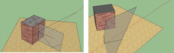

  

  Representation of mechanisms for the classical dihedral effect and the disoriented dihedral effect

5.2.2.1.5 The Use of the Generalized Interferometric Coherence

At X-band, as the traditional parameter of entropy does not seem satisfactory, we propose to use polarimetry contribution to a repeat-pass interferometric mode. Indeed, the phenomena of temporal decorrelation will be very fast in this frequency band, again sensitive to displacements of the order of a centimeter. A HIS colored representation of the interferogram obtained over the whole image of San Francisco is given in Fig. 5.14.

Fig. 5.14

Interferogram obtained over the whole image of San Francisco in HH polarization with a HSI representation. Hue: interferometric angle, Saturation: coherence level, Intensity: span

Thus, the interferometric correlation image exhibits a contrast much better than the intensity image between natural and artificial targets, as shown in Fig. 5.15 on a detail of the image. It is clear on these images that areas of parks and urban vegetation whose intensity is very high present a high decorrelation that allows distinguishing buildings.

Fig. 5.15

Image of the masks obtained from the ground truth files and applied to the performance evaluation of the different classification methods. Left: intensity on a detail of the image; right: optimum coherence on a detail of the image

The proposed solution is therefore to use optimized repeat-pass coherent polarimetry as an essential criterion for an unsupervised 2-class classification that will eventually be improved by shape criteria extracted from the span image. The optimized coherence will be obtained by one of the optimization procedures described in (Colin et al. 2006; Cloude and Papathanassiou 1998).

5.2.2.2 Experimental Results

Test sites and corresponding radar and validation data sets selected for the generation of showcases on urban classification are summarized in Table 5.3 and further described in the Appendix.

Table 5.3 Test sites and corresponding radar and validation data selected for the generation of showcases on urban classification

To use polarimetric parameters in the framework of built-up areas detection, four main features of the polarimetric analysis in the context of urban areas can be used:

• Polarimetry can distinguish between deterministic (man-made targets) and non-deterministic (natural targets).

• Built-up areas contain a lot of orientation effects that induce a non-zero polarization orientation angle (Moriyama et al. 2004). This polarization orientation angle is defined by the angle of rotation about the line of sight. It has been shown that the polarization orientation angle shifts are induced either by dihedral effects between the ground and a vertical wall that are not aligned in the along-track direction or by tilted roofs. However, the evaluation of this orientation angle is very noisy as soon as this angle becomes high.

• Double bounce effects between vertical walls and the ground give often very strong echoes in the SAR image.

• Lack of azimuthal symmetry implies that the correlation coefficient between cross-polarization and co-polarization is not equal to zero on the contrary to a flat surface or vegetated areas.

To quantify the contribution of polarimetry for building detection, we plotted ROC (Receiver Operating Characteristic) curves that are a plot of the true positive rate against the false-positive rate for the different possible cut points of a diagnostic test. These curves analyze the efficiency of using various input parameters and various distances between the two classes defined by the ground truth (built-up and natural). The closer the curve follows the left-hand border and then the top border of the ROC space, the more accurate is the test. Different distances can be calculated using different parameters: entropy, Yamaguchi, the different polarimetric correlations existing in case of non-symmetry.

The results are presented in Fig. 5.16. Then these curves clearly show that the best discriminating parameter among the tested ones is the Yamaguchi double bounce component. However, we must keep in mind that the Yamaguchi parameter does not only depend on the polarimetric content but also the powers. When we compare this parameter to the polarimetric intensity channels in Fig. 5.17, we see that it is always less efficient than the polarimetric amplitudes. That proves that polarimetric parameters that are independent of the span (entropy, correlation) give not good results here to identify alone built-up areas.

Fig. 5.16

Efficiency (ROC) of different polarimetric parameters

Fig. 5.17

ROC: Yamaguchi and intensity

Since at X-band traditional polarimetric parameter fails to identify man-made targets, we propose to use polarimetry contribution to a repeat pass interferometric mode. Indeed, the phenomena of temporal decorrelation will be very high in this frequency band, because it will be sensitive to displacements of the order of a few centimeters. Thus, the interferometric correlation image exhibits a contrast much better than the intensity image between natural and artificial targets.

The ROC curves presented in Fig. 5.18 clearly show the benefit to use interferometric coherence for discriminating buildings, at least at HH and VV polarization. Then, the benefit of polarimetry can be also considered through the use of a coherence optimization The ROC curves estimated in Fig. 5.19 also show the following points:

• It is clear that the contribution of polarimetry to optimization allows for improving the detection performance.

• Coherence optimized on a single mechanism gives similar results to the coherence optimized on two mechanisms.

• The map of HV interferometric coherence gives poor results. It is actually very noisy, maybe due to the lower signal to noise ratio that exists in this experimental polarimetric channel.

• The polarimetric coherence matrix provides also some interesting information for classification, which can outperform some pure interferometric information (e.g., in HV).

• The dual-polarimetric optimization seems to outperform slightly the full polarimetric optimization.

Fig. 5.18

ROC: comparison of intensity and interferometric coherence

Fig. 5.19

ROC: Benefit of a coherence optimization

However, the contribution of the HV should be highlighted differently. Indeed, it is clear that the contribution can be shown only in cases where the SNR is sufficient. The preliminary results of classification obtained images of San Francisco and Toulouse are given in Fig. 5.20. They will be further improved by taking into account shape criteria, for example, effective forms as the rectilinear contours of buildings.

Fig. 5.20

Results of classification of built up areas in white, over a full polarimetric image of San Francisco on the left, and over a dual-polarimetric image over Toulouse on the right

5.2.2.3 Comparison with Single-/Dual-Pol Data

The contribution of polarimetric data in comparison with single-pol data has been demonstrated in the previous section. As regards the contribution of HV versus dual-pol mode HH /VV, the situation is less clear. The ROC curves comparing the benefits of full polarimetric optimization compared to dual-pol mode presented in Fig. 5.21 show that

• For small false-positive rates (<0.5), the dual-pol optimization seems to outperform slightly the full polarimetric optimization.

• For high false-positive rates higher than 0.5, the full polarization outperforms the dual-pol mode.

Fig. 5.21

ROC curves over dual-polarimetric images of Toulouse

However, the contribution of the HV should be highlighted differently. Indeed, it is clear that the contribution can be shown only in cases where the SNR is sufficient.

The ROC curves estimated over Toulouse in dual-polarimetric mode are presented in Fig. 5.21. They also show that the second optimal coherence gives better contrast than the first one. Indeed, we should remember that Toulouse contains only bare soil and buildings, whereas San Francisco contains also vegetation and ocean. The water surface decorrelates more than soil, and then the contrast in decorrelation remains high even after optimization. Optimization can be sometimes not as efficient as expected, for example, in presence of bare soil whose optimization can improve coherence or when a polarimetric channel has an inefficient level (HV). However, averaging the optimized coherence appears to present the best performance for the detection of built-up areas. The proposed solution is therefore to use optimized repeat-pass coherent polarimetry as an essential criterion for unsupervised 2-class classification. This classification can be eventually improved by shape criteria extracted from the Span image.

5.2.2.4 Discussion on the Role of Polarimetry and on the Maturity of the Application and Conclusions

The detection of man-made targets using polarimetry has a few years now. The contribution of polarimetry to distinguish natural areas from artificial targets is well-known in classification.

This application at X-band using satellite data is far more recent with the launch of TerraSAR-X. In this context, polarimetry seems to become less effective for discriminating built-up areas. Indeed, the roughness of roofs and walls, sensitive to this scale, the different materials, and different elements that compose them, all seem to contribute to the depolarization effects or mixtures of mechanisms. In this context, it becomes difficult to predict and interpret the polarimetric answer of the urban areas.

The processing of these data at this wavelength is indeed relatively recent. There is still a lot of effort to do, especially from the point of view of modeling tools, to be able to better understand the polarimetric response at these wavelengths. In particular, there is a major effort to carry out about the influence of the wavelength related to the size of the resolution cell.

Still at X-band, it appears that the essential contribution of polarimetry is the optimization of the interferometric coherence and its use to discriminate targets based on their speed of temporal decorrelation.

5.3 3-D Rendering Over Urban Areas

5.3.1 3-D Rendering Using Coherence Optimization

5.3.1.1 Introduction, Motivation, and Literature Review

3-D rendering is a logical extension to the classification of buildings proposed in the previous section, to enrich the data necessary to monitor the growth of the urban extension. But it can also be considered as part of the diagnostic of urban areas after natural disasters such as tsunamis or earthquakes. Natural disaster monitoring and evaluation of their effects is a complex problem in urban areas because a lot of parameters can be investigated. Areas of significant changes can be detected on the basis of the exploitation of high-resolution satellite data, areas where a 3-D model can be established on a large scale by interferometry. In this context, the contribution of radar is its immediate use regardless of weather conditions or smoking out due to fires.

Polarimetry combined with interferometry can improve the product of the latter either by separation of scattering phase center, i.e., by being able to distinguish different heights in a single resolution cell or by improving the interferometric correlation map, i.e., by enhancing its value and reducing the noise level of the interferometric phase. In the latter case, to assess the benefit of polarimetry, we simply need to compare the use of the interferometric phase before and after optimization.

5.3.1.1.1 Scattering Phase Center Separation

For the separation of phase centers, the goal is to get the ground height jointly with the elevation of the roof. In this framework, the benefits of polarimetry are often compared with the benefits of pure technical image processing.

The results of techniques for phase separation will obviously depend on three factors:

• The resolution of the images. This is even the essential criterion. For instance, if the resolution is low, a vertical wall will be found synthesized in a single resolution cell. This wall will include several scattering centers, and potentially different polarimetric returns with different heights will therefore be mixed.

• The frequency. At low frequencies, the wave will not necessarily be sensitive to details. Thus, even a large resolution cell will see a limited number of mechanisms.

• The height of ambiguity for the interferometric process. The distribution of heights observed depends on this parameter: if the ambiguity height is small, then the angular diversity of the generalized coherence will be very important.

Among the techniques of phase separation, two main techniques exist:

• The ESPRIT method (Guillaso et al. 2005)

• The coherence optimization using a single mechanism that has been shown in (Colin et al. 2006) to be able to separate different phase scattering centers, under some assumptions (absence of temporal or volume decorrelation)

5.3.1.1.2 Coherence Optimization

There are different possible definitions of a generalized coherence for polarimetry and therefore other possible methods to perform an optimization. For example, we can distinguish between:

• The one mechanism optimization, proposed in (Colin et al. 2006; Qong et al. 2005).

• The initial two mechanism optimization, where the generalized coherence measures the resemblance between the response of an electromagnetic mechanism at the first antenna and another electromagnetic mechanism at the second antenna. The optimization problem has been introduced and solved to obtain the optimum scattering mechanism (Cloude and Papathanassiou 1998).

• The so-called polarization subspace method (PSM) is based on finding local maxima of the co-polar or cross-polar coherence functions. Physically, the mechanisms must be represented as an elliptic polarization transformation. The approach of the polarization state conformation (PSC) algorithm is very similar: it is based on the knowledge of the polarimetric basis transformation along with the polarization signatures of both interferometric images (Pascual et al. 2002).

All these methods can be generalized to the multibaseline case (Neumann et al. 2008).

5.3.1.1.3 Limitations

Limitations of these techniques for three-dimensional reconstruction are:

• At present, the technical phase scattering separation can distinguish up to three different heights. Practically, with current resolutions images of buildings, they are effective for a mixture of two main contributions. To be able to separate more scattering phase centers and to obtain volumetric images, it is possible to consider multibaseline approaches or tomography techniques.

• The effects of layover and interactions between buildings by the existence of urban canyons are rarely treated together on large images in a systematic way.

• The effects of statistical averaging are very influential in this type of image. A satisfactory 3-D rendering requires preliminary stages of image segmentation.

• We have seen that at X-band, the temporal decorrelation of the images is very fast.

Particularly in the resolution cells of the San Francisco images containing layover phenomenon, it is clear that the phase of the roof is mixed with the ground phase. However the ground seems to induce a high decorrelation in the mixture, and therefore its elevation cannot be estimated satisfactorily.

Thus, concerning the TerraSAR-X images of San Francisco, if the estimate of the height of the roof is possible, at present we have no satisfactory estimate of the height of the associated ground. The following image in Fig. 5.22 shows a HSI representation of the interferogram obtained over San Francisco where the interferometric phase is in hue and the optimized coherence level is in saturation. Even after an optimization, no pertinent elevation can be found on the ground. We conclude that at X-band, it is necessary to have single pass data or smaller temporal baselines to be able to provide a 3-D rendering over the whole image.

Fig. 5.22

Details of an interferogram obtained in the optimum polarization

5.3.1.2 Methodology

To perform a 3-D rendering over the entire image using a PolInSAR data set in a single pass mode, we use the following method:

• First, a prior segmentation method is proposed. It is a method of using hierarchical segmentation criteria form (essentially linear edge detection and size criteria).

• Then, an optimization method is applied to the whole image, using the calculation of coherence matrices of all pixels belonging to the same segment. We use the coherence optimization described in (Colin et al. 2006)

• Locally, for building elevation estimation, we use a scattering phase center separation method, based on the assumption that the resolution cell contains only two main scatterers at two different elevations. The algorithm is described in (Colin-Koeniguer and Trouve 2014).

Concerning this last point, we can use here the methodology that has achieved the best results. Roofs are expected to correspond either to the case of one bright point or to the case of two bright points when layover is assumed and that the resolution cell contains scatterers of the roofs mixed to scatterers from the ground. We have shown that the coherence set corresponding to the top of the roof mixed with the ground is a narrow ellipse. If polarimetric decorrelation between the two interferometric signals is very low, then the major axis of this ellipse will intersect the unitary circle into the interferometric phase of the roof and the interferometric phase of the ground. Most of the time, the ground alone is not necessarily visible. As the extension of the major axis of the ellipse is not always sufficient to ensure a robust regression, we choose to estimate separately the phase of the ground through the optimization applied to pixels belonging to the ground. This optimization enables us to find the point exp(jφ₀) where φ₀ corresponds to the interferometric phase of the ground. Then we find the intersection of the segment joining exp(jφ₀) and the optimized coherence of the roof with the unitary circle. This intersection corresponds to exp(jφ₁). The total height is deduced from φ₁ − φ₀.

5.3.1.3 Experimental Results

The 3-D rendering applications are conditioned mainly by two parameters:

• The single-pass or multipass mode of acquisitions

• The resolution

In terms of resolution, it is unlikely to achieve satisfactory results with images of resolutions higher than 3 meters. Thus we will restrict satellite data in case of the dual-pol mode of TerraSAR-X. In this context, we can evaluate the contribution of this partial polarization mode. This data will also allow us to quantify the impact of temporal decorrelation on this type of applications. We will also use data from RAMSES airborne single-pass mode and will be able to quantify the impact of multipass or single-pass mode. In both cases, we select the site of Toulouse city in south-western France. The Toulouse metropolitan area is the fifth-largest in France, one of the bases of the European aerospace industry.

Test sites and corresponding radar and validation data sets selected for the generation of showcases on 3-D urban rendering are summarized in Table 5.4 and further described in the Appendix.

Table 5.4 Test sites and corresponding radar and validation data selected for the generation of showcases on 3-D urban rendering

To validate our estimations over Toulouse with the single-pass mode, we have used a file describing building footprints and their elevation as ground truth for this application. It is a file shapefile, organized as a structure containing a list of polygonal elements. These polygons define the footprint of each building on the ground, and for each element, the minimum and maximum elevation data are given. We select the buildings of our ground truth over Toulouse that are in our PolInSAR image and that are high (> 6 m) and big (> 10 m²) enough. That gives us 140 buildings whose elevation is given with a precision of 1 m, represented in Fig. 5.23. The ambiguity height lies between 90 m for minimum ranges to 120 m for far range. In order to automatically select the pixels belonging to the building or on the ground nearby, we have registered the footprints of each building on our SAR image. An excerpt of this coregistration is given in Fig. 5.24.

Fig. 5.23

The set of buildings for elevation estimation evaluation

Fig. 5.24

Coregistration of the ground truth and the PolInSAR image

The different heights so found are evaluated in terms of the mean error in the measurement compared with heights given by ground truth, and the root mean square error. The ambiguity height on this image is about 100 meters. The three methods are also compared to the estimation computed in the single-polarimetric channels of the Pauli basis. The results are presented in Table 5.5. The best result is obtained for Method 3. Method 2 is the only one that overestimates the heights. Note that the best single-polarimetric channel for the estimation of interferometric heights is the HV. Results obtained for a 3-D rendering over the whole image are shown in Fig. 5.25.

Table 5.5 Results of building height estimation

Fig. 5.25

Three-dimensional reconstruction performed over X-band airborne data over Toulouse. The colors result from the Pauli decomposition

5.3.1.4 Comparison with Single/Dual-Polarization Data

Results indicate that estimation using a single polarization is better for HV polarization whose level is high at this frequency over a wide variety of roof surfaces. When using the partial coherence matrices obtained from HH and VV polarization only, we still can follow the same algorithm and obtain the results reported in Table 5.6. Results obtained show that the mean error is equal for dual-pol and full-pol case; however, the root mean square error is higher in the dual-pol case.

Table 5.6 Results of building height estimations: comparison full/dual/single pol

5.3.1.5 Discussion on the Role of Polarization and on the Maturity of the Application and Conclusions

Within the 3-D reconstructions field, to obtain a visually readable reconstruction thanks to SAR data, it is necessary to perform segmentation before the height reconstruction. In this context, polarimetry can be used at two levels:

• In the process of segmentation

• In the improvement of the height estimation

The application described here is still at an early stage in terms of performance evaluation. Note that unlike the applications of classification, most of the work in this area has concerned X-band. At this frequency, the cross-polarization returns seem to be particularly high. Indeed, all the polarization channels play an important role, because at this scale, numerous oriented objects will create HV returns, and depolarization effects will be high everywhere. As at X-band, the estimation of elevation requires a single-pass interferometric mode. Despite the early stage of development, this application seems to be promising as it will benefit from the improving resolutions of the new generation of satellites.

5.3.2 Building Height Estimation Using Polarimetric SAR Tomography with a Minimal Set of Images

5.3.2.1 Introduction, Motivation, and Literature Review

SAR Polarimetry (PolSAR) provides valuable information about the type of soil and urban object geometry, especially over buildings. SAR Interferometry (InSAR) may be used to determine either digital elevation models and surface deformation or the radial velocity of objects (e.g., cars). However, SAR information over dense urban environments is particularly complex due to: geometric distortions caused by the layover and shadowing phenomena, described in Fig. 5.26, complex scattering patterns within the same resolution cell (e.g., single/double-bounce scattering, volume diffusion), random aspect due to speckle effects, etc.

Fig. 5.26

Layover and shadow phenomena in urban areas

SAR tomography is the extension of conventional two-dimensional SAR imaging into three dimensions. 3-D imaging of a scene is achieved by the formation of an additional synthetic aperture in elevation and the coherent combination of images acquired from several parallel flight tracks using tomographic imaging. This technique directly retrieves the distribution of the backscattered power in the vertical direction and may be applied to estimate forest structure, building height, or layover areas induced by strong terrain slopes or discontinuities in the imaged scene.

3-D SAR focusing using tomographic processing of multibaseline interferometric data sets may be considered as a spectral estimation problem. A wide variety of spectral analysis techniques can be used to perform tomography, ranging from classical Fourier-based methods to high-resolution (HR) approaches. A recent study by (Sauer et al. 2011) proposed to apply polarimetric versions of spectral estimation methods to the airborne dual-baseline PolInSAR data sets at L-band. Results showed that using polarimetric data could improve building height estimation, both in terms of discrimination of mixed scattering responses (layover, vegetation, etc.) and determination of physical characteristics of observed media. Despite undeniable performance improvements, such an approach may have some limitations, due to the lack of statistical adaptivity of the commonly used spectral estimation methods. Firstly, as shown by (Ferro-Famil and Pottier 2007), scatterers in urban areas may have very different statistical properties that are not optimally handled by the methods proposed by (Sauer et al. 2011) and may involve estimation errors and instability. Over urban areas, backscattered signals have diverse statistical properties, e.g., coherent scatterers (e.g., point-like or double bounce scatterers) or distributed scatterers with speckle affected responses (e.g., surface or vegetation), respectively. Therefore the Conditional and Unconditional model assumptions (CM and UM) (Stoica and Nehorai 1990) may be used to estimate optimally both types of source signals.

Maximum Likelihood (ML) estimation performed under these hypotheses lead to the deterministic (Determ-ML) and stochastic (Stocha-ML) solutions, the former being statistically less efficient than the later. However, Stocha-ML achieves an optimal estimation performance at the cost of exceedingly complicated computation. Moreover, the complex scattering response from a dense urban environment leads to a mixture of various scatterers with different statistical properties that can be handled using a hybrid signal model introduced in (Sauer et al. 2011). A source signal under the hybrid assumption presents statistical properties originating partially from the UM and CM models. The performance of the MUSIC estimator degrades significantly in case of correlated signals or closely spaced signals. Moreover, processing tomographic data acquired from irregularly distributed baselines can cause ambiguous responses and sidelobe effects that may lead to erroneous interpretations and estimations.

5.3.2.2 Methodology

In order to overcome these limitations, weighted subspace techniques are of great interest, since they apply to arbitrary array structures and have a prominent performance even for highly correlated signals that are often encountered in urban areas. With an appropriate choice of weighting matrices, subspace fitting estimators possess an estimation accuracy similar to the one of conventional ML techniques (Sauer et al. 2011), at a modest computational cost. Depending on the nature of the considered subspace, different estimators may be obtained, SSF (on signal subspace) or NSF (on noise subspace), respectively, (Huang et al. 2012; Viberg and Ottersten 1991) extended the NSF estimator from the dual-polarization case (Swindlehurst and Viberg 1993) to the Fully Polarimetric (FP) case and also provided an analytic solution that maintains its optimization complexity to the one of the single-polarization (SP) case (Huang et al. 2012). Using a critical and minimal tomographic configuration consisting of only 3 PolSAR data sets, this FP-NSF estimator is applied to estimate building heights and scattering mechanisms over dense urban areas.

5.3.2.3 Experimental Results

The application data set was acquired by the DLR’s experimental SAR (E-SAR) system over the city of Dresden (see Table 5.7) in a dual-baseline fully polarimetric interferometric configuration with a small baseline equal to 10 m and a large one of 40 m, which form a small-size irregular array. The acquired SAR images are of intermediate resolution (3 m in azimuth and 2.2 m in range), leading to a sum of diverse polarimetric and statistical contributions within each resolution cell. The scene consists of buildings, trees, parks, grassland, and some bare surfaces like sports fields, as depicted in Fig. 5.27.

Table 5.7 Test sites and corresponding radar and validation data selected for the generation of showcases on building height estimation with PolTomoSAR

Fig. 5.27

Optical and SAR images of the city of Dresden. Optical images: Copyright Bing Maps

Two buildings facing the radar flight track are studied over a set of range bins corresponding to the yellow bar in Fig. 5.28. Tomograms over this test line are computed by using the dual-baseline Fully Polarimetric (FP) data sets and the FP NSF method and then projected in ground range in Fig. 5.29. Due to the very low dimension of the observation space, conventional model order selection techniques may fail to accurately determine the number of scatterers within one resolution cell. For this reason, the number of scatterers is fixed to 2 over the selected range bins. The resulting tomograms depict the building shape and scattering patterns using the reflectivity in Fig. 5.29 (left) and α values in Fig. 5.29 (right). Compared with the lidar profile (black line), the building height and its shape are quite well estimated based on this dual-baseline intermediate-resolution data set. At the wall-ground interaction, strong reflectivities and high α values are due to the powerful double-bounce reflection. Over the roofs and surfaces, the α value decreases indicating surface scattering.

Fig. 5.28

Test area containing buildings facing the acquisition flight path: optical image (left) and Pauli-coded SAR image (right)

Fig. 5.29

Tomograms estimated by FP-NSF method: reflectivity tomogram (left) with scale: 25–110 dB and α tomogram with scale: 0–90° (right)

The 3-D reconstruction over an urban zone shown in Fig. 5.30 has been run using the FP-NSF tomographic estimator with model order equal to 2, and the corresponding results are depicted in Fig. 5.31. From the α values in Fig. 5.31 (right), scattering mechanisms can be distinguished in the vertical direction (unlike conventional 2-D polarimetric analysis) that allows to discriminate for instance double bounce scattering at the wall-ground interaction as well as over some of roofs with complex structures. Over the whole test zone, the surface elevation is estimated by the FP-NSF estimator considering two sources, which matches very well with lidar elevation data, as can be observed in Fig. 5.32. A 3-D reconstruction of a group of buildings is validated against lidar in Fig. 5.33.

Fig. 5.30

Another urban area under study. Optical image (left) and Pauli-coded SAR image (right)

Fig. 5.31

3-D tomographic reconstruction using dual-baseline PolInSAR data sets, shaded by surface elevation (left) and α value (right)

Fig. 5.32

Lidar surface elevation (right) and estimated surface elevation by FP-NSF estimator (left)

Fig. 5.33

3-D reconstruction: lidar (left) and FP-NSF estimator (right)

5.3.2.4 Comparison with Single/Dual-Polarization Data

The VV reflectivity tomogram in Fig. 5.34 (left) shows an incomplete building shape especially on the top of the buildings, leading to an inaccurate estimation of the building height due to missed patterns. The HH tomogram is affected by spurious sidelobes which degrade building height estimation too. However, the tomographic profile obtained from fully polarimetric data set permits to guess correctly building shapes with a consistent height estimation compared to the lidar profile. This fact reveals that fully polarimetric dual-baseline configuration improves significantly the tomographic accuracy, compared with single-polarization ones, and provides additional information, related to scattering mechanisms, which helps to better characterize building features, like geometrical shapes as well as dielectrical properties, etc.

Fig. 5.34

Single-polarization HH (left), VV (middle) and fully polarimetric (right) reflectivity tomograms with scale: 25–110 dB

5.3.2.5 Discussion on the Role of Polarization and on Maturity of the Application and Conclusions

Polarimetric SAR tomography (PolTomoSAR) is a very interesting approach to analyze complex 3-D environments, like urban environments, forested areas, etc. As it is demonstrated in this section, powerful spectral analysis techniques can be used to efficiently separate responses from scatterers located at different elevations in very severe scenarios, i.e., with only three images. Combining tomographic processing with polarimetric diversity provides a significant gain in performance as the 3-D imaging process adapts to the polarimetric properties of the scatterers to be imaged, i.e., adaptively maximizes SNR and estimation accuracy. Fully polarimetric tomography permits to further discriminates closely spaced scatterers having diverse polarimetric responses and is less sensitive to artifacts and spurious sidelobes, compared to single-polarization approaches. Moreover, PolTomoSAR results can be processed through usual polarimetric approaches, like polarimetric decompositions and others, in order to characterize, identify scatterers, and provide interpretation of scattering mechanisms.

PolTomoSAR analysis of urban environments has been conducted over nearly a decade, with very different spectral estimation approaches and acquisition configurations, and may be considered as mature. The approach used here provides very high vertical resolution and a robust estimation of different parameters of urban environments, like building heights and scattering mechanisms. PolTomoSAR techniques can be extended to different applications such as subsurface observation and forestry remote sensing, under foliage imaging and object detection (Huang et al. 2012).

5.4 Subsidence Monitoring

Since its conception in the late 1990s, differential SAR Interferometry (DInSAR) is an established technique useful for the monitoring of deformation episodes over wide areas (Ferretti et al. 1999, 2001). PSI techniques exploit the phase information of a stack of interferograms, obtained from a set of SAR images acquired at different dates, to retrieve accurate information of the ground deformation evolution along time. In this framework and mainly due to decorrelation phenomena, any advanced DInSAR technique is constrained by the number and the quality of trustful points from where reliable information of deformation can be retrieved. Two main criteria are available in the literature to perform adequate pixel quality estimation. In the first approach, the phase quality is assessed through the coherence estimator applied to each interferometric pair (Mora et al. 2003; Berardino et al. 2002). In the second approach, the phase quality is associated with the amplitude dispersion index DA of the images (Ferretti et al. 1999), often used in urban environments, where it is common to find point-like, deterministic scatterers (called Persistent Scatterers, PS) associated with strong and stable backscattering from man-made structures. The higher the interferometric coherence or, accordingly, the lower the DA, the better the phase quality and, thus, the most reliable the deformation process estimation.

Due to the lack of polarimetric SAR (PolSAR) data sets, the use of DInSAR techniques has been traditionally limited to the single-polarization approach.

However, the scenario has changed with the launch of new satellites with polarimetric capabilities, such as TerraSAR-X, RADARSAT-2, ALOS-PALSAR, and the upcoming launch of Sentinel-1, ALOS-2, and RADARSAT Constellation Mission. The new polarimetric diversity can be exploited in order to enhance the performance of conventional PSI approaches.

5.4.1 Improvement of Differential SAR Interferometry for Subsidence Monitoring with Polarimetric Optimization Techniques

5.4.1.1 Introduction, Motivation, and Literature Review

The application of polarimetric optimization methods has led to an improvement in the density but also in the quality of the deformation process retrieval (Pipia et al. 2009; Navarro-Sanchez et al. 2010; Navarro-Sanchez and Lopez-Sanchez 2011a, b, 2012; Iglesias et al. 2012; Monells et al. 2012) .

This section describes the three polarimetric optimization methods available in the literature when PolSAR data sets are available. The methods are referred as Best (Pipia et al. 2009), Equal Scattering Mechanism (ESM) (Colin et al. 2006) and Sub-Optimum Scattering Mechanism (SOM) (Sagues et al. 2000). Their exploitation for DInSAR applications is addressed with both the coherence stability and DA pixel selection criteria. The objective is to improve the quality of the interferograms through the proper combination of the available polarimetric channels. The optimization techniques will use the phase quality estimators as figures of merit. Deformation maps obtained from fully polarimetric data sets will be compared with those obtained with the traditional single-polarimetric approaches in order to show the benefits of the former. In addition, the performances of dual-polarimetric data are also evaluated.

5.4.1.1.1 Classical Differential SAR Interferometry

DInSAR processing aims at obtaining the temporal evolution of deformation episodes, together with the topographic error and atmospheric artifacts, from a stack of multi-temporal differential interferograms. In this framework, a usual approach, among others, is the Coherent Pixels Technique (CPT) (Mora et al. 2003; Blanco et al. 2008). CPT can work with either the coherence or the amplitude-based pixel selection criteria. Similarly to other DInSAR algorithms, a linear model, which includes the linear deformation term and the topographic error of the DEM used to generate the differential interferograms, is adjusted to the interferometric data through a minimization process (Blanco et al. 2008). Once the linear deformation term and the topographic error have been determined for the selected pixels, in a second step the deformation time series and the atmospheric phase screen are derived for all selected pixels leading to a complete characterization of the deformation process.

5.4.1.1.2 Polarimetric Differential SAR Interferometry

Working at the PolSAR acquisition level, the scattering matrix S, which indicates the polarimetric information associated to each pixel of the scene, can be defined, in the orthogonal horizontal and vertical polarization basis {H,V}, as (Lee and Pottier 2009).

$$ {\mathbf{S}}_{\left({\hat{\mathbf{u}}}_{\mathrm{H}},{\hat{\mathbf{u}}}_{\mathrm{V}}\right)}=\left[\begin{array}{cc}{S}_{\mathrm{H}\mathrm{H}}& {S}_{\mathrm{H}\mathrm{V}}\\ {}{S}_{\mathrm{H}\mathrm{V}}& {S}_{\mathrm{V}\mathrm{V}}\end{array}\right] $$

(5.5)

In this context, it is possible to indicate the scattering matrix S in another generic orthogonal basis {X,Y} through a unitary transformation (Lee and Pottier 2009; Kostinski and Boerner 2009).

$$ {\mathbf{S}}_{\left(\hat{\mathbf{x}},\hat{\mathbf{y}}\right)}=\left[\begin{array}{cc}{S}_{\mathrm{XX}}& {S}_{\mathrm{XY}}\\ {}{S}_{\mathrm{XY}}& {S}_{\mathrm{YY}}\end{array}\right]={{\mathbf{U}}_2}^T{\mathbf{S}}_{\left({\hat{\mathbf{u}}}_{\mathrm{H}},{\hat{\mathbf{u}}}_{\mathrm{V}}\right)}{\mathbf{U}}_2 $$

(5.6)

where (⋅)^T refers to the vector transposition and the matrix transformation U₂ can be expressed in terms of the orientation and ellipticity angles (ψ, χ) of the polarization ellipse by

$$ {\mathbf{U}}_2=\left[\begin{array}{cc}\cos \psi & -\sin \psi \\ {}\sin \psi & \cos \psi \end{array}\right]\left[\begin{array}{cc}\cos \chi & j\sin \chi \\ {}j\sin \chi & \cos \chi \end{array}\right]\left[\begin{array}{cc}{e}^{+j{\phi}_0}& 0\\ {}0& {e}^{-j{\phi}_0}\end{array}\right]. $$

(5.7)

From an interferometric point of view, if two PolSAR acquisitions obtained at different times i = 1, 2 are available, the so-called scattering vector k_i can be defined as a vectorization of the scattering matrix S as

$$ {\mathbf{k}}_i=\frac{1}{\sqrt{2}}{\left[{S}_{\mathrm{HH},i}+{S}_{\mathrm{VV},i},{S}_{\mathrm{HH},i}-{S}_{\mathrm{VV},i},2{S}_{\mathrm{HV},i}\right]}^T. $$

(5.8)

The scattering vector k_i can be projected onto an unitary projection vector w obtaining a generic scattering coefficient ${S}_i={\mathbf{w}}_i^{\ast T}{\mathbf{k}}_i$ for each pair of images i = 1, 2, where ^∗T is the conjugate transpose operator. At this stage, the PolInSAR vector between two PolSAR acquisitions is defined by (Cloude 2009; Qong et al. 2005)

$$ {\mathbf{k}}_6={\left[{\mathbf{k}}_1^T,{\mathbf{k}}_2^T\right]}^T. $$

(5.9)

Once the PolInSAR vector k₆ is defined, under the assumption of spatial homogeneity and ergodicity, the 6 × 6 PolInSAR coherency complex matrix T₆ is defined as

$$ {\mathbf{T}}_6=E\left\{{\mathbf{k}}_6{\mathbf{k}}_6^{\ast T}\right\}=\left[\begin{array}{cc}{\mathbf{T}}_{11}& {\boldsymbol{\Omega}}_{12}\\ {}{\boldsymbol{\Omega}}_{12}^{\ast T}& {\mathbf{T}}_{22}\end{array}\right] $$

(5.10)

T ₁₁ and T₂₂ refer to the coherency matrices of each PolSAR data set and Ω₁₂ indicate the polarimetric interferometric coherency matrix. In this context, the expression of the classical interferometric coherence can be generalized taking into account its polarimetric dependence

$$ \gamma \left({\mathbf{w}}_1,{\mathbf{w}}_2\right)=\frac{{\mathbf{w}}_1^{\ast T}{\boldsymbol{\Omega}}_{12}{\mathbf{w}}_2}{\sqrt{\left({\mathbf{w}}_1^{\ast T}{\mathbf{T}}_{11}{\mathbf{w}}_1\right)\left({\mathbf{w}}_2^{\ast T}{\mathbf{T}}_{22}{\mathbf{w}}_2\right)}} $$

(5.11)

Notice that different projection vectors between the different acquisitions of the interferogram, w₁ ≠ w₂, may lead to the introduction of a polarimetric contribution in the interferometric phase, due to a phase center change within the same resolution cell. Thus, ensuring the same projection vector along the whole stack of interferograms, w = w₁ ≠ w₂, is mandatory for Polarimetric Differential SAR Interferometry (PolDInSAR) applications. Under this restriction, (5.11) can be rewritten as

$$ \gamma \left(\mathbf{w}\right)=\frac{{\mathbf{w}}^{\ast T}{\boldsymbol{\Omega}}_{12}\mathbf{w}}{\sqrt{\left({\mathbf{w}}^{\ast T}{\mathbf{T}}_{11}\mathbf{w}\right)\left({\mathbf{w}}^{\ast T}{\mathbf{T}}_{22}\mathbf{w}\right)}}. $$

(5.12)

In the framework of PolDInSAR, polarimetric optimization methods seek to optimize the generalized expression of the coherence (5.12). The first approach explores the whole space of projection vectors w looking for the one providing the highest value of coherence. The second one explores all the polarimetric transformations given by (5.6) and again looks for the one providing the maximum value of coherence. Meanwhile, when working with point-like scatterers, the expression of the D_A can be also generalized (Navarro-Sanchez et al. 2010; Navarro-Sanchez and Lopez-Sanchez 2011a, b, 2012, 2013; Navarro-Sanchez et al. 2014) as

$$ {\displaystyle \begin{array}{l}{D}_A\left(\mathbf{w}\right)=\frac{\sigma_A}{m_A}=\frac{1}{\left\langle \left|{\mathbf{w}}^{\ast T}\mathbf{k}\right|\right\rangle}\sqrt{\frac{1}{N}\sum \limits_{i=1}^N{\left(\left|{\mathbf{w}}^{\ast T}{\mathbf{k}}_i\right|-\left\langle \left|{\mathbf{w}}^{\ast T}\mathbf{k}\right|\right\rangle \right)}^2}\\ {}\kern2.75em \mathrm{where}\kern0.75em \left\langle \left|{\mathbf{w}}^{\ast T}\mathbf{k}\right|\right\rangle =\frac{1}{N}\sum \limits_{i=1}^N\left|{\mathbf{w}}^{\ast T}{\mathbf{k}}_i\right|\end{array}} $$

(5.13)

where σ_A is the standard deviation and m_A is the mean of the amplitude time series. In this case the objective is, as stated in the coherence case, to find the projection vector or the polarimetric transformation that minimizes the generalized expression of D_A.

5.4.1.2 Methodology

5.4.1.2.1 Stability Optimization Methods

In this section, the basis of the different polarimetric optimization methods for PolDInSAR applications with the coherence stability pixel selection approach is addressed.

The first approach, referred as Best, is based on selecting the polarimetric channel providing the highest temporally averaged coherence value for each pixel along the whole stack of interferograms. Consequently, the original three interferograms (one per polarimetric channel) are mixed in a new interferogram where the phase of each pixel corresponds to the channel providing the highest temporally averaged coherence. In order to avoid changes in the phase centers, the polarization mechanism for each pixel has to be equal in all the interferograms of the data set.

The second approach, which is referred as Equal Scattering Mechanism (ESM), consists on finding the projection vector w that maximizes the generalized expression of the coherence (5.12). The solution must be obtained using numerical methods since the maximization problem has no analytical solution. The simplest approach consists on parameterizing the projection vector w to obtain all the possible values of the generalized coherence. The parameterization presented in (Cloude and Papathanassiou 1998) can be used to ensure the unitarity of the projection vector

$$ \mathbf{w}=\left[\begin{array}{c}\cos \alpha \\ {}\sin \alpha \cos \beta {e}^{j\delta}\\ {}\sin \alpha \sin \beta {e}^{j\gamma}\end{array}\right]\kern1.25em \left\{\begin{array}{c}0\le \delta \le \pi, -\pi \le \gamma <\pi, \\ {}0\le \alpha \le \frac{\pi }{2},0\le \beta \le \pi \end{array}\right. $$

(5.14)

The optimum projection vector will be the one providing the maximum coherence. The main drawback of this approach is its high computational cost. To face this problem, the solution presented in (Colin et al. 2006) which makes use of an iterative process to find the optimum projection vector w is proposed. This approach assumes that the two coherency matrices T₁₁ and T₂₂ are similar, which is accomplished when polarimetric stability applies. Under this hypothesis, the estimated complex differential coherence is approximated by

$$ \hat{\gamma}\left(\mathbf{w}\right)=\frac{{\underline {\mathbf{w}}}^{\ast T}{\boldsymbol{\Omega}}_{12}\underline {\mathbf{w}}}{{\underline {\mathbf{w}}}^{\ast T}\mathbf{T}\underline {\mathbf{w}}}\kern0.75em \mathrm{where}\kern0.75em \mathbf{T}=\frac{{\mathbf{T}}_{11}+{\mathbf{T}}_{22}}{2}, $$

(5.15)

where $\left|\hat{\gamma}\right|<\left|\gamma \right|$ and the interferometric phase provided by both estimators is preserved. In the framework of PolDInSAR applications, an extension of the method introduced by Colin et al. in (Colin et al. 2006) to the multi-temporal case may be considered. The extension presented by Neumann et al. in (Neumann et al. 2008) aims to optimize the temporally averaged coherence instead of the coherence of each interferogram separately. Once the optimum projection vector w_{opt, ESM} is found, the coherence is obtained through (5.12), and the interferometric phase is given by

$$ {\phi}_{ESM}=\arg \left({\mathbf{w}}_{opt, ESM}^{\ast T}{\boldsymbol{\Omega}}_{12}{\mathbf{w}}_{opt, ESM}\right). $$

(5.16)

On the other hand, when polarimetric stability does not apply the optimized differential phase may be affected by the difference of polarimetric behavior, leading to an erroneous phase value. An alternative method referred as Sub-Optimum Scattering Mechanism (SOM) (Sagues et al. 2000) is proposed in order to overcome these restrictions. The algorithm is based on exploring the entire possible polarimetric basis, departing from S_hv and sweeping all the values of ellipticity and orientation angles. This will consider all the possible polarization states of the propagating wave. The key step resides in looking for the polarization basis transform providing the highest temporally averaged coherence value among all the co-polar and cross-polar realizations

$$ \left|{\overline{\gamma}}_{SOM}\right|=\underset{\left(\psi, \chi \right)}{\max}\left\{\left|{\overline{\gamma}}_{\mathrm{XX}}\left(\psi, \chi \right)\right|,\left|{\overline{\gamma}}_{\mathrm{XY}}\left(\psi, \chi \right)\right|\right\} $$

(5.17)

The subscripts XX and XY refer to the co-polar and cross-polar channels in the new (ψ, χ) polarization basis, respectively. This method could be seen as a subspace of the ESM approach.

5.4.1.2.2 Amplitude Dispersion Optimization Methods

In this section, the basis for the adaptation of the three optimization methods presented before will be particularized for the D_A pixel selection criterion approach.

As in the coherence case, the Best approach is the simplest way to face the polarimetric optimization problem. It is based on selecting the interferometric phases of the polarimetric channel providing the minimum D_A.

The second approach, ESM, explores the whole polarimetric space looking for the projection vector w that minimizes the generalized D_A expression (5.13). To solve this problem, there is no analytical solution. Hence, the optimization problem must be solved by brute force, parameterizing the projection vector as seen in (5.12). As in the coherence case, the main drawback of this approach is the computational cost since a 4-D space needs to be explored. For this reason, the adaptation of the SOM approach is an appropriate alternative. As seen in the coherence stability case, the method consists in sweeping all the possible orientation and ellipticity angles in order to reach a scattering matrix in a new polarization basis, which provides a minimum D_A value among all the co-polar D_{A, aa} and cross-polar D_{A, ab} indices. With this approach, the computational load is highly reduced since the solution now consists in exploring a 2-D space corresponding to all possible orientation and ellipticity angles.

5.4.1.3 Experimental Results

The PolSAR data set used in this work consists of 34 fully polarimetric RADARSAT-2 images, from January 2010 to May 2012, that correspond to the metropolitan area of Barcelona, Northeastern Spain. RADARSAT-2 works at C-Band, with a resolution of 5 meters in both range and azimuth directions and a revisiting time of 24 days. Selected test sites and data sets are summarized in Table 5.8 and further described in the Appendix.

Table 5.8 Test sites and corresponding radar and validation data selected for the generation of showcases on urban subsidence monitoring

This section shows the PolDInSAR results obtained using the different polarization optimization techniques described previously with both the coherence and amplitude approaches. Once the phase optimization is performed in the pixel selection step, the classical DInSAR processing can be applied to the new stack of optimized interferograms, since there are no differences from the single-polarimetric case.

The pixel selection with the coherence approach has been performed establishing a threshold of 0.75, which corresponds to a phase standard deviation of 5° with the 9 × 5 multi-look window used (Hanssen 2001). To highlight the performances of the different optimization methods, a quite restrictive threshold has been established. Table 5.9 shows the pixel density obtained for each method. Notice how with polarimetric optimization techniques, it is possible to reach an increase in the number of selected pixels of a 2.7 factor compared with the single-polarization case.

Table 5.9 Coherence stability pixel selection statistics for each method. (%) refers to the total number of pixels

Figure 5.35 shows a comparison of final DInSAR deformation maps obtained using the S_hh single-polarimetric channel and the three different optimization methods. The deformation pattern is almost identical in all cases, and the main differences lay in the pixel densities shown in Table 5.9. Different deformation bowls can be observed in the figure; the most severe is in the airport and in the harbor area. Some weaker deformations are observed in the city. In the North-East part of the image, interesting subsidence that follows the track of a metro line under construction is identified. Since the affected area is narrow, it is difficult to detect when the density of pixels is low, such as in the single-polarimetric case. The optimization methods largely increase the number of selected pixels leading thus to a better determination of the deformation bowl extension and its characterization.

Fig. 5.35

Linear velocity retrieved over Barcelona, from January 2010 to May 2011. Using the hh polarimetric channel (a) or the Best (b), SOM (c) and ESM (d) mean coherence stability optimization methods

Regarding the amplitude-based approach, a D_A threshold of 0.25, which corresponds to a phase standard deviation of 15° (Hanssen 2001), has been used. Notice how the differences among the different methods are more substantial for this case; see Table 5.10. The ESM approach increases in a factor of seven the number of pixels from the single-polarimetric case. As in the coherence stability case, this pixels’ density increase justifies the use of PolSAR data in the DInSAR framework.

Table 5.10 D_A pixel selection statistics for each method. (%) refers to the total number of pixels

Finally, Fig. 5.36 shows the linear deformation maps using each optimization approach in the area within the city of Barcelona commented before. All approaches are able to determine the deformation bowls with similar values of terrain deformation. The main differences come from the larger pixels’ densities obtained when using the advanced polarimetric optimization methods. ESM provides the larger improvement in number of pixels, and consequently the deformation map allows precisely determining the extension of the deformation bowl along the new underground line. The different deformation bowls observed in the figure match the path followed by the tunnel, and the widest bowl, also with the highest subsidence, is located over a new underground station.

Fig. 5.36

Linear velocity retrieved from the RADARSAT-2 PolSAR data set. Using the hh polarimetric channel (a) and the Best (b), SOM (c) or ESM (d) DA-based optimization methods for the DInSAR processing. The orange line shows the path of the new underground line

5.4.1.4 Comparison with Single/Dual-Polarization Data

The usage of fully polarimetric data imposes some limitations in the sensors regarding the swath extension, basically reduced by a factor of two if compared with the single or dual-pol cases. This section presents a comparison between the performances of full and dual-pol data in terms of pixels’ density. Fully polarimetric data entails covering the entire polarimetric space; hence the optimum value in terms of the phase quality can be reached. If only dual-pol data are available, the result is obviously suboptimum, but the complexity of the optimization process is significantly reduced. Moreover, dual-pol configurations are in general more efficient in terms of coverage.

To simulate the performance of dual-polarimetric products, the fully polarimetric data set available has been narrowed down selecting either the two direct channels (HH/VV) or a direct channel and a cross-polar channel (HH/HV or VV/VH). The first option presents the same swath restrictions than the full-pol case. The comparison is based on the optimization process performance, so swath differences are omitted. The ESM approach, under the DA pixel selection criterion, is selected for the comparison since it provides the best performance. Table 5.11 shows the results after the pixel selection step. Results reveal that both fully polarimetric and dual-polarimetric data are suitable for phase quality optimization techniques since they clearly outperform the single-polarimetric case. As expected, the dual-pol optimization does not produce the same improvement in pixels density than the full-pol case. For this particular data set, there is roughly a factor of two between the dual-pol and the full-pol densities. On the other hand, the performance among the dual-polarimetric configurations is rather similar, being the HH-VV combination slightly better than the ones involving the cross-polar channel. For this reason, despite the major computational load and the higher complexity in the algorithms, the use of fully polarimetric data is strongly recommended.

Table 5.11 Amplitude dispersion pixel selection for dual VS fully polarimetric configurations. The % of pixels is over the total pixels considered

5.4.1.5 Discussion on the Role of Polarization and on the Maturity of the Application and Conclusions

General polarimetric optimization methods for its application in DInSAR processing have been evaluated. The three different optimization techniques have been put forward using RADARSAT-2 fully polarimetric data and working with both the coherence stability and the amplitude-based pixel selection criteria.

With the proper combination of the available polarimetric channels, the proposed polarimetric optimization methods demonstrate their capability to enhance the quality of DInSAR results. First, it is possible to obtain a higher density of pixels compared with the single-polarization case. Moreover, the quality of the interferometric phase is also improved, leading to more precise deformation maps. This fact provides major robustness in DInSAR algorithms and is a key factor to better determine and characterize deformation bowl extensions.

Concerning the comparison of fully polarimetric and dual-polarimetric data, the use of fully polarimetric data is strongly recommended since it clearly improves the DInSAR results.

5.4.1.6 Acknowledgment

This research work received partial support from the SafeLand project funded by the Commission of the European Communities, grant agreement 226479, from the Big Risk project, contract number BIA2008-06614, the project TEC2011-28201-C02-01 and the grant BES-2009-015990 associated with the project TEC2008-06764-C02-01, both funded by the Spanish MICINN and FEDER funds. The RADARSAT-2 images were provided by MDA in the framework of the scientific project SOAR-EU 6779.

5.4.2 Ground Deformation Estimation Using Polarimetric Persistent Scatterers Interferometry

5.4.2.1 Introduction, Motivation, and Literature Review

In this section, we present a general framework for improving PSI through polarimetry. The proposed approach seeks the optimization of the parameters used as quality criteria for the initial pixel selection, with the consequent improvement in terms of density of points with valid deformation results. Moreover, disposing of denser distributions of PS or CP constitutes an advantage for the data processing itself, since many stages (e.g., phase unwrapping, atmospheric phase screen removal, interpolations, etc.) are carried out more robustly and accurately than with sparse distributions of pixels. Consequently, final deformation values are also more accurate in such conditions.

First works on single-pol PSI can be found in (Ferretti et al. 1999, 2001) which make use of an amplitude dispersion criterion (D_A) for persistent scatterers selection. D_A criterion may not be suitable for non-urban areas, where strong point-like scatterers are less common, or when only a small set of SAR images of the area under study is available; hence D_A estimates may be biased. To overcome these drawbacks, many techniques based on average interferometric coherence ($\left|\overline{\gamma}\right|$) were proposed (Mora et al. 2003; Berardino et al. 2002). Points selected using this method are usually referred as coherent pixels (CP) and correspond to stable distributed scatterers, rather than point-like ones. Notice that maximum likelihood estimation of interferometric coherences generally requires averaging of neighboring samples, consequently spatial resolution is degraded. Alternative PSI approaches can also be found in (Hooper et al. 2004, 2007), where a phase coherence analysis is used in order to refine the initial PS selection, and (Ferretti et al. 2011) where joint analysis of PS and CP is addressed. A reference book in this area is (Kampes 2006).

The first application of polarimetry to urban PSI was proposed in (Perissin and Ferretti 2007) which made use of ENVISAT incoherent dual-pol data to recognize target physical features and to classify PS. Another PS classification strategy supported by polarimetry was also presented in (Dheenathayalan and Hansen 2011) in the context of building-versus-ground relative movement estimation, using TerraSAR-X coherent dual-pol data.

To further exploit polarimetric diversity at initial PSI processing stages, an algorithm aiming to increase the quality and number of pixels pre-selected for PSI processing was introduced in (Pipia et al. 2009). The proposed algorithm consisted in selecting, from the set of polarimetric channels provided by the sensor, the one that optimizes the average interferometric coherence for each pixel. The algorithm was tested using dual-pol (HH, VV) ground-based SAR data, achieving a significant improvement in the density of selected CP and demonstrating for the first time the potentials of polarimetry for PSI. Extending that idea, in (Navarro-Sanchez and Lopez-Sanchez 2012; Navarro-Sanchez et al. 2014), a generic method for polarimetric PSI optimization was proposed and tested using a set of TerraSAR-X dual-pol images. For each pixel, the algorithm finds the optimum channel as a linear combination of the set of channels measured by the sensor. That algorithm, which is employed in this work, can be adapted to optimize any parameter used as quality criterion and can be used as a pre-processing step to any known PSI technique. Following this line, an efficient search of the optimum channel was also addressed, and results using fully polarimetric data were presented in (Navarro-Sanchez et al. 2014; Monells and Mallorqui 2013), showing a remarkable improvement compared to dual-pol data in terms of density of PS and CP.

Concerning other pixel selection criteria, the normalized average Polarization Phase Difference (PPD) was proposed in (Samsonov and Tiampo 2011) for selecting only those pixels clearly dominated by odd and even bounce scattering mechanisms. In (Navarro-Sanchez and Lopez-Sanchez 2011b), a polarimetric stationarity test was proposed as a means to refine PS and CP selection. Similarly, a complete study of the temporal evolution of the polarimetric behavior of an urban area was carried out in (Pipia et al. 2012) using ground-based SAR data, and a filtering strategy was proposed to minimize the presence of non-stationary backscattering processes. Finally, in (Navarro-Sanchez and Lopez-Sanchez 2013), an adaptive spatial speckle filtering approach driven by polarimetric temporal statistics is exploited as a pre-processing stage before polarimetric optimization, which allows to process simultaneously both optimized PS (point-like targets) and CP (homogeneous, distributed scatterers), obtaining a significant increase in the final density of points and spatial coverage of deformation maps.

5.4.2.2 Methodology

The main objective of the polarimetric approach used here for PSI is to maximize the quality and number of PS or CP selected as reliable a priori, by optimizing the parameters used as a selection criterion. In (46), (48) we proposed a general framework for PSI polarimetric optimization, starting from the concept of polarimetric (or vector) interferometry introduced in (Cloude and Papathanassiou 1998). Let k be a pixel’s target vector obtained by projecting its scattering matrix S onto the Pauli basis. For fully polarimetric data, it is given by:

$$ \mathbf{k}=\frac{1}{\sqrt{2}}\left[\begin{array}{c} HH+ VV\\ {} HH- VV\\ {}2 HV\end{array}\right] $$

(5.18)

where HH and VV stand for the horizontal and vertical co-polar channels, respectively, and HV is the cross-polar channel. Notice that we assume HV = VH due to reciprocity. In order to generate an interferogram, k can be projected onto a unitary complex column vector ω, resulting in:

$$ \mu ={\boldsymbol{\upomega}}^{T\ast}\mathbf{k} $$

(5.19)

where and μ is a scalar complex scattering coefficient. As a scalar complex, μ is analogous to single-pol data, so we can make use of any known PSI technique by applying it to μ. Therefore, the proposed PSI optimization approach consists in finding, for each pixel, the projection vector ω that optimizes the parameter considered as the quality criterion when computed for μ.

To facilitate the search of the optimum projection vector, we can parameterize ω in a way we ensure it is unitary, and we take into account all possible unambiguous combinations:

$$ \boldsymbol{\upomega} =\left[\begin{array}{c}\cos \left(\alpha \right)\\ {}\sin \left(\alpha \right)\cos \left(\beta \right){e}^{i\delta}\\ {}\sin \left(\alpha \right)\sin \left(\beta \right){e}^{i\psi}\end{array}\right],\kern1em \left\{\begin{array}{c}0\le \alpha \le \frac{\pi }{2}\\ {}0\le \beta \le \frac{\pi }{2}\\ {}-\pi \le \delta <\pi \\ {}-\pi \le \psi <\pi \end{array}\right. $$

(5.20)

Therefore, the problem is reduced to find four real parameters, α, β, δ, and ψ whose range is finite and known and which value is related to the geometric and electromagnetic properties of the target (Cloude 2009). We have adapted this formulation to the dual-pol case, as the TerraSAR-X data at our disposal. For dual-pol data, the target vector is given by:

$$ \mathbf{k}=\frac{1}{\sqrt{2}}\left[\begin{array}{c} HH+ VV\\ {} HH- VV\end{array}\right] $$

(5.21)

and the projection vector can be parameterized as:

$$ \boldsymbol{\upomega} =\left[\begin{array}{c}\cos \left(\alpha \right)\\ {}\sin \left(\alpha \right){e}^{i\psi}\end{array}\right],\kern1em \left\{\begin{array}{c}0\le \alpha \le \frac{\pi }{2}\\ {}-\pi \le \psi <\pi \end{array}\right. $$

(5.22)

so in this case the search is reduced to just two real parameters, α and ψ.

The optimization approach is tested here for the two most commonly used criteria of selection: the average interferometric coherence and the amplitude dispersion index. In the context of polarimetric interferometry, the average coherence $\overline{\left|\gamma \right|}$ can be expressed as:

$$ \overline{\left|\gamma \right|}=\frac{1}{K}\sum \limits_{k=1}^K\left|{\gamma}_k\right|,\kern1em \mathrm{with}\kern0.5em {\gamma}_k\left(\boldsymbol{\upomega} \right)=\frac{{\boldsymbol{\upomega}}^{\dagger }{\boldsymbol{\Omega}}_{ij}\boldsymbol{\upomega}}{\sqrt{{\boldsymbol{\upomega}}^{\dagger }{\mathbf{T}}_{ii}\boldsymbol{\upomega}}\sqrt{{\boldsymbol{\upomega}}^{\dagger }{\mathbf{T}}_{jj}\boldsymbol{\upomega}}} $$

(5.23)

where subscript k denotes the k-th interferogram obtained by combining images i and j. Polarimetric coherency matrices T_ii, T_jj and polarimetric interferometric cross-correlation matrix Ω_ij are defined as in (7):

$$ {\mathbf{T}}_{ii}=E\left\{{\mathbf{k}}_i{\mathbf{k}}_i^{T\ast}\right\},\kern1em {\mathbf{T}}_{jj}=E\left\{{\mathbf{k}}_j{\mathbf{k}}_j^{T\ast}\right\},\kern1em {\boldsymbol{\Omega}}_{ij}=E\left\{{\mathbf{k}}_i{\mathbf{k}}_j^{T\ast}\right\} $$

(5.24)

where E{⋅} is the expectation operator. As these expectations cannot be computed in practice, they are usually replaced by their maximum-likelihood estimates, given by the empirical mean evaluated using L samples of the target vectors (multi-look). Despite a larger number of looks generally implies better estimates (if the averaged area is sufficiently homogeneous), averaging also degrades spatial resolution, so a trade-off is required, especially in urban, highly heterogeneous environments.

As for the amplitude dispersion index, it can be expressed as (Navarro-Sanchez VD et al. 2010):

$$ {D}_A=\frac{\sigma_a}{\overline{a}}=\frac{1}{\overline{\left|{\boldsymbol{\upomega}}^{T\ast}\mathbf{k}\right|}\sqrt{N}}\sqrt{\sum \limits_{i=1}^N{\left(\left|{\boldsymbol{\upomega}}^{T\ast }{\mathbf{k}}_i\right|-\overline{\left|{\boldsymbol{\upomega}}^{T\ast}\mathbf{k}\right|}\right)}^2} $$

(5.25)

where N is the total number of images and the overline indicates empirical mean value.

Note that different scattering mechanisms may correspond to different heights inside the resolution cell, so allowing the projection vector ω to vary along time could introduce a variation in the phase term which might be misinterpreted as deformation. In order to avoid this, we constrain the optimum ω obtained for each pixel to be the same along all the stack of images. This constraint is usually referred in the literature to as ESM (Equal Scattering Mechanisms) (Neumann et al. 2008).

5.4.2.3 Experimental Results with Dual-Polarimetric Data and Comparison with Single-Polarimetric Data

A set of 41 dual-pol, Single-look Slant-range Complex (SSC) images acquired by TerraSAR-X from February 19, 2009, to May 27, 2010, over the urban area of Murcia (Spain) has been used to test the proposed algorithms. All images have been acquired using StripMap mode (SM) at HH and VV channels, along ascending passes, with a mean incidence angle of 37.8 degrees. Azimuth and slant range resolutions are 6.6 m and 1.17 m, whereas pixel dimensions are 2.44 m and 0.91 m, respectively. Therefore, the resulting oversampling factors are 2.7 and 1.28 in azimuth and range. The processing has been applied over a part of the image with 2000×2000 pixels.

For comparison purposes, we have also computed deformation maps using a set of 41 single-pol SSC TerraSAR-X images, acquired at VV channel using SM mode, along descending passes, with a mean incidence angle of 35.3 degrees, from February 1, 2009, to May 20, 2010 (i.e., during the same period as the dual-pol images). These images have azimuth and slant-range resolutions of 3.0 m and 1.17 m, with a pixel spacing of 1.89 m and 0.91 m, respectively. We have selected a crop of 2582×2000 pixels corresponding approximately to the same area considered for the dual-pol images.

The test site and corresponding radar and validation data sets selected for the generation of this showcase on urban ground deformation monitoring are presented in Table 5.12. Despite the advantage of fully polarimetric data over dual-pol for this application, as stated later in the text, this test site was preferred due to the availability of reference ground data for validation and the granted access to the TerraSAR-X images for this purpose.

Table 5.12 Test sites and corresponding radar and validation data selected for the generation of showcases on urban subsidence monitoring

In this section, we present results obtained for dual-pol and single-pol data, using PSI based on both PS (selection by amplitude dispersion index) and CP (selection by average interferometric coherence). Note that for average coherence computation, a 7×7 multi-look scheme has been considered for both dual-pol and single-pol sets. Taking into account the oversampling factors presented before, this corresponds to an equivalent number of looks (ENL) of approximately 22 for single-pol images and 14 for dual-pol images. These ENLs are sufficient to ensure a negligible bias in the coherence estimation for coherence values over 0.6 for both data sets (Touzi et al. 1999). In order to minimize decorrelation issues and to keep a reasonable stack size, a 100 m limit for the perpendicular baseline and 100 days for the temporal baseline have been defined, resulting in the generation of 166 interferograms from the dual-pol images and 140 interferograms from the single-pol images. Table 5.13 shows, for the dual-pol data set, the percentage of PS and CP selected for the linear and the Pauli channels, as well as for the optimum channel, considering different thresholds for D_A and $\left|\overline{\gamma}\right|$. The column labeled as Union corresponds to a simple optimization algorithm based on selecting the best channel among all the copolar and the Pauli channels (similar to the algorithm described in (Pipia et al. 2009)), instead of searching over the whole polarimetric space, whereas the column OPT corresponds to the optimization approach described in Sect. 5.4.2. A clear improvement in terms of percentage of points selected as reliable is achieved for both criteria of selection. In the case of CP selection, if we compare the best-performing copolar channel, HH, with the optimum channel OPT, we observe a significant increase of about 25% more pixels selected for the least restrictive threshold (0.6). For more demanding thresholds (0.8, 0.9), the increment becomes more noticeable, up to a 60% increase in comparison with HH. In this case, the simple algorithm consisting in choosing the best from a reduced set of channels (denoted as Union) achieves a suboptimal solution at a considerably lower computational cost. Also note that, in this urban scenario, the HH-VV channel, generally associated with double-bounce reflections like the ones originated by building façade-ground dihedrals, is the best choice from the set of copolar and Pauli channels. The increase in the number of selected pixels is more spectacular for PS selection since in this case the optimization is applied to single-look data (i.e., not spatially averaged), which are more sensitive to the geometrical and polarimetric features of dominant scatterers inside the resolution cell. Consequently, improvement ranges in this case from 130% (more than 2 times more pixels selected) for the least restrictive threshold (0.3) to 170% (2.7 times more pixels) for the most restrictive threshold (0.15), when comparing the optimum channel to the reference single-pol channel HH. Notice that in this case, the Union approach is far from providing the same improvement, yielding results at midway between single-pol and optimized ones.

Table 5.13 Percentage of pixel candidates selected for each channel, considering different and DA thresholds

For comparison, Table 5.14 shows results obtained for the single-pol data set, at VV channel. Given the different acquisition geometry (descending vs ascending), the selected area of study is not exactly the same as for the dual-pol set, but results are still quite similar to those obtained for the dual-pol set at VV channel in terms of selected pixels density. Note that the higher azimuth resolution of the single-pol images implies that we dispose of more pixels for the same area, but the ratio between selected and total pixels remains similar. Therefore, for improving the total area coverage, it is better to opt for polarimetrically optimized data (see more comments on that at the end of this section).

Table 5.14 Percentage of pixel candidates selected for the single-pol VV images set, for different and DA thresholds

In Figs. 5.37 and 5.38, we present maps of the deformation velocity obtained using PSI based on CP and PSI based on PS, respectively. Both single-pol and dual-pol sets have been processed. We easily appreciate the increase in the density of pixels with output deformation estimates and the appearance of new details that did not show up in single-pol channels. Concerning the estimated deformation values, we also observe that for the dual-pol set (for both optimized and not optimized channels), an area of slow ground subsidence is found in the north of the city, which appears as stable for the single-pol data set.

Fig. 5.37

Deformation velocity maps obtained for CP-PSI, considering an average coherence threshold of 0.8. The percentage of candidate pixels is reported

Fig. 5.38

Deformation velocity maps obtained for PS-PSI, considering a D_A threshold of 0.25

An attempt to validate the obtained results with the available extensometer measures has been carried out, but unfortunately neither the spatial sampling (19 extensometers in total and only 12 inside the area of interest) nor the temporal sampling (only 3 measures per extensometer inside the time span) were sufficient for a proper deformation characterization. In addition, available extensometers data exhibit unexpected uplift measures that do not match the general deformation trend of the area, which has been studied in several works (Herrera et al. 2010; Monells et al. 2010).

Finally, Fig. 5.39 illustrates in a more precise way the increase of area coverage achieved by the polarimetric optimization procedure. An area of 1 km² has been selected, and the actual coverage has been computed by taking into account projected pixel sizes: approximately 2.44 m azimuth and 1.48 m range for dual-pol images and 1.89 m azimuth and 1.56 m range for single-pol. Note that in the case of CP, pixel size is increased by the multi-look factor (7×7), so in general we will have large area coverage but poorer resolution. As extracted from the figure, the better resolution of single-pol images does not affect actual coverage as significantly as the polarimetric optimization procedure.

Fig. 5.39

PSI area coverage comparison, for CP and PS modes

5.4.2.4 Discussion on the Role of Polarimetry and on the Maturity of the Application, and Conclusions

In this study we demonstrate how polarimetric diversity can enhance the performance of conventional PSI techniques without introducing significant changes to the processing chain, getting an important improvement in terms of deformation maps density and spatial coverage. In addition, polarimetry can be of use for PS/CP characterization, allowing us to assign in a more precise way each PS/CP to actual targets, hence widening the range of applications of these techniques.

In its current status, polarimetric PSI can be regarded as a sufficiently mature approach to be used successfully with a variety of polarimetric configurations. It is important to mention that first experiments with full-pol data (Navarro-Sanchez and Lopez-Sanchez 2013) show a more significant improvement than dual-pol, increasing the density of selected pixels up to twice compared to dual-pol optimized data, and more than four times compared to single-pol. Compared to the copolar dual-pol data analyzed here, the HV channel adds a great deal of information, given the important cross-polar response coming from tilted dihedrals in urban areas (oriented buildings). Note that the described optimization procedure based on parameter search, though robust, can be computationally costly for fully polarimetric data, so more efficient optimization methods are currently under development. Finally, additional efforts have yet to be made in the validation of results with ground truth data.

5.5 Summary

For each application concerning urban monitoring, the methods presented are summarized, with their acquisition modes and the required frequency bands in Table 5.15.

Table 5.15 Summary of presented application, methods, and preferred system configurations for urban areas monitoring

References

Arii M et al (2011) Adaptive model-based decomposition of polarimetric SAR covariance matrices. IEEE Trans Geosci Remote Sens 49:1104–1113
Berardino P et al (2002) A new algorithm for surface deformation monitoring based on small baseline differential SAR interferograms. IEEE Trans Geosci Remote Sens 40:2375–2383
Blanco P et al (2008) The coherent pixels technique (CPT): an advanced DInSAR technique for non-linear deformation monitoring. Pure Appl Geophys 165:1167–1193
Boehm C, Schenkel R (2003) Analysis of high resolution polarimetric SAR in urban areas. In: Proceedings of IEEE 2003 workshop advances in techniques for analysis of remotely sensed data
Cao F et al. (2011) Influence of speckle filtering of polarimetric SAR data on different classification methods. In: Proceedings of IEEE 2011 International Geoscience and Remote Sensing Symposium (IGARSS)
Cloude SR (2009) Polarisation: applications in remote sensing. Oxford University Press, Oxford
Cloude SR, Papathanassiou KP (1998) Polarimetric SAR interferometry. IEEE Trans Geosci Remote Sens 36:1551–1565
Colin E et al (2006) An interferometric coherence optimization method in radar polarimetry for high-resolution imagery. IEEE Trans Geosci Remote Sens 44:167–175
Colin-Koeniguer E, Trouve N (2014) Performance of building height estimation using high-resolution PolInSAR images. IEEE Trans Geosci Remote Sens 52:5870–5879
Colin-Koeniguer E, Weissgerber F, Trouvé N, Nicolas JM (2015) A new light on misclassification results on the SOMA district in San Francisco due to the difficulty to predict entropy. Paper presented at the International Workshop on Science and Applications of SAR Polarimetry and Polarimetric Interferometry (POLinSAR)
Deledalle C et al (2015) NL-SAR: a unified non-local framework for resolution-preserving (Pol)(In)SAR denoising. IEEE Trans Geosci Remote Sens 53:2021–2038
Dheenathayalan P, Hansen, R (2011) Target characterization and interpretation of deformation using persistent scatterer interferometry and polarimetry. Paper presented at 2011 International Workshop on Science and Applications of SAR Polarimetry and Polarimetric Interferometry (POLinSAR)
Ferretti A et al (1999) Permanent scatterers in SAR interferometry. In: Proceedings of IEEE 1999 International Geoscience and Remote Sensing Symposium (IGARSS)
Ferretti A et al (2001) Permanent scatterers in SAR interferometry. IEEE Trans Geosci Remote Sens 39:8–20
Ferretti A et al (2011) A new algorithm for processing interferometric data-stacks: SqueeSAR. IEEE Trans Geosci Remote Sens 49:3460–3470
Ferro-Famil L, Pottier E (2007) Urban area remote sensing from L-band PolSAR data using time-frequency techniques. In: Proceedings of IEEE 2007 Joint Urban Remote Sensing Event (JURSE)
Freeman A, Durden S (1998) A three-component scattering model for polarimetric SAR data. IEEE Trans Geosci Remote Sens 36:963–973
Guillaso S et al (2005) Building characterization using L-band polarimetric interferometric SAR data. IEEE Geosci Remote Sens Lett 2:347–351
Hanssen RF (2001) Radar interferometry. Data interpretation and error analysis. Kluwer Academic Publishers, Dordrecht
Herrera G et al (2010) Analysis of subsidence using TerraSAR-X data: Murcia case study. Eng Geol 116:284–295
Hooper A et al (2004) A new method for measuring deformation on volcanoes and other natural terrains using InSAR persistent scatterers. Geophys Res Lett. https://doi.org/10.1029/2004GL021737
Hooper A et al (2007) Persistent scatterer interferometric synthetic aperture radar for crustal deformation analysis, with application to Volcán Alcedo, Galápagos. J Geophys Res Solid Earth. https://doi.org/10.1029/2006JB004763
Huang Y et al (2012) Under-foliage object imaging using SAR tomography and polarimetric spectral estimators. IEEE Trans Geosci Remote Sens 50:2213–2225
Iglesias R et al (2012) Polarimetric optimization for DInSAR pixel selection with ground-based SAR. In: Proceedings of IEEE 2012 International Geoscience and Remote Sensing Symposium (IGARSS)
Iribe K, Sato M (2007) Analysis of polarization orientation angle shifts by artificial structures. IEEE Trans Geosci Remote Sens 45:3417–3425
Kampes BM (2006) Radar interferometry. Persistent scatterer technique. Springer, Berlin/Heidelberg
Kostinski A, Boerner W (2009) On foundations of radar polarimetry. IEEE Trans Antennas Prop 34:1395–1404
Lee JS, Ainsworth TL (2011) The effect of orientation angle compensation on coherency matrix and polarimetric target decompositions. IEEE Trans Geosci Remote Sens 49:53–64
Lee JS, Pottier E (2009) Polarimetric radar imaging – from basics to applications. CRC Press, Boca Raton
Lee JS et al (2002) On the estimation of radar polarization orientation shifts induced by terrain slopes. IEEE Trans Geosci Remote Sens 40:30–41
Liu Y et al (2010) Urban area extraction from polarimetric SAR imagery using only positive samples. In: Proceedings of IEEE 2010 International Conference on Acoustic, Speech and Signal Processing (ICASSP)
Monells D, Mallorqui JJ (2013) Performance comparison between dual polarimetric and fully polarimetric data for DInSAR subsidence monitoring. Paper presented at 2013 International Workshop on Science and Applications of SAR Polarimetry and Polarimetric Interferometry (POLinSAR)
Monells D et al (2010) Application of TerraSAR-X data to the monitoring of urban subsidence in the city of Murcia. In: Proceedings of IEEE 2010 International Geoscience and Remote Sensing Symposium (IGARSS)
Monells D et al (2012) Phase quality optimization in orbital differential SAR interferometry with fully polarimetric data. In: Proceedings of IEEE 2012 International Geoscience and Remote Sensing Symposium (IGARSS)
Mora O et al (2003) Linear and nonlinear terrain deformation maps from a reduced set of interferometric SAR images. IEEE Trans Geosci Remote Sens 41:2243–2253
Moriyama T et al (2004) A study on extraction of urban areas from polarimetric Synthetic Aperture Radar images. In: Proceedings of IEEE 2004 International Geoscience and Remote Sensing Symposium (IGARSS)
Moriyama T et al (2005) A study on polarimetric correlation coefficient for feature extraction of polarimetric SAR data. IEICE Trans Commun E88-6:235–236
Navarro-Sanchez VD, Lopez-Sanchez JM (2011a) Subsidence monitoring using polarimetric persistent scatterers interferometry. In: Proceedings of IEEE 2011 International Geoscience and Remote Sensing Symposium (IGARSS)
Navarro-Sanchez VD, Lopez-Sanchez JM (2011b) Polarimetric stationarity criteria applied to the selection of pixel scatterers candidates. Paper presented at 2011 International Workshop on Science and Applications of SAR Polarimetry and Polarimetric Interferometry (POLinSAR)
Navarro-Sanchez VD, Lopez-Sanchez JM (2012) Improvement of persistent-scatterer interferometry performance by means of a polarimetric optimization. IEEE Geosci Remote Sens Lett 9:609–613
Navarro-Sanchez VD. Lopez-Sanchez JM (2013) Polarimetric adaptive speckle filtering driven by temporal statistics for PSI applications. Paper presented at 2013 International Workshop on Science and Applications of SAR Polarimetry and Polarimetric Interferometry (POLinSAR)
Navarro-Sanchez VD et al (2010) A contribution of polarimetry to satellite differential SAR interferometry: increasing the number of pixel candidates. IEEE Geosci Remote Sens Lett 7:276–280
Navarro-Sanchez VD et al (2014) Polarimetric approaches for persistent scatterers interferometry. IEEE Trans Geosci Remote Sens 52:1667–1676
Neumann M et al (2008) Multibaseline polarimetric SAR interferometry coherence optimization. IEEE Geosci Remote Sens Lett 5:93–97
Pascual C et al. (2002) The equivalence between the polarization subspace method (PSM) and the coherence optimization in polarimetric radar interferometry. In: Proceedings of 2002 European Conference on Synthetic Aperture Radar (EUSAR)
Pellizzeri TM et al (2003) Model-based processing of multifrequency polarimetric SAR images of urban areas. In: Proceedings of GRSS/ISPRS 2003 Joint Workshop Remote Sensing and Data Fusion over Urban Areas
Perissin D, Ferretti A (2007) Urban-target recognition by means of repeated spaceborne SAR images. IEEE Trans Geosci Remote Sens 45:4043–4058
Pipia L et al (2009) Polarimetric differential SAR interferometry: first results with ground-based measurements. IEEE Geosci Remote Sens Lett 6:167–171
Pipia L et al (2012) Polarimetric temporal analysis of urban environments with a ground-based SAR. IEEE Trans Geosci Remote Sens 51:2343–2360
Praks J et al (2009) Alternatives to target entropy and alpha angle in SAR polarimetry. IEEE Trans Geosci Remote Sens 47:2262–2274
Qong M et al (2005) Coherence optimization using the polarization state conformation in PolInSAR. IEEE Geosci Remote Sens Lett 2:301–305
Sagues L et al (2000) Indoor experiments on polarimetric SAR interferometry. IEEE Trans Geosci Remote Sens 38:671–684
Samsonov S, Tiampo K (2011) Polarization phase difference analysis for selection of persistent scatterers in SAR interferometry. IEEE Geosci Remote Sens Lett 8:331–335
Sato A et al (2012) Four-component scattering power decomposition with extended volume scattering model. IEEE Geosci Remote Sens Lett 9:166–170
Sauer S et al (2007) 3-D visualisation and physical feature extraction of urban areas using multibaseline POL-InSAR data at L-Band. In: Proceedings of IEEE 2007 Joint Urban Remote Sensing Event (JURSE)
Sauer S et al (2011) Three-dimensional imaging and scattering mechanism estimation over urban scenes using dual-baseline polarimetric InSAR observations at L-Band, Geoscience and Remote Sensing. IEEE Trans Geosci Remote Sens 49:4616–4629
Schuler DL et al. (2006) Polarimetric SAR detection of man-made structures using normalized circular-pol correlation coefficients. In: Proceedings of IEEE 2006 International Geoscience and Remote Sensing symposium (IGARSS)
Singh G et al (2013) General four-component scattering power decomposition with unitary transformation of coherency matrix. IEEE Trans Geosci Remote Sens 51:3014–3022
Stoica P, Nehorai A (1990) Performance study of conditional and unconditional direction-of-arrival estimation. IEEE Trans Acoust Speech Signal Proc ASSP-38:1783–1795
Swindlehurst AL, Viberg M (1993) Subspace fitting with diversely polarized antenna arrays. IEEE Trans Antennas Prop 41:1687–1694
Thirion-Lefevre L et al (2020) The combined effect of orientation angle and material on PolSAR images of urban areas. Remote Sens 12(10):1632
Touzi R et al (1999) Coherence estimation for SAR imagery. IEEE Trans Geosci Remote Sens 37:135–149
Viberg M, Ottersten B (1991) Sensor array processing based on subspace fitting. IEEE Trans Signal Proc 39:1110–1121
Wang Y et al (2010) PolSAR data segmentation by combining tensor space cluster analysis and Markovian framework. IEEE Geosci Remote Sens Lett 7:210–214
Yamaguchi Y et al (2005) Four-component scattering model for polarimetric SAR image decomposition. IEEE Trans Geosci Remote Sens 43:1699–1706
Yamaguchi Y et al (2008) Classification of terrain by implementing the correlation coefficient in the circular polarization basis using X-band PolSAR data. IEICE Trans Commun E91-B:297–301
Yamaguchi Y et al (2011) Four-component scattering power decomposition with rotation of coherency matrix. IEEE Trans Geosci Remote Sens 49:2251–2258
Author information
Authors and Affiliations
Corresponding author
Editor information
Editors and Affiliations
Rights and permissions
Open Access This chapter is licensed under the terms of the Creative Commons Attribution 4.0 International License (http://creativecommons.org/licenses/by/4.0/), which permits use, sharing, adaptation, distribution and reproduction in any medium or format, as long as you give appropriate credit to the original author(s) and the source, provide a link to the Creative Commons license and indicate if changes were made.
The images or other third party material in this chapter are included in the chapter’s Creative Commons license, unless indicated otherwise in a credit line to the material. If material is not included in the chapter’s Creative Commons license and your intended use is not permitted by statutory regulation or exceeds the permitted use, you will need to obtain permission directly from the copyright holder.
Copyright information
© 2021 The Author(s)
About this chapter
Cite this chapter
Colin-Koeniguer, E. et al. (2021). Urban Applications. In: Hajnsek, I., Desnos, YL. (eds) Polarimetric Synthetic Aperture Radar. Remote Sensing and Digital Image Processing, vol 25. Springer, Cham. https://doi.org/10.1007/978-3-030-56504-6_5
Download citation
DOI: https://doi.org/10.1007/978-3-030-56504-6_5
Published:
Publisher Name: Springer, Cham
Print ISBN: 978-3-030-56502-2
Online ISBN: 978-3-030-56504-6
eBook Packages: Earth and Environmental ScienceEarth and Environmental Science (R0)