Continuous Random Variables and Probability Distributions

Abstract

As mentioned at the beginning of Chapter 3, the two important types of random variables are discrete and continuous. In this chapter, we study the second general type of random variable that arises in many applied problems. Sections 4.1 and 4.2 present the basic definitions and properties of continuous random variables, their probability distributions, and their various expected values. In Section 4.3, we study in detail the normal distribution, arguably the most important and useful in probability and statistics. Sections 4.4 and 4.5 discuss some other continuous distributions that are often used in applied work. In Section 4.6, we introduce a method for assessing whether given sample data is consistent with a specified distribution. Section 4.7 presents methods for obtaining the distribution of a rv Y from the distribution of X when the two are related by some equation Y = g(X). The last section is dedicated to the simulation of continuous rvs.

Supplementary Exercises: (131–159)

• 131. An insurance company issues a policy covering losses up to 5 (in thousands of dollars). The loss, X, follows a distribution with density function $f(x) = 3/x^{4}$ for x ≥ 1 and = 0 otherwise. What is the expected value of the amount paid under the policy?

• 132. A 12-in. bar clamped at both ends is subjected to an increasing amount of stress until it snaps. Let Y = the distance from the left end at which the break occurs. Suppose Y has pdf

  $$ f(y) = \frac{y}{24}\left( {1 - \frac{y}{12}} \right)\quad 0 \le y \le 12 $$

  Compute the following:

  • a. The cdf of Y, and graph it.

  • b. P(Y ≤ 4), P(Y > 6), and P(4 ≤ Y ≤ 6).

  • c. E(Y), E(Y²), and V(Y).

  • d. The probability that the break point occurs more than 2 in. from the expected break point.

  • e. The expected length of the shorter segment when the break occurs.

• 133. Let X denote the time to failure (in years) of a hydraulic component. Suppose the pdf of X is f(x) = 32/(x + 4)³ for x > 0.

  • a. Verify that f(x) is a legitimate pdf.

  • b. Determine the cdf.

  • c. Use the result of part (b) to calculate the probability that time to failure is between 2 and 5 years.

  • d. What is the expected time to failure?

  • e. If the component has a salvage value equal to 100/(4 + x) when its time to failure is x, what is the expected salvage value?

• 134. The completion time X for a task has cdf F(x) given by

  $$ F(x) = \left\{ {\begin{array}{*{20}c} 0 & {x < 0} \\ {\frac{{x^{3} }}{3}} & {0 \le x < 1} \\ {1 - \frac{1}{2}\left( {\frac{7}{3} - x} \right)\left( {\frac{7}{4} - \frac{3}{4}x} \right)} & {1 \le x < \frac{7}{3}} \\ 1 & {x \ge \frac{7}{3}} \\ \end{array} } \right. $$

  • a. Obtain the pdf f(x) and sketch its graph.

  • b. Compute P(.5 ≤ X ≤ 2).

  • c. Compute E(X).

• 135. The breakdown voltage of a randomly chosen diode of a certain type is known to be normally distributed with mean value 40 V and standard deviation 1.5 V.

  • a. What is the probability that the voltage of a single diode is between 39 and 42?

  • b. What value is such that only 15% of all diodes have voltages exceeding that value?

  • c. If four diodes are independently selected, what is the probability that at least one has a voltage exceeding 42?

• 136. The article “Computer Assisted Net Weight Control” (Qual. Prog. 1983: 22–25) suggests a normal distribution with mean 137.2 oz and standard deviation 1.6 oz, for the actual contents of jars of a certain type. The stated contents was 135 oz.

  • a. What is the probability that a single jar contains more than the stated contents?

  • b. Among ten randomly selected jars, what is the probability that at least eight contain more than the stated contents?

  • c. Assuming that the mean remains at 137.2, to what value would the standard deviation have to be changed so that 95% of all jars contain more than the stated contents?

• 137. When circuit boards used in the manufacture of MP3 players are tested, the long-run percentage of defectives is 5%. Suppose that a batch of 250 boards has been received and that the condition of any particular board is independent of that of any other board.

  • a. What is the approximate probability that at least 10% of the boards in the batch are defective?

  • b. What is the approximate probability that there are exactly ten defectives in the batch?

• 138. Let X be a nonnegative continuous random variable with pdf f(x), cdf F(x), and mean E(X).

  • a. The definition of expected value is E(X) = $\int_{0}^{\infty } {xf(x)dx}$. Replace the first x inside the integral with $\int_{0}^{x} {1\,{\kern 1pt} dy}$ to create a double integral expression for $E(X).$ [The “order of integration” should be dy dx.]

  • b. Re-arrange the order of integration, keeping track of the revised limits of integration, to show that

    $$ E(X) = \int\limits_{0}^{\infty } {\int\limits_{y}^{\infty } {f(x)dxdy} } $$

  • c. Evaluate the dx integral in (b) to show that E(X) = $\int_{0}^{\infty } {[1 - F(y)]dy}$. (This provides an alternate derivation of the formula established in Exercise 38.)

  • d. Use the result of (c) to verify that the expected value of an exponentially distributed rv with parameter λ is 1/λ.

• 139. The reaction time (in seconds) to a stimulus is a continuous random variable with pdf $f(x) = 1.5/x^{2}$ for 1 ≤ x ≤ 3 and = 0 otherwise.

  • a. Obtain the cdf.

  • b. Using the cdf, what is the probability that reaction time is at most 2.5 s? Between 1.5 and 2.5 s?

  • c. Compute the expected reaction time.

  • d. Compute the standard deviation of reaction time.

  • e. If an individual takes more than 1.5 s to react, a light comes on and stays on either until one further second has elapsed or until the person reacts (whichever happens first). Determine the expected amount of time that the light remains lit. [Hint: Let h(X) = the time that the light is on as a function of reaction time X.]

• 140. Let X denote the temperature at which a certain chemical reaction takes place. Suppose that X has pdf $f(x) = (4 - x^{2} )/9$ for –1 ≤ x ≤ 2 and = 0 otherwise.

  • a. Sketch the graph of f(x).

  • b. Determine the cdf and sketch it.

  • c. Is 0 the median temperature at which the reaction takes place? If not, is the median temperature smaller or larger than 0?

  • d. Suppose this reaction is independently carried out once in each of ten different laboratories and that the pdf of reaction time in each laboratory is as given. Let Y = the number among the ten laboratories at which the temperature exceeds 1. What kind of distribution does Y have? (Give the name and values of any parameters.)

• 141. The article “Determination of the MTF of Positive Photoresists Using the Monte Carlo Method” (Photographic Sci. Engr. 1983: 254–260) proposes the exponential distribution with parameter λ = .93 as a model for the distribution of a photon’s free path length (μm) under certain circumstances. Suppose this is the correct model.

  • a. What is the expected path length, and what is the standard deviation of path length?

  • b. What is the probability that path length exceeds 3.0? What is the probability that path length is between 1.0 and 3.0?

  • c. What value is exceeded by only 10% of all path lengths?

• 142. The article “The Prediction of Corrosion by Statistical Analysis of Corrosion Profiles” (Corrosion Sci. 1985: 305–315) suggests the following cdf for the depth X of the deepest pit in an experiment involving the exposure of carbon manganese steel to acidified seawater.

  $$ F(x;\theta_{1} ,\theta_{2} ) = e^{{ - e^{{ - (x - \theta_{1} )/\theta_{2} }} }} \quad - \infty < x < \infty $$

  (This is called the Gumbel distribution.) The investigators proposed the values θ₁ = 150 and θ₂ = 90. Assume this to be the correct model.

  • a. What is the probability that the depth of the deepest pit is at most 150? At most 300? Between 150 and 300?

  • b. Below what value will the depth of the maximum pit be observed in 90% of all such experiments?

  • c. What is the density function of X?

  • d. The density function can be shown to be unimodal (a single peak). Above what value on the measurement axis does this peak occur? (This value is the mode.)

  • e. It can be shown that E(X) ≈ .5772θ₂ +  θ₁. What is the mean for the given values of θ₁ and θ₂, and how does it compare to the median and mode? Sketch the graph of the density function.

• 143. Let t = the amount of sales tax a retailer owes the government for a certain period. The article “Statistical Sampling in Tax Audits” (Statistics Law 2008: 320–343) proposes modeling the uncertainty in t by regarding it as a normally distributed random variable with mean value μ and standard deviation σ (in the article, these two parameters are estimated from the results of a tax audit involving n sampled transactions). If a represents the amount the retailer is assessed, then an underassessment results if t > a and an overassessment if a > t. We can express this in terms of a loss function, a function that shows zero loss if t = a but increases as the gap between t and a increases. The proposed loss function is ${L}(a,t) = {t - a}$ if t > a and = k(a − t) if t ≤ a (k > 1 is suggested to incorporate the idea that overassessment is more serious than underassessment).

  • a. Show that $a^{*} = \mu + \sigma\Phi ^{ - 1} \left( {1/(k + 1)} \right)$ is the value of a that minimizes the expected loss, where $\Phi ^{ - 1}$ is the inverse function of the standard normal cdf.

  • b. If k = 2 (suggested in the article), μ = $100,000, and σ = $10,000, what is the optimal value of a, and what is the resulting probability of overassessment?

• 144. A mode of a continuous distribution is a value x* that maximizes f(x).

  • a. What is the mode of a normal distribution with parameters μ and σ?

  • b. Does the uniform distribution with parameters A and B have a single mode? Why or why not?

  • c. What is the mode of an exponential distribution with parameter λ? (Draw a picture.)

  • d. If X has a gamma distribution with parameters α and β, and α > 1, find the mode. [Hint: ln[f(x)] will be maximized if and only if f(x) is, and it may be simpler to take the derivative of ln[f(x)].]

• 145. The article “Error Distribution in Navigation” (J. Institut. Navigation 1971: 429–442) suggests that the frequency distribution of positive errors (magnitudes of errors) is well approximated by an exponential distribution. Let X = the lateral position error (nautical miles), which can be either negative or positive. Suppose the pdf of X is

  $$ f(x) = .1\,e^{ - .2|x|} \quad - \infty < x < \infty $$

  • a. Sketch a graph of f(x) and verify that it is a legitimate pdf (show that it integrates to 1).

  • b. Obtain the cdf of X and sketch it.

  • c. Compute P(X ≤ 0), P(X ≤ 2), P(−1 ≤ X ≤ 2), and the probability that an error of more than 2 miles is made.

• 146. In some systems, a customer is allocated to one of two service facilities. If the service time for a customer served by facility i has an exponential distribution with parameter λ_i (i = 1, 2) and p is the proportion of all customers served by facility 1, then the pdf of X = the service time of a randomly selected customer is

  $$ \begin{aligned}& f(x;\lambda_{1} ,\lambda_{2} ,p) = p\lambda_{1} e^{{ - \lambda_{1} x}} + (1 - p)\lambda_{2} e^{{ - \lambda_{2} x}} \quad\quad x > 0\\ \end{aligned} $$

  This is often called the hyperexponential or mixed exponential distribution. This distribution is also proposed in the article “Statistical Behavior Modeling for Driver-Adaptive Precrash Systems” (IEEE Trans. Intelligent Transp. Syst. 2013: 1–9) as a model for modeling what the authors call “the criticality level of a situation.”

  • a. Verify that f(x; λ₁, λ₂, p) is indeed a pdf.

  • b. If p = .5, λ₁ = 40, λ₂ = 200 (λ values suggested in the cited article), calculate P(X > .01).

  • c. If X has f(x; λ₁, λ₂, p) as its pdf, what is E(X)?

  • d. Using the fact that E(X²) = 2/λ² when X has an exponential distribution with parameter λ, compute E(X²) when X has pdf f(x; λ₁, λ₂, p). Then compute V(X).

  • e. The coefficient of variation of a random variable (or distribution) is CV = σ/μ. What is the CV for an exponential rv? What can you say about the value of CV when X has a hyperexponential distribution?

  • f. What is the CV for an Erlang distribution with parameters λ and n as defined in Exercise 78? [Note: In applied work, the sample CV is used to decide which of the three distributions might be appropriate.]

  • g. For the parameter values given in (b), calculate the probability that X is within one standard deviation of its mean value. Does this probability depend upon the values of the λ’s (it does not depend on λ when X has an exponential distribution)?

• 147. Suppose a state allows individuals filing tax returns to itemize deductions only if the total of all itemized deductions is at least $5000. Let X (in 1000’s of dollars) be the total of itemized deductions on a randomly chosen form. Assume that X has the pdf

  $$ f(x{;}\;\alpha ) = k/x^{\alpha } \quad x \ge 5 $$

  • a. Find the value of k. What restriction on α is necessary?

  • b. What is the cdf of X?

  • c. What is the expected total deduction on a randomly chosen form? What restriction on α is necessary for E(X) to be finite?

  • d. Show that ln(X/5) has an exponential distribution with parameter α − 1.

• 148. Let I_i be the input current to a transistor and I_o be the output current. Then the current gain is proportional to ln(I_o/I_i). Suppose the constant of proportionality is 1 (which amounts to choosing a particular unit of measurement), so that current gain = X = ln(I_o/I_i). Assume X is normally distributed with μ = 1 and σ = .05.

  • a. What type of distribution does the ratio I_o/I_i have?

  • b. What is the probability that the output current is more than twice the input current?

  • c. What are the expected value and variance of the ratio of output to input current?

• 149. The article “Response of SiC_f/Si₃N₄ Composites Under Static and Cyclic Loading—An Experimental and Statistical Analysis” (J. Engr. Mater. Tech. 1997: 186–193) suggests that tensile strength (MPa) of composites under specified conditions can be modeled by a Weibull distribution with α = 9 and β = 180.

  • a. Sketch a graph of the density function.

  • b. What is the probability that the strength of a randomly selected specimen will exceed 175? Will be between 150 and 175?

  • c. If two randomly selected specimens are chosen and their strengths are independent of each other, what is the probability that at least one has strength between 150 and 175?

  • d. What strength value separates the weakest 10% of all specimens from the remaining 90%?

• 150. Suppose the lifetime X of a component, when measured in hours, has a gamma distribution with parameters α and β.

  • a. Let Y = lifetime measured in minutes. Derive the pdf of Y.

  • b. What is the probability distribution of Y = cX?

• 151. Based on data from a dart-throwing experiment, the article “Shooting Darts” (Chance, Summer 1997: 16–19) proposed that the horizontal and vertical errors from aiming at a point target should be independent of each other, each with a normal distribution having mean 0 and variance σ². It can then be shown that the pdf of the distance V from the target to the landing point is

  $$ f(\nu ) = \frac{\nu }{{\sigma^{2} }} \cdot e^{{ - \nu^{2} /(2\sigma^{2} )}} \quad \nu > 0 $$

  • a. This pdf is a member of what family introduced in this chapter?

  • b. If σ = 20 mm (close to the value suggested in the paper), what is the probability that a dart will land within 25 mm (roughly 1 in.) of the target?

• 152. The article “Three Sisters Give Birth on the Same Day” (Chance, Spring 2001: 23–25) used the fact that three Utah sisters had all given birth on March 11, 1998, as a basis for posing some interesting questions regarding birth coincidences.

  • a. Disregarding leap year and assuming that the other 365 days are equally likely, what is the probability that three randomly selected births all occur on March 11? Be sure to indicate what, if any, extra assumptions you are making.

  • b. With the assumptions used in part (a), what is the probability that three randomly selected births all occur on the same day?

  • c. The author suggested that, based on extensive data, the length of gestation (time between conception and birth) could be modeled as having a normal distribution with mean value 280 days and standard deviation 19.88 days. The due dates for the three Utah sisters were March 15, April 1, and April 4, respectively. Assuming that all three due dates are at the mean of the distribution, what is the probability that all births occurred on March 11? [Hint: The deviation of birth date from due date is normally distributed with mean 0.]

  • d. Explain how you would use the information in part (c) to calculate the probability of a common birth date.

• 153. Let X denote the lifetime of a component, with f(x) and F(x) the pdf and cdf of X. The probability that the component fails in the interval (x, x + Δx) is approximately f(x) · Δx. The conditional probability that it fails in (x, x + Δx) given that it has lasted at least x is f(x) · Δx/[1 − F(x)]. Dividing this by Δx produces the failure rate function:

  $$ r(x) = \frac{f(x)}{1 - F(x)} $$

  An increasing failure rate function indicates that older components are increasingly likely to wear out, whereas a decreasing failure rate is evidence of increasing reliability with age. In practice, a “bathtub-shaped” failure is often assumed.

  • a. If X is exponentially distributed, what is r(x)?

  • b. If X has a Weibull distribution with parameters α and β, what is r(x)? For what parameter values will r(x) be increasing? For what parameter values will r(x) decrease with x?

  • c. Since r(x) = −(d/dx)ln[1 − F(x)], $\ln[1 - F(x)] = {\int r(x) dx}.$ Suppose

    $$ r(x) = \alpha \left( {1 - \frac{x}{\beta }} \right)\quad 0 \le x \le \beta $$

  so that if a component lasts β hours, it will last forever (while seemingly unreasonable, this model can be used to study just “initial wearout”). What are the cdf and pdf of X?

• 154. Let X have a Weibull distribution with shape parameter α and scale parameter β. Show that the the transformed variable Y = ln(X) has an extreme value distribution as defined in Section 4.6, with θ₁ = ln(β) and θ₂ = 1/α.

• 155. Let X have a Weibull distribution with parameters α = 2 and β. Show that Y = 2X²/β² has a gamma distribution, and identify its parameters.

• 156. Let X have the pdf f(x) = 1/[π(1 + x²)] for $-\infty < x < \infty$ (a central Cauchy distribution), and show that Y = 1/X has the same distribution. [Hint: Consider P(|Y| ≤ y), the cdf of |Y|, then obtain its pdf and show it is identical to the pdf of |X|.]

• 157. A store will order q gallons of a liquid product to meet demand during a particular time period. This product can be dispensed to customers in any amount desired, so demand during the period is a continuous random variable X with cdf F(x). There is a fixed cost c₀ for ordering the product plus a cost of c₁ per gallon purchased. The per gallon sale price of the product is d. Liquid left unsold at the end of the time period has a salvage value of e per gallon. Finally, if demand exceeds q, there will be a shortage cost for loss of goodwill and future business; this cost is f per gallon of unfulfilled demand. Show that the value of q that maximizes expected profit, denoted by q*, satisfies

  $$ P({\text{satisfying}}\,{\text{demand}}) = F(q*) = \frac{{d - c_{1} + f}}{d - e + f} $$

  Then determine the value of F(q*) if d = $35, c₀ = $25, c₁ = $15, e = $5, and f = $25. [Hint: Let x denote a particular value of X. Develop an expression for profit when x ≤ q and another expression for profit when x > q. Now write an integral expression for expected profit (as a function of q) and differentiate.]

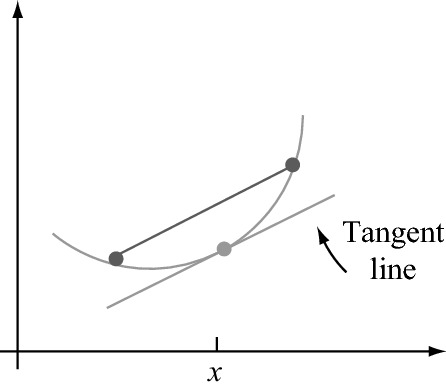
• 158. A function g(x) is convex if the chord connecting any two points on the function’s graph lies above the graph. When g(x) is differentiable, an equivalent condition is that for every x, the tangent line at x lies entirely on or below the graph. (See the accompanying figure.) How does g(μ) = g[E(X)] compare to E[g(X)]? [Hint: The equation of the tangent line at x = μ is y = g(μ) + g′(μ) · (x − μ). Use the condition of convexity, substitute X for x, and take expected values.] Note: Unless g(x) is linear, the resulting inequality, usually called Jensen’s inequality, is strict (< rather than ≤); it is valid for both continuous and discrete rvs.