Separate Your Domains: NIST PQC KEMs, Oracle Cloning and Read-Only Indifferentiability

Abstract

It is convenient and common for schemes in the random oracle model to assume access to multiple random oracles (ROs), leaving to implementations the task—we call it oracle cloning—of constructing them from a single RO. The first part of the paper is a case study of oracle cloning in KEM submissions to the NIST Post-Quantum Cryptography standardization process. We give key-recovery attacks on some submissions arising from mistakes in oracle cloning, and find other submissions using oracle cloning methods whose validity is unclear. Motivated by this, the second part of the paper gives a theoretical treatment of oracle cloning. We give a definition of what is an “oracle cloning method” and what it means for such a method to “work,” in a framework we call read-only indifferentiability, a simple variant of classical indifferentiability that yields security not only for usage in single-stage games but also in multi-stage ones. We formalize domain separation, and specify and study many oracle cloning methods, including common domain-separating ones, giving some general results to justify (prove read-only indifferentiability of) certain classes of methods. We are not only able to validate the oracle cloning methods used in many of the unbroken NIST PQC KEMs, but also able to specify and validate oracle cloning methods that may be useful beyond that.

1 Introduction

Theoretical works giving, and proving secure, schemes in the random oracle (RO) model [11], often, for convenience, assume access to multiple, independent ROs. Implementations, however, like to implement them all via a single hash function like $\mathsf {SHA2}56$ that is assumed to be a RO.

The transition from one RO to many is, in principle, easy. One can use a method suggested by BR [11] and usually called “domain separation.” For example to build three random oracles $H_1,H_2,H_3$ from a single one, H, define

$$\begin{aligned} H_1(x) = H(\langle 1\rangle \Vert x), H_2(x) = H(\langle 2\rangle \Vert x) \text { and }H_3(x) = H(\langle 3\rangle \Vert x) \;, \end{aligned}$$

(1)

where $\langle i\rangle$ is the representation of integer i as a bit-string of some fixed length, say one byte. One might ask if there is justifying theory: a proof that the above “works,” and a definition of what “works” means. A likely response is that it is obvious it works, and theory would be pedantic.

If it were merely a question of the specific domain-separation method of Eq. (1), we’d be inclined to agree. But we have found some good reasons to revisit the question and look into theoretical foundations. They arise from the NIST Post-Quantum Cryptography (PQC) standardization process [35].

We analyzed the KEM submissions. We found attacks, breaking some of them, that arise from incorrect ways of turning one random oracle into many, indicating that the process is error-prone. We found other KEMs where methods other than Eq. (1) were used and whether or not they work is unclear. In some submissions, instantiations for multiple ROs were left unspecified. In others, they differed between the specification and reference implementation.

Domain separation as per Eq. (1) is a method, not a goal. We identify and name the underlying goal, calling it oracle cloning—given one RO, build many, independent ones. (More generally, given m ROs, build $n>m$ ROs.) We give a definition of what is an “oracle cloning method” and what it means for such a method to “work,” in a framework we call read-only indifferentiability, a simple variant of classical indifferentiability [29]. We specify and study many oracle cloning methods, giving some general results to justify (prove read-only indifferentiability of) certain classes of them. The intent is not only to validate as many NIST PQC KEMs as possible (which we do) but to specify and validate methods that will be useful beyond that.

Below we begin by discussing the NIST PQC KEMs and our findings on them, and then turn to our theoretical treatment and results.

NIST PQC KEMs. In late 2016, NIST put out a call for post-quantum cryptographic algorithms [35]. In the first round they received 28 submissions targeting IND-CCA-secure KEMs, of which 17 remain in the second round [37].

Recall that in a KEM (Key Encapsulation Mechanism) ${\mathsf {KE}}$, the encapsulation algorithm $\mathsf {{\mathsf {KE}}{.}E}$ takes the public key (but no message) to return a symmetric key K and a ciphertext $C^*$ encapsulating it, . Given an IND-CCA KEM, one can easily build an IND-CCA PKE scheme by hybrid encryption [18], explaining the focus of standardization on the KEMs.

Most of the KEM submissions (23 in the first round, 15 in the second round) are constructed from a weak (OW-CPA, IND-CPA, ...) PKE scheme using either a method from Hofheinz, Hövelmanns and Kiltz (HHK) [24] or a related method from [21, 27, 40]. This results in a KEM ${\mathsf {KE}}_{4}$, the subscript to indicate that it uses up to four ROs that we’ll denote $H _1, H _2, H _3, H _4$. Results of [21, 24, 27, 40] imply that ${\mathsf {KE}}_{4}$ is provably IND-CCA, assuming the ROs $H _1, H _2, H _3, H _4$ are independent.

Next, the step of interest for us, the oracle cloning: they build the multiple random oracles via a single RO $H$, replacing $H _i$ with an oracle $\mathbf {F}[ H ](i,\cdot )$, where we refer to the construction $\mathbf {F}$ as a “cloning functor,” and $\mathbf {F}[ H ]$ means that $\mathbf {F}$ gets oracle access to $H$. This turns ${\mathsf {KE}}_{4}$ into a KEM ${\mathsf {KE}}_{1}$ that uses only a single RO $H$, allowing an implementation to instantiate the latter with a single NIST-recommended primitive like $\mathsf {SHA3}\text {-}\mathsf {512}$ or $\mathsf {SHAKE256}$ [36]. (In some cases, ${\mathsf {KE}}_{1}$ uses a number of ROs that is more than one but less than the number used by ${\mathsf {KE}}_{4}$, which is still oracle cloning, but we’ll ignore this for now.)

Often the oracle cloning method (cloning functor) is not specified in the submission document; we obtained it from the reference implementation. Our concern is the security of this method and the security of the final, single-RO-using KEM ${\mathsf {KE}}_{1}$. (As above we assume the starting ${\mathsf {KE}}_{4}$ is secure if its four ROs are independent.)

Oracle cloning in submissions. We surveyed the relevant (first- and second-round) NIST PQC KEM submissions, looking in particular at the reference code, to determine what choices of cloning functor $\mathbf {F}$ was made, and how it impacted security of ${\mathsf {KE}}_{1}$. Based on our findings, we classify the submissions into groups as follows.

First is a group of successfully attacked submissions. We discover and specify attacks, enabled through erroneous RO cloning, on three (first-round) submissions:    [8],    [7] and    [22]. (Throughout the paper, first-round submissions are in   , second-round submissions in .) Our attacks on   and   recover the symmetric key K from the ciphertext $C^*$ and public key. Our attack on   succeeds in partial key recovery, recovering 192 bits of the symmetric key. These attacks are very fast, taking at most about the same time as taken by the (secret-key equipped, prescribed) decryption algorithm to recover the key. None of our attacks needs access to a decryption oracle, meaning we violate much more than IND-CCA.

Next is submissions with questionable oracle cloning. We put just one in this group, namely    [2]. Here we do not have proof of security in the ROM for the final instantiated scheme ${\mathsf {KE}}_{1}$. We do show that the cloning methods used here do not achieve our formal notion of rd-indiff security, but this does not result in an attack on ${\mathsf {KE}}_{1}$, so we do not have a practical attack either. We recommend changes in the cloning methods that permit proofs.

Next is a group of ten submissions that use ad-hoc oracle cloning methods—as opposed, say, to conventional domain separation as per Eq. (1)—but for which our results (to be discussed below) are able to prove security of the final single-RO scheme. In this group are    [3],    [44],    [28],    [16],    [4],    [38],    [30],    [6],    [19] and    [43]. Still, the security of these oracle cloning methods remains brittle and prone to vulnerabilities under slight changes.

A final group of twelve submissions did well, employing something like Eq. (1). In particular our results can prove these methods secure. In this group are    [13],    [5],    [41],    [34],    [32],    [42],    [25],    [14],    [1],    [31],    [26] and  [23].

This classification omits 14 KEM schemes that do not fit the above framework. (For example they do not target IND-CCA KEMs, do not use HHK-style transforms, or do not use multiple random oracles.)

Lessons and response. We see that oracle cloning is error-prone, and that it is sometimes done in ad-hoc ways whose validity is not clear. We suggest that oracle cloning not be left to implementations. Rather, scheme designers should give proof-validated oracle cloning methods for their schemes. To enable this, we initiate a theoretical treatment of oracle cloning. We formalize oracle cloning methods, define what it means for one to be secure, and specify a library of proven-secure methods from which designers can draw. We are able to justify the oracle cloning methods of many of the unbroken NIST PQC KEMs. The framework of read-only indifferentiability we introduce and use for this purpose may be of independent interest.

The NIST PQC KEMs we break are first-round candidates, not second-round ones, and in some cases other attacks on the same candidates exist, so one may say the breaks are no longer interesting. We suggest reasons they are. Their value is illustrative, showing not only that errors in oracle cloning occur in practice, but that they can be devastating for security. In particular, the extensive and long review process for the first-round NIST PQC submissions seems to have missed these simple attacks, perhaps due to lack of recognition of the importance of good oracle cloning.

Indifferentiability background. Let $\mathsf {SS},\mathsf {ES}$ be sets of functions. (We will call them the starting and ending function spaces, respectively.) A functor $\mathbf {F} {:\;\;}\mathsf {SS} \rightarrow \mathsf {ES}$ is a deterministic algorithm that, given as oracle a function $s \in \mathsf {SS}$, defines a function $\mathbf {F}[ s ] \in \mathsf {ES}$. Indifferentiability of $\mathbf {F}$ is a way of defining what it means for $\mathbf {F}[ s ]$ to emulate $e$ when $s , e$ are randomly chosen from $\mathsf {SS},\mathsf {ES}$, respectively. It permits a “composition theorem” saying that if $\mathbf {F}$ is indifferentiable then use of $e$ in a scheme can be securely replaced by use of $\mathbf {F}[ s ]$.

Maurer, Renner and Holenstein (MRH) [29] gave the first definition of indifferentiability and corresponding composition theorem. However, Ristenpart, Shacham and Shrimpton (RSS) [39] pointed out a limitation, namely that it only applies to single-stage games. MRH-indiff fails to guarantee security in multi-stage games, a setting that includes many goals of interest including security under related-key attack, deterministic public-key encryption and encryption of key-dependent messages. Variants of MRH-indiff [17, 20, 33, 39] tried to address this, with limited success.

Rd-indiff. Indifferentiability is the natural way to treat oracle cloning. A cloning of one function into n functions ($n=4$ above) can be captured as a functor (we call it a cloning functor) $\mathbf {F}$ that takes the single RO $s$ and for each $i \in [1..n]$ defines a function $\mathbf {F}[ s ](i,\cdot )$ that is meant to emulate a RO. We will specify many oracle cloning methods in this way.

We define in Sect. 4 a variant of indifferentiability we call read-only indifferentiability (rd-indiff). The simulator—unlike for reset-indiff [39]—has access to a game-maintained state $st$, but—unlike MRH-indiff [29]—that state is read-only, meaning the simulator cannot alter it across invocations. Rd-indiff is a stronger requirement than MRH-indiff (if $\mathbf {F}$ is rd-indiff then it is MRH-indiff) but a weaker one than reset-indiff (if $\mathbf {F}$ is reset-indiff then it is rd-indiff). Despite the latter, rd-indiff, like reset-indiff, admits a composition theorem showing that an rd-indiff $\mathbf {F}$ may securely substitute a RO even in multi-stage games. (The proof of RSS [39] for reset-indiff extends to show this.) We do not use reset-indiff because some of our cloning functors do not meet it, but they do meet rd-indiff, and the composition benefit is preserved.

General results. In Sect. 4, we define translating functors. These are simply ones whose oracle queries are non-adaptive. (In more detail, a translating functor determines from its input W a list of queries, makes them to its oracle and, from the responses and W, determines its output.) We then define a condition on a translating functor $\mathbf {F}$ that we call invertibility and show that if $\mathbf {F}$ is an invertible translating functor then it is rd-indiff. This is done in two parts, Theorems 1 and 2, that differ in the degree of invertibility assumed. The first, assuming the greater degree of invertibility, allows a simpler proof with a simulator that does not need the read-only state allowed in rd-indiff. The second, assuming the lesser degree of invertibility, depends on a simulator that makes crucial use of the read-only state. It sets the latter to a key for a PRF that is then used to answer queries that fall outside the set of ones that can be trivially answered under the invertibility condition. This use of a computational primitive (a PRF) in the indifferentiability context may be novel and may seem odd, but it works.

We apply this framework to analyze particular, practical cloning functors, showing that these are translating and invertible, and then deducing their rd-indiff security. But the above-mentioned results are stronger and more general than we need for the application to oracle cloning. The intent is to enable further, future applications.

Analysis of oracle cloning methods. We formalize oracle cloning as the task of designing a functor (we call it a cloning functor) $\mathbf {F}$ that takes as oracle a function $s\in \mathsf {SS}$ in the starting space and returns a two-input function $e= \mathbf {F}[s] \in \mathsf {ES}$, where $e(i,\cdot )$ represents the i-th RO for $i\in [1..n]$. Section 5 presents the cloning functors corresponding to some popular and practical oracle cloning methods (in particular ones used in the NIST PQC KEMs), and shows that they are translating and invertible. Our above-mentioned results allow us to then deduce they are rd-indiff, which means they are safe to use in most applications, even ones involving multi-stage games. This gives formal justification for some common oracle cloning methods. We now discuss some specific cloning functors that we treat in this way.

The prefix (cloning) functor $\mathbf {F}_{\mathrm {pf}(\mathbf {p})}$ is parameterized by a fixed, public vector $\mathbf {p}$ such that no entry of $\mathbf {p}$ is a prefix of any other entry of $\mathbf {p}$. Receiving function $s$ as an oracle, it defines function $e= \mathbf {F}_{\mathrm {pf}(\mathbf {p})}[ s ]$ by $e(i,X) = s (\mathbf {p}[i]\Vert X)$, where $\mathbf {p}[i]$ is the $i^{\text {th}}$ element of vector $\mathbf {p}$. When $\mathbf {p}[i]$ is a fixed-length bitstring representing the integer i, this formalizes Eq. (1).

Some NIST PQC submissions use a method we call output splitting. The simplest case is that we want $e(i,\cdot ),\ldots ,{\epsilon }(n,\cdot )$ to all have the same output length L. We then define e(i, X) as bits $(i-1)L\,+\,1$ through iL of the given function $s$ applied to X. That is, receiving function $s$ as an oracle, the splitting (cloning) functor $\mathbf {F}_{\mathrm {spl}}$ returns function $e= \mathbf {F}_{\mathrm {spl}}[ s ]$ defined by $e(i,X) = s(X)[(i-1)L\!+\!1 .. iL]$.

An interesting case, present in some NIST PQC submissions, is trivial cloning: just set $e(i,X)=s(X)$ for all X. We formalize this as the identity (cloning) functor $\mathbf {F}_{\mathrm {id}}$ defined by $\mathbf {F}_{\mathrm {id}}[s](i,X) = s(X)$. Clearly, this is not always secure. It can be secure, however, for usages that restrict queries in some way. One such restriction, used in several NIST PQC KEMs, is length differentiation: $e(i,\cdot )$ is queried only on inputs of some length $l_i$, where $l_1,\ldots ,l_n$ are chosen to be distinct. We are able to treat this in our framework using the concept of working domains that we discuss next, but we warn that this method is brittle and prone to misuse.

Working domains. One could capture trivial cloning with length differentiation as a restriction on the domains of the ending functions, but this seems artificial and dangerous because the implementations do not enforce any such restriction; the functions there are defined on their full domains and it is, apparently, left up to applications to use the functions in a way that does not get them into trouble. The approach we take is to leave the functions defined on their full domains, but define and ask for security over a subdomain, which we called the working domain. A choice of working domain $\mathcal{W}$ accordingly parameterizes our definition of rd-indiff for a functor, and also the definition of invertibility of a translating functor. Our result says that the identity functor is rd-indiff for certain choices of working domains that include the length differentiation one.

Making the working domain explicit will, hopefully, force the application designer to think about, and specify, what it is, increasing the possibility of staying out of trouble. Working domains also provide flexibility and versatility under which different applications can make different choices of the domain.

Working domains not being present in prior indifferentiability formalizations, the comparisons, above, of rd-indiff with these prior formalizations assume the working domain is the full domain of the ending functions. Working domains alter the comparison picture; a cloning functor which is rd-indiff on a working domain may not be even MRH-indiff on its full domain.

Application to KEMs. The framework above is broad, staying in the land of ROs and not speaking of the usage of these ROs in any particular cryptographic primitive or scheme. As such, it can be applied to analyze RO instantiation in many primitives and schemes. In the full version of this paper [10], we exemplify its application in the realm of KEMs as the target of the NIST PQC designs.

This may seem redundant, since an indifferentiability composition theorem says exactly that once indifferentiability of a functor has been shown, “all” uses of it are secure. However, prior indifferentiability frameworks do not consider working domains, so the known composition theorems apply only when the working domain is the full one. (Thus the reset-indiff composition theorem of [39] extends to rd-indiff so that we have security for applications whose security definitions are underlain by either single or multi-stage games, but only for full working domains.)

To give a composition theorem that is conscious of working domains, we must first ask what they are, or mean, in the application. We give a definition of the working domain of a KEM ${\mathsf {KE}}$ . This is the set of all points that the scheme algorithms query to the ending functions in usage, captured by a certain game we give. (Queries of the adversary may fall outside the working domain.) Then we give a working-domain-conscious composition theorem for KEMs that says the following. Say we are given an IND-CCA KEM ${\mathsf {KE}}$ whose oracles are drawn from a function space $\mathsf {{\mathsf {KE}}{.}FS}$. Let $\mathbf {F}{:\;\;}\mathsf {SS} \rightarrow \mathsf {{\mathsf {KE}}{.}FS}$ be a functor, and let $\overline{\mathsf {KE}}$ be the KEM obtained by implementing the oracles of the ${\mathsf {KE}}$ via $\mathbf {F}$. (So the oracles of this second KEM are drawn from the function space $\mathsf {\overline{\mathsf {KE}}{.}FS}= \mathsf {SS}$.) Let $\mathcal{W}$ be the working domain of ${\mathsf {KE}}$, and assume $\mathbf {F}$ is rd-indiff over $\mathcal{W}$. Then $\overline{\mathsf {KE}}$ is also IND-CCA. Combining this with our rd-indiff results on particular cloning functors justifies not only conventional domain separation as an instantiation technique for KEMs, but also more broadly the instantiations in some NIST PQC submissions that do not use domain separation, yet whose cloning functors are rd-diff over the working domain of their KEMs. The most important example is the identity cloning functor used with length differentiation.

A key definitional element of our treatment that allows the above is, following [9], to embellish the syntax of a scheme (here a KEM ${\mathsf {KE}}$) by having it name a function space $\mathsf {{\mathsf {KE}}{.}FS}$ from which it wants its oracles drawn. Thus, the scheme specification must say how many ROs it wants, and of what domains and ranges. In contrast, in the formal version of the ROM in [11], there is a single, scheme-independent RO that has some fixed domain and range, for example mapping $\{0,1\}^*$ to $\{0,1\}$. This leaves a gap, between the object a scheme wants and what the model provides, that can lead to error. We suggest that, to reduce such errors, schemes specified in standards include a specification of their function space.

2 Oracle Cloning in NIST PQC Candidates

Notation. A KEM scheme ${\mathsf {KE}}$ specifies an encapsulation $\mathsf {{\mathsf {KE}}{.}E}$ that, on input a public encryption key returns a session key K, and a ciphertext $C^*$ encapsulating it, written . A PKE scheme ${\mathsf {PKE}}$ specifies an encryption algorithm $\mathsf {{\mathsf {PKE}}{.}E}$ that, on input , message $M\in \{0,1\}^{\mathsf {{\mathsf {PKE}}{.}ml}}$ and randomness R, deterministically returns ciphertext . For neither primitive will we, in this section, be concerned with the key generation or decapsulation/decryption algorithm. We might write ${\mathsf {KE}}[X_1,X_2,\ldots ]$ to indicate that the scheme has oracle access to functions $X_1,X_2,\ldots$, and correspondingly then write $\mathsf {{\mathsf {KE}}{.}E}[X_1,X_2,\ldots ]$, and similarly for ${\mathsf {PKE}}$.

2.1 Design Process

The literature [21, 24, 27, 40] provides many transforms that take a public-key encryption scheme ${\mathsf {PKE}}$, assumed to meet some weaker-than-IND-CCA notion of security we denote $\mathrm {S}_{\mathrm {pke}}$ (for example, OW-CPA, OW-PCA or IND-CPA), and, with the aid of some number of random oracles, turn ${\mathsf {PKE}}$ into a KEM that is guaranteed (proven) to be IND-CCA assuming the ROs are independent. We’ll refer to such transforms as sound. Many (most) KEMs submitted to the NIST Post-Quantum Cryptography standardization process were accordingly designed as follows:

• (1) First, they specify a $\mathrm {S}_{\mathrm {pke}}$-secure public-key encryption scheme ${\mathsf {PKE}}$.

• (2) Second, they pick a sound transform $\mathbf {T}$ and obtain KEM ${\mathsf {KE}}_{4}[ H _1, H _2, H _3, H _4] = \mathbf {T}[{\mathsf {PKE}}, H _2, H _3, H _4]$. (The notation is from [24]. The transforms use up to three random oracles that we are denoting $H _2, H _3, H _4$, reserving $H _1$ for possible use by the PKE scheme.) We refer to ${\mathsf {KE}}_{4}$ (the subscript refers to its using 4 oracles) as the base KEM, and, as we will see, it differs across the transforms.

• (3) Finally—the under-the-radar step that is our concern—the ROs $H _1,\ldots , H _4$ are constructed from cryptographic hash functions to yield what we call the final KEM ${\mathsf {KE}}_{1}$. In more detail, the submissions make various choices of cryptographic hash functions $F _1,\ldots , F _m$ that we call the base functions, and, for $i=1,2,3,4$, specify constructions $\mathbf {C}_i$ that, with oracle access to the base functions, define the $H _i$, which we write as $H _i \leftarrow \mathbf {C}_i[ F _1,\ldots , F _m]$. We call this process oracle cloning, and we call $H_i$ the final functions. (Common values of m are 1, 2.) The actual, submitted KEM ${\mathsf {KE}}_{1}$ (the subscript because m is usually 1) uses the final functions, so that its encapsulation algorithm can be written as:

  

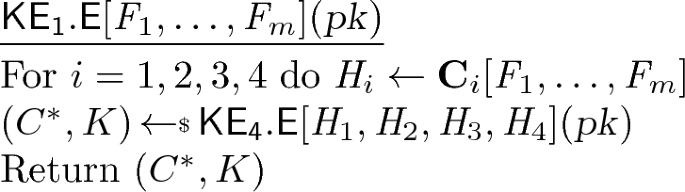
The question now is whether the final ${\mathsf {KE}}_{1}$ is secure. We will show that, for some submissions, it is not. This is true for the choices of base functions $F _1,\ldots , F _m$ made in the submission, but also if these are assumed to be ROs. It is true despite the soundness of the transform, meaning insecurity arises from poor oracle cloning, meaning choices of the constructions $\mathbf {C}_i$. We will then consider submissions for which we have not found an attack. In the latter analysis, we are willing to assume (as the submissions implicitly do) that $F _1,\ldots , F _m$ are ROs, and we then ask whether the final functions are “close” to independent ROs.

Fig. 1.

Top: Encapsulation algorithm of the base KEM scheme produced by our parameterized transform. Bottom: Choices of parameters $X,Y,Z,\mathsf {D},\mathsf {k}^*$ resulting in specific transforms used by the NIST PQC submissions. Second-round submissions are in , first-round submissions in   . Submissions using different transforms in the two rounds appear twice.

2.2 The Base KEM

We need first to specify the base ${\mathsf {KE}}_{4}$ (the result of the sound transform, from step (2) above). The NIST PQC submissions typically cite one of HHK [24], Dent [21], SXY [40] or JZCWM [27] for the sound transform they use, but our examinations show that the submissions have embellished, combined or modified the original transforms. The changes do not (to best of our knowledge) violate soundness (meaning the used transforms still yield an IND-CCA ${\mathsf {KE}}_{4}$ if $H _2, H _3, H _4$ are independent ROs and ${\mathsf {PKE}}$ is $\mathrm {S}_{\mathrm {pke}}$-secure) but they make a succinct exposition challenging. We address this with a framework to unify the designs via a single, but parameterized, transform, capturing the submission transforms by different parameter choices.

Figure 1 (top) shows the encapsulation algorithm $\mathsf {{\mathsf {KE}}_{4}{.}E}$ of the KEM that our parameterized transform associates to ${\mathsf {PKE}}$ and $H_1,H_2,H_3,H_4$. The parameters are the variables X, Y, Z (they will be functions of other quantities in the algorithms), a boolean $\mathsf {D}$, and an integer $\mathsf {k}^*$. When choices of these are made, one gets a fully-specified transform and corresponding base KEM ${\mathsf {KE}}_{4}$. Each row in the table in the same Figure shows one such choice of parameters, resulting in 15 fully-specified transforms. The final column shows the submissions that use the transform.

The encapsulation algorithm at the top of Fig. 1 takes input a public key and has oracle access to functions $H_1,H_2,H_3,H_4$. At line 1, it picks a random seed M of length the message length of the given PKE scheme. Boolean $\mathsf {D}$ being $\mathsf {true}$ (as it is with just one exception) means $\mathsf {{\mathsf {PKE}}{.}E}$ is randomized. In that case, line 2 applies $H_2$ to X (the latter, determined as per the table, depends on M and possibly also on ) and parses the output to get coins R for $\mathsf {{\mathsf {PKE}}{.}E}$ and possibly (if the parameter $\mathsf {k}^*\ne 0$) an additional string $K'$. At line 3, a ciphertext $C$ is produced by encrypting the seed M using $\mathsf {{\mathsf {PKE}}{.}E}$ with public key and coins R. In some schemes, a second portion of the ciphertext, Y, often called the “confirmation", is derived from X or M, using $H _3$, as shown in the table, and line 4 then defines $C^*$. Finally, $H _4$ is used as a key derivation function to extract a symmetric key K from the parameter Z, which varies widely among transforms.

In total, 26 of the 39 NIST PQC submissions which target KEMs in either the first or second round use transforms which fall into our framework. The remaining schemes do not use more than one random oracle, construct KEMs without transforming PKE schemes, or target security definitions other than IND-CCA.

2.3 Submissions We Break

We present attacks on    [8],    [7], and    [22]. These attacks succeed in full or partial recovery of the encapsulated KEM key from a ciphertext, and are extremely fast. We have implemented the attacks to verify them.

Although none of these schemes progressed to Round 2 of the competition without significant modification, to the best of our knowledge, none of the attacks we described were pointed out during the review process. Given the attacks’ superficiality, this is surprising and suggests to us that more attention should be paid to oracle cloning methods and their vulnerabilities during review.

Randomness-based decryption. The PKE schemes used by and have the property that given a ciphertext and also given the coins R, it is easy to recover M, even without knowledge of the secret key. We formalize this property, saying ${\mathsf {PKE}}$ allows randomness-based decryption, if there is an (efficient) algorithm $\mathsf {{\mathsf {PKE}}{.}DecR}$ such that for any public key , coins R and message m. This will be used in our attacks.

Attack on . The base KEM ${\mathsf {KE}}_1[H_1,H_2,H_3,H_4]$ is given by the transform $\mathbf {T}_9$ in the table of Fig. 1. The final KEM ${\mathsf {KE}}_2[F]$ uses a single function F to instantiate the random oracles, which it does as follows. It sets $H_3=H_4=F$ and $H_2=W[F]\,\circ \,F$ for a certain function W (the rejection sampling algorithm) whose details will not matter for us. The notation W[F] meaning that W has oracle access to F. The following attack (explanations after the pseudocode) recovers the encapsulated KEM key K from ciphertext —

As per $\mathbf {T}_9$ we have $Y = H_3(M) = F(M)$. The coins for $\mathsf {{\mathsf {PKE}}{.}E}$ are $R = H_2(M) = (W[F]\circ F)(M) = W[F](F(M)) = W[F](Y)$. Since Y is in the ciphertext, the coins R can be recovered as shown at line 2. The PKE scheme allows randomness-based decryption, so at line 3 we can recover the message M underlying C using algorithm $\mathsf {{\mathsf {PKE}}{.}DecR}$. But $K = H_4(M) = F(M)$, so K can now be recovered as well. In conclusion, the specific cloning method chosen by leads to complete recovery of the encapsulated key from the ciphertext.

Attack on . The base KEM ${\mathsf {KE}}_1[H_2,H_3,H_4]$ is given by the transform $\mathbf {T}_{11}$ in the table of Fig. 1. The final KEM ${\mathsf {KE}}_2[F]$ uses a single base function F to instantiate the final functions, which it does as follows. It sets $H_4=F$. The specification and reference implementation differ in how $H_2,H_3$ are defined: In the former, $H _2(x) = F(F(x)){\,\Vert \,}F(x)$ and $H _3(x) = F(F(F(x)))$, while, in the latter, $H _2(x) = F(F(F(x))) {\,\Vert \,}F(x)$ and $H _3(x) = F(F(X))$. These differences arise from differences in the way the output of a certain function W[F] is parsed.

Our attack is on the reference-implementation version of the scheme. We need to also know that the scheme sets $\mathsf {k}^*$ so that $R\Vert K'\leftarrow H_2(X)$ with $H_2(X) = F(F(F(X)))\Vert F(X)$ results in $R = F(F(F(X)))$. But $Y=H_3(X) = F(F(X))$, so $R=F(Y)$ can be recovered from the ciphertext. Again exploiting the fact that the PKE scheme allows randomness-based decryption, we obtain the following attack that recovers the encapsulated KEM key K from ciphertext —

This attack exploits the difference between the way $H_2,H_3$ are defined across the specification and implementation, which may be a bug in the implementation with regard to the parsing of W[F](x). However, the attack also exploits dependencies between $H _2$ and $H _3$, which ought not to exist when instantiating what are required to be distinct random oracles.

  was incorporated into the second-round submission   , which specifies a different base function and cloning functor (the latter of which uses the secure method we call “output splitting”) to instantiate oracles $H_2$ and $H_3$. This attack therefore does not apply to .

Attack on DAGS. If x is a byte string we let x[i] be its i-th byte, and if x is a bit string we let $x_i$ be its i-th bit. We say that a function V is an extendable output function if it takes input a string x and an integer $\ell$ to return an $\ell$-byte output, and $\ell _1 \le \ell _2$ implies that $V(x,\ell _1)$ is a prefix of $V(x,\ell _2)$. If $v = v_1v_2v_3v_4v_5v_6v_7v_8$ is a byte then let $Z(v) = 00v_3v_4v_5v_6v_7v_8$ be obtained by zeroing out the first two bits. If y is a string of $\ell$ bytes then let $Z'(y) = Z(y[1])\Vert \cdots \Vert Z(y[\ell ])$. Now let $V'(x,\ell ) = Z'(V(x,\ell ))$.

The base KEM ${\mathsf {KE}}_1[H_1,H_2,H_3,H_4]$ is given by the transform $\mathbf {T}_{8}$ in the table of Fig. 1. The final KEM ${\mathsf {KE}}_2[V]$ uses an extendable output function V to instantiate the random oracles, which it does as follows. It sets $H _2(x) = V'(x,512)$ and $H _3(x) = V'(x,32)$. It sets $H _4(x) = V(x,64)$.

As per $\mathbf {T}_8$ we have $K = H_4(M)$ and $Y = H_3(M)$. Let L be the first 32 bytes of the 64-byte K. Then $Y = Z'(L)$. So Y reveals $32\cdot 6 = 192$ bits of K. Since Y is in the ciphertext, this results in a partial encapsulated-key recovery attack. The attack reduces the effective length of K from $64\cdot 8 = 512$ bits to $512-192 = 320$ bits, meaning $37.5\%$ of the encapsulated key is recovered. Also $R = H_2(M)$, so Y, as part of the ciphertext, reveals 32 bytes of R, which does not seem desirable, even though it is not clear how to exploit it for an attack.

2.4 Submissions with Unclear Security

For the scheme  [2], we can give neither an attack nor a proof of security. However, we can show that the final functions $H_2, H_3, H_4$ produced by the cloning functor with oracle access to a single extendable-output function V are differentiable from independent random oracles. The cloning functor sets $H_1(x)=V(x,128)$ and $H_4 = V(x,32)$. It computes $H_2$ and $H_3$ from V using the output splitting cloning functor. Concretely, ${\mathsf {KE}}_2$ parses V(x, 96) as $H_2(x){\,\Vert \,}H_3(x)$, where $H_2$ has output length 64 bytes and $H_3$ has output length 32 bytes. Because V is an extendable-output function, $H_4(x)$ will be a prefix of $H_2(x)$ for any string x.

We do not know how to exploit this correlation to attack the IND-CCA security of the final KEM scheme ${\mathsf {KE}}_2[V]$, and we conjecture that, due to the structure of $\mathbf {T}_{10}$, no efficient attack exists. We can, however, attack the rd-indiff security of functor , showing that that the security proof for the base KEM ${\mathsf {KE}}_1[H_2,H_3,H_4]$ does not naturally transfer to ${\mathsf {KE}}_2[V]$. Therefore, in order to generically extend the provable security results for ${\mathsf {KE}}_1$ to ${\mathsf {KE}}_2$, it seems advisable to instead apply appropriate oracle cloning methods.

2.5 Submissions with Provable Security but Ambiguous Specification

In their reference implementations, these submissions use cloning functors which we can and do validate via our framework, providing provable security in the random oracle model for the final KEM schemes. However, the submission documents do not clearly specify a secure cloning functor, meaning that variant implementations or adaptations may unknowingly introduce weaknesses. The schemes    [3],    [44],    [28],    [16],    [4],    [38],    [30],    [6],    [19] and    [43] fall into this group.

Length differentiation. Many of these schemes use the “identity” functor in their reference implementations, meaning that they set the final functions $H_1 = H_2 = H_3 = H_4 = F$ for a single base function F. If the scheme ${\mathsf {KE}}_1[H_1,H_2,H_3,H_4]$ never queries two different oracles on inputs of a single length, the domains of $H_1,\ldots ,H_4$ are implicitly separated. Reference implementations typically enforce this separation by fixing the input length of every call to F. Our formalism calls this query restriction “length differentiation” and proves its security as an oracle cloning method. We also generalize it to all methods which prevent the scheme from querying any two distinct random oracles on a single input.

In the following, we discuss two schemes from the group, and , where ambiguity about cloning methods between the specification and reference implementation jeopardizes the security of applications using these schemes. It will be important that, like and , the PKE schemes defined by and allow randomness-based decryption.

The scheme [30] defines its base KEM ${\mathsf {KE}}_1[H_1,H_2,H_3,H_4]$ using the $\mathbf {T}_9$ transform from Fig. 1. The submission document states that $H _1$, $H _2$, $H _3$, and $H _4$ are “typically” instantiated with a single fixed-length hash function F, but does not describe the cloning functors used to do so. If the identity functor is used, so that $H_1 = H_2 = H_3 = H_4 = F$, (or more generally, any functor that sets $H_2=H_3$), an attack is possible. In the transform $\mathbf {T}_9$, both $H _2$ and $H _3$ are queried on the same input M. Then $Y = H_3(M) = F(M) = H_2(M) = R$ leaks the PKE’s random coins, so the following attack will allow total key recovery via the randomness-based decryption.

In the reference implementation of , however, $H _2$ is instantiated using a second, independent function V instead of F, which prevents the above attack. Although the random oracles $H_1,H_3$ and $H_4$ are instantiated using the identity functor, they are never queried on the same input thanks to length differentiation. As a result, the reference implementation of is provably secure, though alternate implementations could be both compliant with the submission document and completely insecure. The relevant portions of both the specification and the reference implementation were originally found in the corresponding first-round submission ( ).

  [16] also follows transform $\mathbf {T}_9$ to produce its base KEM ${\mathsf {KE}}_1[H_2,H_3,H_4]$. Its submission document suggests instantiation with a single function F as follows: it sets $H_3 = H_4 = F$, and it sets $H_2 = W \circ F$ for some postprocessing function W whose details are irrelevant here. Since, in $\mathbf {T}_9$, $Y = H _3(M) = F(M)$ and $R = H _2(M) = W\circ F (M) = W(Y)$, the randomness R will again be leaked through Y in the ciphertext, permitting a key-recovery attack using randomness-based decryption much like the others we have described. This attack is prevented in the reference implementation of   , which instantiates $H_3$ and $H_4$ using an independent function G. The domains of $H_3$ and $H_4$ are separated by length differentiation. This allows us to prove the security of the final KEM ${\mathsf {KE}}_2[G,F]$, as defined by the reference implementation.

However, the length differentiation of $H _3$ and $H _4$ breaks down in the chosen-ciphertext-secure PKE variant specification of   , which transforms ${\mathsf {KE}}_1$. The PKE scheme, given a plaintext M, computes $R=H_2(M)$ and $Y=H_3(M)$ according to $\mathbf {T}_9$, but it computes $K = H_4(M)$, then includes the value $B = K \oplus M$ as part of the ciphertext $C^*$. Both the identity functor and the functor used by the KEM reference implementation set $H_3 = H_4$, so the following attack will extract the plaintext from any ciphertext–

The reference implementation of the public-key encryption schemes prevents the attack by cloning $H _3$ and $H _4$ from G via a third cloning functor, this one using the output splitting method. Yet, the inconsistency in the choice of cloning functors between the specification and both implementations underlines that ad-hoc cloning functors may easily “get lost” in modifications or adaptations of a scheme.

2.6 Submissions with Clear Provable Security

Here we place schemes which explicitly discuss their methods for domain separation and follow good practice in their implementations:    [13],    [5],    [41],    [34],    [32],    [42],    [25],    [14],    [1],    [31],    [26] and    [23]. These schemes are careful to account for dependencies between random oracles that are considered to be independent in their security models. When choosing to clone multiple random oracles from a single primitive, the schemes in this group use padding bytes, deploy hash functions designed to accommodate domain separation, or restrictions on the length of the inputs which are codified in the specification. These explicit domain separation techniques can be cast in the formalism we develop in this work.

  and are unique among the PQC KEM schemes in that their specifications warn that the identity functor admits key-recovery attacks. As protection, they recommend that $H _2$ and $H _3$ be instantiated with unrelated primitives.

Signatures. Although the main focus of this paper is on domain separation in KEMs, we wish to note that these issues are not unique to KEMs. At least one digital signature scheme in the second round of the NIST PQC competition,  [15], models multiple hash functions as independent random oracles in its security proof, then clones them from the same primitive without explicit domain separation. We have not analyzed the NIST PQC digital signature schemes’ security to see whether more subtle domain separation is present, or whether oracle collisions admit the same vulnerabilities to signature forgery as they do to session key recovery. This does, however, highlight that the problem of random oracle cloning is pervasive among more types of cryptographic schemes.

3 Preliminaries

Basic notation. By [i..j] we abbreviate the set $\{i,\ldots ,j\}$, for integers $i \le j$. If $\mathbf {x}$ is a vector then $|\mathbf {x}|$ is its length (the number of its coordinates), $\mathbf {x}[i]$ is its i-th coordinate and $[\mathbf {x}]=\{\mathbf {x}[i] \,:\, i\in [1..|\mathbf {x}|]\}$ is the set of its coordinates. The empty vector is denoted (). If S is a set, then $S^*$ is the set of vectors over S, meaning the set of vectors of any (finite) length with coordinates in S. Strings are identified with vectors over $\{0,1\}$, so that if $x \in \{0,1\}^*$ is a string then |x| is its length, x[i] is its i-th bit, and x[i..j] is the substring from its i-th to its j-th bit (including), for $i \le j$. The empty string is $\varepsilon$. If x, y are strings then we write $x \preceq y$ to indicate that x is a prefix of y. If S is a finite set then |S| is its size (cardinality). A set $S\subseteq \{0,1\}^*$ is length closed if $\{0,1\}^{|x|}\subseteq S$ for all $x\in S$.

We let $y \leftarrow A[\mathsf {O}_1, \ldots ](x_1,\ldots ; r)$ denote executing algorithm A on inputs $x_1,\ldots$ and coins r, with access to oracles $\mathsf {O}_1, \ldots$, and letting y be the result. We let be the resulting of picking r at random and letting $y \leftarrow A[\mathsf {O}_1, \ldots ](x_1,\ldots ;r)$. We let $\mathrm {OUT}(A[\mathsf {O}_1, \ldots ](x_1,\ldots ))$ denote the set of all possible outputs of algorithm A when invoked with inputs $x_1,\ldots$ and access to oracles $\mathsf {O}_1, \ldots$. Algorithms are randomized unless otherwise indicated. Running time is worst case. An adversary is an algorithm.

We use the code-based game-playing framework of [12]. A game $\text {G}$ (see Fig. 2 for an example) starts with an $\textsc {init}$ procedure, followed by a non-negative number of additional procedures, and ends with a $\textsc {fin}$ procedure. Procedures are also called oracles. Execution of adversary $\mathcal {A}$ with game $\text {G}$ consists of running $\mathcal {A}$ with oracle access to the game procedures, with the restrictions that $\mathcal {A}$’s first call must be to $\textsc {init}$, its last call must be to $\textsc {fin}$, and it can call these two procedures at most once. The output of the execution is the output of $\textsc {fin}$. We write $\Pr [\text {G}(\mathcal {A})]$ to denote the probability that the execution of game $\text {G}$ with adversary $\mathcal {A}$ results in the output being the boolean $\mathsf {true}$. Note that our adversaries have no output. The role of what in other treatments is the adversary output is, for us, played by the query to $\textsc {fin}$. We adopt the convention that the running time of an adversary is the worst-case time to execute the game with the adversary, so the time taken by game procedures (oracles) to respond to queries is included.

Functions. As usual $g{:\;\;}\mathcal {D}\rightarrow \mathcal {R}$ indicates that g is a function taking inputs in the domain set $\mathcal {D}$ and returning outputs in the range set $\mathcal {R}$. We may denote these sets by $\mathrm {Dom}({g})$ and $\mathrm {Rng}({g})$, respectively.

We say that $g{:\;\;}\mathrm {Dom}({g}) \rightarrow \mathrm {Rng}({g})$ has output length $\ell$ if $\mathrm {Rng}({g})=\{0,1\}^{\ell }$. We say that g is a single output-length (sol) function if there is some $\ell$ such that g has output length $\ell$ and also the set $\mathcal {D}$ is length closed. We let $\mathrm {SOL}(\mathcal {D},\ell )$ denote the set of all sol functions $g{:\;\;}\mathcal {D}\rightarrow \{0,1\}^{\ell }$.

We say g is an extendable output length (xol) function if the following are true: (1) $\mathrm {Rng}({g})=\{0,1\}^*$ (2) there is a length-closed set $\mathrm {Dom}_{*}({g})$ such that $\mathrm {Dom}({g}) = \mathrm {Dom}_{*}({g}) \times {{\mathbb N}}$ (3) $|g(x,\ell )|=\ell$ for all $(x,\ell )\in \mathrm {Dom}({g})$, and (4) $g(x,\ell )\preceq g(x,\ell ')$ whenever $\ell \le \ell '$. We let $\mathrm {XOL}(\mathcal {D})$ denote the set of all xol functions $g{:\;\;}\mathcal {D}\rightarrow \{0,1\}^{*}$.

4 Read-Only Indifferentiability of Translating Functors

We define read-only indifferentiability (rd-indff) of functors. Then we define a class of functors called translating, and give general results about their rd-indiff security. Later we will apply this to analyze the security of cloning functors, but the treatment in this section is broader and, looking ahead to possible future applications, more general than we need for ours.

4.1 Functors and Read-Only Indifferentiability

A random oracle, formally, is a function drawn at random from a certain space of functions. A construction (functor) is a mapping from one such space to another. We start with definitions for these.

Function spaces and functors. A function space $\mathsf {FS}$ is simply a set of functions, with the requirement that all functions in the set have the same domain $\mathsf {Dom}(\mathsf {FS})$ and the same range $\mathsf {Rng}(\mathsf {FS})$. Examples are $\mathrm {SOL}(\mathcal {D},\ell )$ and $\mathrm {XOL}(\mathcal {D})$. Now means we pick a function uniformly at random from the set $\mathsf {FS}$.

Sometimes (but not always) we want an extra condition called input independence. It asks that the values of f on different inputs are identically and independently distributed when . More formally, let $\mathcal {D}$ be a set and let $\mathrm {Out}$ be a function that associates to any $W \in \mathcal {D}$ a set $\mathrm {Out}(W)$. Let $\mathrm {Out}(\mathcal {D})$ be the union of the sets $\mathrm {Out}(W)$ as W ranges over $\mathcal {D}$. Let $\mathrm {FUNC}(\mathcal {D},\mathrm {Out})$ be the set of all functions $f{:\;\;}\mathcal {D}\rightarrow \mathrm {Out}(\mathcal {D})$ such that ${f(W)\in \mathrm {Out}(W)}$ for all ${W\in \mathcal {D}}$. We say that $\mathsf {FS}$ provides input independence if there exists such a $\mathrm {Out}$ such that $\mathsf {FS}= \mathrm {FUNC}(\mathsf {Dom}(\mathsf {FS}),\mathrm {Out})$. Put another way, there is a bijection between $\mathsf {FS}$ and the set S that is the cross product of the sets $\mathrm {Out}(W)$ as W ranges over $\mathsf {Dom}(\mathsf {FS})$. (Members of S are $|\mathsf {Dom}(\mathsf {FS})|$-vectors.) As an example the function space $\mathrm {SOL}(\mathcal {D},\ell )$ satisfies input independence, but $\mathrm {XOL}(\mathcal {D})$ does not satisfy input independence.

Let $\mathsf {SS}$ be a function space that we call the starting space. Let $\mathsf {ES}$ be another function space that we call the ending space. We imagine that we are given a function $s\in \mathsf {SS}$ and want to construct a function $e\in \mathsf {ES}$. We refer to the object doing this as a functor. Formally a functor is a deterministic algorithm $\mathbf {F}$ that, given as oracle a function $s \in \mathsf {SS}$, returns a function $\mathbf {F}[ s ]\in \mathsf {ES}$. We write $\mathbf {F}{:\;\;}\mathsf {SS}\rightarrow \mathsf {ES}$ to emphasize the starting and ending spaces of functor $\mathbf {F}$.

Rd-indiff. We want the ending function to “emulate” a random function from $\mathsf {ES}$. Indifferentiability is a way of defining what this means. The original definition of MRH [29] has been followed by many variants [17, 20, 33, 39]. Here we give ours, called read-only indifferentiability, which implies composition not just for single-stage games, but even for multi-stage ones [20, 33, 39].

Let $\mathsf {ES}$ and $\mathsf {SS}$ be function spaces, and let $\mathbf {F}{:\;\;}\mathsf {SS}\rightarrow \mathsf {ES}$ be a functor. Our variant of indifferentiability mandates a particular, strong simulator, which can read, but not write, its (game-maintained) state, so that this state is a static quantity. Formally a read-only simulator $\mathsf {S}$ for $\mathbf {F}$ specifies a setup algorithm $\mathsf {S}{.}{\mathrm {Setup}}$ which outputs the state, and a deterministic evaluation algorithm $\mathsf {S}{.}{\mathrm {Ev}}$ that, given as oracle a function $e \in \mathsf {ES}$, and given a string $st\in \mathrm {OUT}(\mathsf {S}{.}{\mathrm {Setup}})$ (the read-only state), defines a function $\mathsf {S}{.}{\mathrm {Ev}}[ e ](st,\cdot ) {:\;\;}\mathrm {Dom}(\mathsf {SS})\rightarrow \mathrm {Rng}(\mathsf {SS})$.

Fig. 2.

Game defining read-only indifferentiability.

The intent is that $\mathsf {S}{.}{\mathrm {Ev}}[ e ](st,\cdot )$ play the role of a starting function $s \in \mathsf {SS}$ satisfying $\mathbf {F}[s] = e$. To formalize this, consider the read-only indifferentiability game $\mathbf {G}^{\mathrm {rd\text {-}indiff}}_{\mathbf {F},\mathsf {SS},\mathsf {ES},\mathcal{W},\mathsf {S}}$ of Fig. 2, where $\mathcal{W}\subseteq \mathrm {Dom}(\mathsf {ES})$ is called the working domain. The adversary $\mathcal {A}$ playing this game is called a distinguisher. Its advantage is defined as

$$ \mathbf {Adv}^{\mathrm {rd\text {-}indiff}}_{\mathbf {F},\mathsf {SS},\mathsf {ES},\mathcal{W},\mathsf {S}}(\mathcal {A}) = 2 \cdot \Pr \left[ \mathbf {G}^{\mathrm {rd\text {-}indiff}}_{\mathbf {F},\mathsf {SS},\mathsf {ES},\mathcal{W},\mathsf {S}}(\mathcal {A})\right] - 1. $$

To explain, in the game, b is a challenge bit that the distinguisher is trying to determine. Function $e_b$ is a random member of the ending space $\mathsf {ES}$ if $b=0$ and is $\mathbf {F}[ s ](\cdot )$ if $b=1$. The query W to oracle $\textsc {priv}$ is required to be in $\mathrm {Dom}(\mathsf {ES})$. The oracle returns the value of $e_b$ on W, but only if W is in the working domain, otherwise returning $\bot$. The query U to oracle $\textsc {pub}$ is required to be in $\mathrm {Dom}(\mathsf {SS})$. The oracle returns the value of $s$ on U in the $b=1$ case, but when $b=0$, the simulator evaluation algorithm $\mathsf {S}{.}{\mathrm {Ev}}$ must answer the query with access to an oracle for $e _0$. The distinguisher ends by calling $\textsc {fin}$ with its guess $b'\in \{0,1\}$ of b and the game returns $\mathsf {true}$ if $b'=b$ (the distinguisher’s guess is correct) and $\mathsf {false}$ otherwise.

The working domain $\mathcal{W}\subseteq \mathrm {Dom}(\mathsf {ES})$, a parameter of the definition, is included as a way to allow the notion of read-only indifferentiability to provide results for oracle cloning methods like length differentiation whose security depends on domain restrictions.

The $\mathsf {S}{.}{\mathrm {Ev}}$ algorithm is given direct access to $e _0$, rather than access to $\textsc {priv}$ as in other definitions, to bypass the working domain restriction, meaning it may query $e _0$ at points in $\mathrm {Dom}(\mathsf {ES})$ that are outside the working domain.

All invocations of $\mathsf {S}{.}{\mathrm {Ev}}[e_0]$ are given the same (static, game-maintained) state $st$ as input, but $\mathsf {S}{.}{\mathrm {Ev}}[e_0]$ cannot modify this state, which is why it is called read-only. Note $\textsc {init}$ does not return $st$, meaning the state is not given to the distinguisher.

Discussion. To compare rd-indiff to other indiff notions, we set $\mathcal{W}= \mathrm {Dom}(\mathsf {ES})$, because prior notions do not include working domains. Now, rd-indiff differs from prior indiff notions because it requires that the simulator state be just the immutable string chosen at the start of the game. In this regard, rd-indiff falls somewhere between the original MRH-indiff [29] and reset indiff [39] in the sense that our simulator is more restricted than in the first and less than in the second. A construction (functor) that is reset-indiff is thus rd-indiff, but not necessarily vice-versa, and a construct that is rd-indiff is MRH-indiff, but not necessarily vice-versa. Put another way, the class of rd-indff functors is larger than the class of reset-indiff ones, but smaller than the class of MRH-indiff ones. Now, RSS’s proof [39] that reset-indiff implies security for multi-stage games extends to rd-indiff, so we get this for a potentially larger class of functors. This larger class includes some of the cloning functors we have described, which are not necessarily reset-indiff.

4.2 Translating Functors

Translating functors. We focus on a class of functors that we call translating. This class includes natural and existing oracle cloning methods, in particular all the effective methods used by NIST KEMs, and we will be able to prove general results for translating functors that can be applied to the cloning methods.

A translating functor $\mathbf {T} {:\;\;}\mathsf {SS}\rightarrow \mathsf {ES}$ is a functor that, with oracle access to $s$ and on input ${W \in \mathrm {Dom}(\mathsf {ES})}$, non-adaptively calls $s$ on a fixed number of inputs, and computes its output $\mathbf {T}[s](W)$ from the responses and W. Its operation can be split into three phases which do not share state: (1) a pre-processing phase which chooses the inputs to $s$ based on W alone (2) the calls to $s$ to obtain responses (3) a post-processing phase which uses W and the responses collected in phase 2 to compute the final output value $\mathbf {T}[s](W)$.

Proceeding to the definitions, let $\mathsf {SS},\mathsf {ES}$ be function spaces. A $(\mathsf {SS},\mathsf {ES})$-query translator is a function (deterministic algorithm) $\mathsf {QT}{:\;\;}\mathrm {Dom}(\mathsf {ES}) \rightarrow \mathrm {Dom}(\mathsf {SS})^*$, meaning it takes a point W in the domain of the ending space and returns a vector of points in the domain of the starting space. This models the pre-processing. A $(\mathsf {SS},\mathsf {ES})$-answer translator is a function (deterministic algorithm) $\mathsf {AT}{:\;\;}\mathrm {Dom}(\mathsf {ES}) \times \mathrm {Rng}(\mathsf {SS})^* \rightarrow \mathrm {Rng}(\mathsf {ES})$, meaning it takes the original W, and a vector of points in the range of the starting space, to return a point in the range of the ending space. This models the post-processing. To the pair $(\mathsf {QT}, \mathsf {AT})$, we associate the functor $\mathbf {TF}_{\mathsf {QT},\mathsf {AT}}{:\;\;}\mathsf {SS}\rightarrow \mathsf {ES}$, defined as follows:

The above-mentioned calls of phase (2) are done in the second line of the code above, so that this implements a translating functor as we described. Formally we say that a functor $\mathbf {F} {:\;\;}\mathsf {SS}\rightarrow \mathsf {ES}$ is translating if there exists a $(\mathsf {SS},\mathsf {ES})$-query translator $\mathsf {QT}$ and a $(\mathsf {SS},\mathsf {ES})$-answer translator $\mathsf {AT}$ such that $\mathbf {F} = \mathbf {TF}_{\mathsf {QT},\mathsf {AT}}$.

Inverses. So far, query and answer translators may have just seemed an unduly complex way to say that a translating oracle construction is one that makes non-adaptive oracle queries. The purpose of making the query and answer translators explicit is to define invertibility, which determines rd-indiff security.

Let $\mathsf {SS}$ and $\mathsf {ES}$ be function spaces. Let $\mathsf {QTI}$ be a function (deterministic algorithm) that takes an input $U \in \mathrm {Dom}(\mathsf {SS})$ and returns a vector $\varvec{W}$ over $\mathrm {Dom}(\mathsf {ES})$. We allow $\mathsf {QTI}$ to return the empty vector (), which is taken as an indication of failure to invert. Define the support of $\mathsf {QTI}$, denoted $\mathbf {sup}(\mathsf {QTI})$, to be the set of all $U\in \mathrm {Dom}(\mathsf {SS})$ such that $\mathsf {QTI}(U)\ne ()$. Say that $\mathsf {QTI}$ has full support if $\mathbf {sup}(\mathsf {QTI}) = \mathrm {Dom}(\mathsf {SS})$, meaning there is no $U \in \mathrm {Dom}(\mathsf {SS})$ such that $\mathsf {QTI}(U)=()$. Let $\mathsf {ATI}$ be a function (deterministic algorithm) that takes $U\in \mathrm {Dom}(\mathsf {SS})$ and a vector $\varvec{Y}$ over $\mathrm {Rng}(\mathsf {ES})$ to return an output in $\mathrm {Rng}(\mathsf {SS})$. Given a function $e \in \mathsf {ES}$, we define the function $\mathrm {P}[ e ]_{\mathsf {QTI},\mathsf {ATI}} {:\;\;}\mathrm {Dom}(\mathsf {SS})\rightarrow \mathrm {Rng}(\mathsf {SS})$ by

Above, $e$ is applied to a vector component-wise, meaning $e (\varvec{W})$ is defined as the vector $( e (\varvec{W}[1]), \ldots , e (\varvec{W}[|\varvec{W}|]))$.

We require that the function $\mathrm {P}[ e ]_{\mathsf {QTI},\mathsf {ATI}}$ belong to the starting space $\mathsf {SS}$. Now let $\mathsf {QT}$ be a $(\mathsf {SS},\mathsf {ES})$-query translator and $\mathsf {AT}$ a $(\mathsf {SS},\mathsf {ES})$-answer translator. Let ${\mathcal{W}\subseteq \mathrm {Dom}(\mathsf {ES})}$ be a working domain. We say that $\mathsf {QTI},\mathsf {ATI}$ are inverses of $\mathsf {QT},\mathsf {AT}$ over $\mathcal{W}$ if two conditions are true. The first is that for all $e \in \mathsf {ES}$ and all $W \in \mathcal{W}$ we have

$$\begin{aligned} \mathbf {TF}_{\mathsf {QT},\mathsf {AT}} [\mathrm {P}[ e ]_{\mathsf {QTI},\mathsf {ATI}}](W) = e (W) \;. \end{aligned}$$

(2)

This equation needs some parsing. Fix a function $e \in \mathsf {ES}$ in the ending space. Then $s = \mathrm {P}[ e ]_{\mathsf {QTI},\mathsf {ATI}}$ is in $\mathsf {SS}$. Recall that the functor $\mathbf {F} = \mathbf {TF}_{\mathsf {QT},\mathsf {AT}}$ takes a function $s$ in the starting space as an oracle and defines a function $e' = \mathbf {F}[ s ]$ in the ending space. Equation (2) is asking that $e'$ is identical to the original function $e$, on the working domain $\mathcal{W}$. The second condition (for invertibility) is that if $U\in \{\mathsf {QT}(W)[i] \,:\, W\in \mathcal{W}\}$—that is, U is an entry of the vector $\varvec{U}$ returned by $\mathsf {QT}$ on some input W—then $\mathsf {QTI}(U)\ne ()$. Note that if $\mathsf {QTI}$ has full support then this condition is already true, but otherwise it is an additional requirement.

We say that $(\mathsf {QT},\mathsf {AT})$ is invertible over $\mathcal{W}$ if there exist $\mathsf {QTI},\mathsf {ATI}$ such that $\mathsf {QTI},\mathsf {ATI}$ are inverses of $\mathsf {QT},\mathsf {AT}$ over $\mathcal{W}$, and we say that a translating functor $\mathbf {TF}_{\mathsf {QT},\mathsf {AT}}$ is invertible over $\mathcal{W}$ if $(\mathsf {QT},\mathsf {AT})$ is invertible over $\mathcal{W}$.

In the rd-indiff context, function $\mathrm {P}[ e ]_{\mathsf {QTI},\mathsf {ATI}}$ will be used by the simulator. Roughly, we try to set $\mathsf {S}{.}{\mathrm {Ev}}[e](st, U) = \mathrm {P}[ e ]_{\mathsf {QTI},\mathsf {ATI}}(U)$. But we will only be able to successfully do this for $U \in \mathbf {sup}(\mathsf {QTI})$. The state $st$ is used by $\mathsf {S}{.}{\mathrm {Ev}}$ to provide replies when $U \not \in \mathbf {sup}(\mathsf {QTI})$.

Fig. 3.

Game defining translation indistinguishability.

Fig. 4.

Simulators for Theorem 1 (top) and Theorem 2 (bottom).

Equation (2) is a correctness condition. There is also a security metric. Consider the translation indistinguishability game $\mathbf {G}^{\mathrm {ti}}_{\mathsf {SS},\mathsf {ES},\mathsf {QTI},\mathsf {ATI}}$ of Fig. 3. Define the ti-advantage of adversary $\mathcal {B}$ via

$$ \mathbf {Adv}^{\mathrm {ti}}_{\mathsf {SS},\mathsf {ES},\mathsf {QTI},\mathsf {ATI}}(\mathcal {B}) = 2 \cdot \Pr \left[ \mathbf {G}^{\mathrm {ti}}_{\mathsf {SS},\mathsf {ES},\mathsf {QTI},\mathsf {ATI}}(\mathcal {B})\right] - 1. $$

In reading the game, recall that () is the empty vector, whose return by $\mathsf {QTI}$ represents an inversion error. TI-security is thus asking that if $e$ is randomly chosen from the ending space, then the output of $\mathrm {P}[ e ]_{\mathsf {QTI},\mathsf {ATI}}$ on an input U is distributed like the output on U of a random function in the starting space, but only as long as $\mathsf {QTI}(U)$ was non-empty. We will see that the latter restriction creates some challenges in simulation whose resolution exploits using read-only state. We say that $(\mathsf {QTI},\mathsf {ATI})$ provides perfect translation indistinguishability if $\mathbf {Adv}^{\mathrm {ti}}_{\mathsf {SS},\mathsf {ES},\mathsf {QTI},\mathsf {ATI}}(\mathcal {B}) = 0$ for all $\mathcal {B}$, regardless of the running time of $\mathcal {B}$.

Additionally we of course ask that the functions $\mathsf {QT},\mathsf {AT},\mathsf {QTI},\mathsf {ATI}$ all be efficiently computable. In an asymptotic setting, this means they are polynomial time. In our concrete setting, they show up in the running-time of the simulator or constructed adversaries. (The latter, as per our conventions, being the time for the execution of the adversary with the overlying game.)

4.3 Rd-Indiff of Translating Functors

We now move on to showing that invertibility of a pair $(\mathsf {QT},\mathsf {AT})$ implies rd-indifferentiability of the translating functor $\mathbf {TF}_{\mathsf {QT},\mathsf {AT}}$. We start with the case that $\mathsf {QTI}$ has full support.

Theorem 1

Let $\mathsf {SS}$ and $\mathsf {ES}$ be function spaces. Let $\mathcal{W}$ be a subset of $\mathrm {Dom}(\mathsf {ES})$. Let $\mathsf {QT},\mathsf {AT}$ be $(\mathsf {SS},\mathsf {ES})$ query and answer translators, respectively. Let $\mathsf {QTI},\mathsf {ATI}$ be inverses of $\mathsf {QT},\mathsf {AT}$ over $\mathcal{W}$. Assume $\mathsf {QTI}$ has full support. Define read-only simulator $\mathsf {S}$ as per the top panel of Fig. 4. Let $\mathbf {F} = \mathbf {TF}_{\mathsf {QT},\mathsf {AT}}$. Let $\mathcal {A}$ be any distinguisher. Then we construct a ti-adversary $\mathcal {B}$ such that

$$\begin{aligned} \mathbf {Adv}^{\mathrm {rd\text {-}indiff}}_{\mathbf {F},\mathsf {SS},\mathsf {ES},\mathcal{W},\mathsf {S}}(\mathcal {A})&\le \mathbf {Adv}^{\mathrm {ti}}_{\mathsf {SS},\mathsf {ES},\mathsf {QTI},\mathsf {ATI}}(\mathcal {B}) \;. \end{aligned}$$

Let $\ell$ be the maximum output length of $\mathsf {QT}$. If $\mathcal {A}$ makes $q_{\textsc {priv}},q_{\textsc {pub}}$ queries to its $\textsc {priv},\textsc {pub}$ oracles, respectively, then $\mathcal {B}$ makes $\ell \cdot q_{\textsc {priv}}+q_{\textsc {pub}}$ queries to its $\textsc {pub}$ oracle. The running time of $\mathcal {B}$ is about that of $\mathcal {A}$.

Fig. 5.

Top: Games for proof of Theorem 1. Bottom: Adversary for proof of Theorem 1.

Proof

(Theorem 1). Consider the games of Fig. 5. In the left panel, line 1 is included only in $\text {G}_0$ and line 2 only in $\text {G}_1$, and this is the only way the games differ. Game $\text {G}_0$ is the real game, meaning the case $b=1$ in game $\mathbf {G}^{\mathrm {rd\text {-}indiff}}_{\mathbf {F},\mathsf {SS},\mathsf {ES},\mathcal{W},\mathsf {S}}$. In game $\text {G}_2$, oracle $\textsc {priv}$ is switched to a random function $e_0$. From the description of the simulator in Fig. 4 we see that

$$\begin{aligned} \mathsf {S}{.}{\mathrm {Ev}}[e_0](\varepsilon ,U)&= \mathrm {P}[ e _0]_{\mathsf {QTI},\mathsf {ATI}}(U) \end{aligned}$$

for all $U\in \mathrm {Dom}(\mathsf {SS})$ and all $e_0\in \mathsf {ES}$, so that oracle $\textsc {pub}$ in game $\text {G}_2$ is responding according to the simulator based on $e_0$. So game $\text {G}_2$ is the case $b=0$ in game $\mathbf {G}^{\mathrm {rd\text {-}indiff}}_{\mathbf {F},\mathsf {SS},\mathsf {ES},\mathcal{W},\mathsf {S}}$. Thus

$$\begin{aligned} \mathbf {Adv}^{\mathrm {rd\text {-}indiff}}_{\mathbf {F},\mathsf {SS},\mathsf {ES},\mathcal{W},\mathsf {S}}(\mathcal {A})&= \Pr [\text {G}_0(\mathcal {A})] - \Pr [\text {G}_2(\mathcal {A})] \\&= (\Pr [\text {G}_0(\mathcal {A})] - \Pr [\text {G}_1(\mathcal {A})])+(\Pr [\text {G}_1(\mathcal {A})] - \Pr [\text {G}_2(\mathcal {A})]) \;. \end{aligned}$$

We define translation-indistinguishability adversary $\mathcal {B}$ in Fig. 5 so that

$$\begin{aligned} \Pr [\text {G}_0(\mathcal {A})] - \Pr [\text {G}_1(\mathcal {A})]&\le \mathbf {Adv}^{\mathrm {ti}}_{\mathsf {SS},\mathsf {ES},\mathsf {QTI},\mathsf {ATI}}(\mathcal {B}) \;. \end{aligned}$$

Adversary $\mathcal {B}$ is playing game $\mathbf {G}^{\mathrm {ti}}_{\mathsf {SS},\mathsf {ES},\mathsf {QTI},\mathsf {ATI}}$. Using its $\textsc {pub}$ oracle, it presents the interface of $\text {G}_0$ and $\text {G}_1$ to $\mathcal {A}$. In order to simulate the $\textsc {priv}$ oracle, $\mathcal {B}$ runs $\mathbf {TF}_{\mathsf {QT},\mathsf {AT}}[\textsc {pub}]$. This is consistent with $\text {G}_0$ and $\text {G}_1$. If $b=1$ in $\mathbf {G}^{\mathrm {ti}}_{\mathsf {SS},\mathsf {ES},\mathsf {QTI},\mathsf {ATI}}$, then $\mathcal {B}$ perfectly simulates $\text {G}_0$ for $\mathcal {A}$. If $b=1$, then $\mathcal {B}$ correctly simulates $\text {G}_1$ for $\mathcal {A}$. To complete the proof we claim that

$$\begin{aligned} \Pr [\text {G}_1(\mathcal {A})]&= \Pr [\text {G}_2(\mathcal {A})] \;. \end{aligned}$$

This is true by the correctness condition. The latter says that if $s\leftarrow \mathrm {P}[ e _0]_{\mathsf {QTI},\mathsf {ATI}}$ then $\mathbf {F}[ s ]$ is just $e_0$ itself. So $e_1$ in game $\text {G}_1$ is the same as $e_0$ in game $\text {G}_2$, making their $\textsc {priv}$ oracles identical. And their $\textsc {pub}$ oracles are identical by definition.    $\square$

Fig. 6.

Game to define PRF security of $(\mathsf {SS},\mathsf {ES})$-oracle aided PRF $\mathsf {G}$.

The simulator in Theorem 1 is stateless, so when $\mathcal{W}$ is chosen to be $\mathrm {Dom}(\mathsf {ES})$ the theorem is establishing reset indifferentiability [39] of $\mathbf {F}$.

For translating functors where $\mathsf {QTI}$ does not have full support, we need an auxiliary primitive that we call a $(\mathsf {SS},\mathsf {ES})$-oracle aided PRF. Given an oracle for a function $e\in \mathsf {ES}$, an $(\mathsf {SS},\mathsf {ES})$-oracle aided PRF $\mathsf {G}$ defines a function $\mathsf {G}[e]{:\;\;}\{0,1\}^{\mathsf {G}.\mathsf {kl}}\times \mathrm {Dom}(\mathsf {SS})\rightarrow \mathrm {Rng}(\mathsf {SS})$. The first input is a key. For $\mathcal {C}$ an adversary, let $\mathbf {Adv}^{\mathrm {prf}}_{\mathsf {G},\mathsf {SS},\mathsf {ES}}(\mathcal {C}) = 2\Pr [\mathbf {G}^{\mathrm {prf}}_{\mathsf {G},\mathsf {SS},\mathsf {ES}}(\mathcal {C})]-1$, where the game is in Fig. 6. The simulator uses its read-only state to store a key $st$ for $\mathsf {G}$, then using $\mathsf {G}(st,\cdot )$ to answer queries outside the support $\mathbf {sup}(\mathsf {QTI})$.

We introduce this primitive because it allows multiple instantiations. The simplest is that it is a PRF, which happens when it does not use its oracle. In that case the simulator is using a computational primitive (a PRF) in the indifferentiability context, which seems novel. Another instantiation prefixes $st$ to the input and then invokes e to return the output. This works for certain choices of $\mathsf {ES}$, but not always. Note $\mathsf {G}$ is used only by the simulator and plays no role in the functor.

The proof of the following is in [10].

Theorem 2

Let $\mathsf {SS}$ and $\mathsf {ES}$ be function spaces, and assume they provide input independence. Let $\mathcal{W}$ be a subset of $\mathrm {Dom}(\mathsf {ES})$. Let $\mathsf {QT},\mathsf {AT}$ be $(\mathsf {SS},\mathsf {ES})$ query and answer translators, respectively. Let $\mathsf {QTI},\mathsf {ATI}$ be inverses of $\mathsf {QT},\mathsf {AT}$ over $\mathcal{W}$. Define read-only simulator $\mathsf {S}$ as per the bottom panel of Fig. 4. Let $\mathbf {F} = \mathbf {TF}_{\mathsf {QT},\mathsf {AT}}$. Let $\mathcal {A}$ be any distinguisher. Then we construct a ti-adversary $\mathcal {B}$ and a prf-adversary $\mathcal {C}$ such that

$$\begin{aligned} \mathbf {Adv}^{\mathrm {rd\text {-}indiff}}_{\mathbf {F},\mathsf {SS},\mathsf {ES},\mathcal{W},\mathsf {S}}(\mathcal {A})&\le \mathbf {Adv}^{\mathrm {ti}}_{\mathsf {SS},\mathsf {ES},\mathsf {QTI},\mathsf {ATI}}(\mathcal {B}) +\mathbf {Adv}^{\mathrm {prf}}_{\mathsf {G},\mathsf {SS}}(\mathcal {C}) \;. \end{aligned}$$

Let $\ell$ be the maximum output length of $\mathsf {QT}$ and $\ell '$ the maximum output length of $\mathsf {QTI}$. If $\mathcal {A}$ makes $q_{\textsc {priv}},q_{\textsc {pub}}$ queries to its $\textsc {priv},\textsc {pub}$ oracles, respectively, then $\mathcal {B}$ makes $\ell \cdot q_{\textsc {priv}}+q_{\textsc {pub}}$ queries to its $\textsc {pub}$ oracle and $\mathcal {C}$ makes at most $\ell \cdot \ell '\cdot q_{\textsc {priv}}+ q_{\textsc {pub}}$ queries to its $\textsc {RO}$ oracle and at most $q_{\textsc {pub}}+\ell \cdot q_{\textsc {priv}}$ queries to its $\textsc {FnO}$ oracle. The running times of $\mathcal {B},\mathcal {C}$ are about that of $\mathcal {A}$.

5 Analysis of Cloning Functors

Section 4 defined the rd-indiff metric of security for functors and give a framework to prove rd-indiff of translating functors. We now apply this to derive security results about particular, practical cloning functors.

Arity-n function spaces. The cloning functors apply to function spaces where a function specifies sub-functions, corresponding to the different random oracles we are trying to build. Formally, a function space $\mathsf {FS}$ is said to have arity n if its members are two-argument functions f whose first argument is an integer $i \in [1..n]$. For $i\in [1..n]$ we let $f_i = f(i,\cdot )$ and $\mathsf {FS}_i = \{f_i \,:\, f\in \mathsf {FS}\}$, and refer to the latter as the i-th subspace of $\mathsf {FS}$. We let $\mathsf {Dom}_i(\mathsf {FS})$ be the set of all X such that $(i,X) \in \mathrm {Dom}(\mathsf {\mathsf {FS}})$.

We say that $\mathsf {FS}$ has sol subspaces if $\mathsf {FS}_i$ is a set of sol functions with domain $\mathsf {Dom}_i(\mathsf {FS})$, for all $i \in [1..n]$. More precisely, there must be integers $\mathsf {OL}_1(\mathsf {FS}), \ldots , \mathsf {OL}_n(\mathsf {FS})$ such that $\mathsf {FS}_i = \mathrm {SOL}(\mathsf {Dom}_i(\mathsf {FS}),\mathsf {OL}_i(\mathsf {FS}))$ for all $i\in [1..n]$. In this case, we let $\mathsf {Rng}_i(\mathsf {FS}) = \{0,1\}^{\mathsf {OL}_i(\mathsf {FS})}$. This is the most common case for practical uses of ROs.

To explain, access to n random oracles is modeled as access to a two-argument function f drawn at random from $\mathsf {FS}$, written . If $\mathsf {FS}$ has sol subspaces, then for each i, the function $f_i$ is a sol function, with a certain domain and output length depending only on i. All such functions are included. This ensures input independence as we defined it earlier. Thus if , then for each i and any distinct inputs to $f_i$, the outputs are independently distributed. Also functions $f_1,\ldots ,f_n$ are independently distributed when . Put another way, we can identify $\mathsf {FS}$ with $\mathsf {FS}_1\times \cdots \times \mathsf {FS}_n$.

Domain-separating functors. We can now formalize the domain separation method by seeing it as defining a certain type of (translating) functor.

Let the ending space $\mathsf {ES}$ be an arity n function space. Let $\mathbf {F} {:\;\;}\mathsf {SS}\rightarrow \mathsf {ES}$ be a translating functor and $\mathsf {QT},\mathsf {AT}$ be its query and answer translations, respectively. Assume $\mathsf {QT}$ returns a vector of length 1 and that $\mathsf {AT}((i,X),\varvec{V})$ simply returns $\varvec{V}[1]$. We say that $\mathbf {F}$ is domain separating if the following is true: $\mathsf {QT}(i_1,X_1)\ne \mathsf {QT}(i_2,X_2)$ for any $(i_1,X_1),(i_2,X_2) \in \mathrm {Dom}(\mathsf {ES})$ that satisfy $i_1\ne i_2$.

To explain, recall that the ending function is obtained as $e\leftarrow \mathbf {F}[s]$, and defines $e_i$ for $i\in [1..n]$. Function $e_i$ takes input X, lets $(u)\leftarrow \mathsf {QT}(i,X)$ and returns $s(u)$. The domain separation requirement is that if $(u_i)\leftarrow \mathsf {QT}(i,X_i)$ and $(u_j)\leftarrow \mathsf {QT}(j,X_j)$, then $i\ne j$ implies $u_i\ne u_j$, regardless of $X_i,X_j$. Thus if $i\ne j$ then the inputs to which $s$ is applied are always different. The domain of $s$ has been “separated” into disjoint subsets, one for each i.

Practical cloning functors. We show that many popular methods for oracle cloning in practice, including ones used in NIST KEM submissions, can be cast as translating functors.

In the following, the starting space $\mathsf {SS} = \mathrm {SOL}(\{0,1\}^*,\mathsf {OL}(\mathsf {SS}))$ is assumed to be a sol function space with domain $\{0,1\}^*$ and an output length denoted $\mathsf {OL}(\mathsf {SS})$. The ending space $\mathsf {ES}$ is an arity n function spaces that has sol subspaces.

Prefixing. Here we formalize the canonical method of domain separation. Prefixing is used in the following NIST PQC submissions:   ,   ,   ,   ,   ,   ,   .

Let $\mathbf {p}$ be a vector of strings. We require that it be prefix-free, by which we mean that $i\ne j$ implies that $\mathbf {p}[i]$ is not a prefix of $\mathbf {p}[j]$. Entries of this vector will be used as prefixes to enforce domain separation. One example is that the entries of $\mathbf {p}$ are distinct strings all of the same length. Another is that a $\mathbf {p}[i]=\mathrm {E}(i)$ for some prefix-free code $\mathrm {E}$ like a Huffman code.

Assume $\mathsf {OL}_i(\mathsf {ES})=\mathsf {OL}(\mathsf {SS})$ for all $i\in [1..n]$, meaning all ending functions have the same output length as the starting function. The functor $\mathbf {F}_{\mathrm {pf}(\mathbf {p})} {:\;\;}\mathsf {SS} \rightarrow \mathsf {ES}$ corresponding to $\mathbf {p}$ is defined by $\mathbf {F}_{\mathrm {pf}(\mathbf {p})}[s](i,X) = s(\mathbf {p}[i]\Vert X)$. To explain, recall that the ending function is obtained as $e\leftarrow \mathbf {F}_{\mathrm {pf}(\mathbf {p})}[s]$, and defines $e_i$ for $i\in [1..n]$. Function $e_i$ takes input X, prefixes $\mathbf {p}[i]$ to X to get a string $X'$, applies the starting function $s$ to $X'$ to get Y, and returns Y as the value of $e_i(X)$.

We claim that $\mathbf {F}_{\mathrm {pf}(\mathbf {p})}$ is a translating functor that is also a domain-separating functor as per the definitions above. To see this, define query translator $\mathsf {QT}_{\mathrm {pf}(\mathbf {p})}$ by $\mathsf {QT}_{\mathrm {pf}(\mathbf {p})}(i,X)= (\mathbf {p}[i]\Vert X)$, the 1-vector whose sole entry is $\mathbf {p}[i]\Vert X$. The answer translator $\mathsf {AT}_{\mathrm {pf}(\mathbf {p})}$, on input $(i,X),\varvec{V}$, returns $\varvec{V}[1]$, meaning it ignores i, X and returns the sole entry in its 1-vector $\varvec{V}$.

We proceed to the inverses, which are defined as follows:

The working domain is the full one: $\mathcal{W}= \mathrm {Dom}(\mathsf {ES})$. We now verify Eq. (2). Let $\mathsf {QT},\mathsf {QTI},\mathsf {AT},\mathsf {ATI}$ be $\mathsf {QT}_{\mathrm {pf}(\mathbf {p})},\mathsf {QTI}_{\mathrm {pf}(\mathbf {p})},\mathsf {AT}_{\mathrm {pf}(\mathbf {p})},\mathsf {ATI}_{\mathrm {pf}(\mathbf {p})}$, respectively. Then for all $W = (i,X) \in \mathrm {Dom}(\mathsf {ES})$, we have:

$$\begin{aligned} \mathbf {TF}_{\mathsf {QT},\mathsf {AT}} [\mathrm {P}[ e ]_{\mathsf {QTI},\mathsf {ATI}}](W)&= \mathrm {P}[ e ]_{\mathsf {QTI},\mathsf {ATI}}(\mathbf {p}[i]\Vert X) \\&= \mathsf {ATI}(\mathbf {p}[i]\Vert X,(e(i,X))) \\&= e (i,X) \;. \end{aligned}$$

We observe that $(\mathsf {QTI}_{\mathrm {pf}(\mathbf {p})},\mathsf {ATI}_{\mathrm {pf}(\mathbf {p})})$ provides perfect translation indistinguishability. Since $\mathsf {QTI}_{\mathrm {pf}(\mathbf {p})}$ does not have full support, we can’t use Theorem 1, but we can conclude rd-indiff via Theorem 2.

Identity. Many NIST PQC submissions simply let $e_i(X) = s(X)$, meaning the ending functions are identical to the starting one. This is captured by the identity functor $\mathbf {F}_{\mathrm {id}}{:\;\;}\mathsf {SS} \rightarrow \mathsf {ES}$, defined by $\mathbf {F}_{\mathrm {id}}[s](i,X) = s(X)$. This again assumes $\mathsf {OL}_i(\mathsf {ES})=\mathsf {OL}(\mathsf {SS})$ for all $i\in [1..n]$, meaning all ending functions have the same output length as the starting function. This functor is translating, via $\mathsf {QT}_{\mathrm {id}}(i,X)=X$ and $\mathsf {AT}_{\mathrm {id}}((i,X),\varvec{V})=\varvec{V}[1]$. It is however not, at least in general, domain separating.

Clearly, this functor is not, in general, rd-indiff. To make secure use of it nonetheless, applications can restrict the inputs to the ending functions to enforce a virtual domain separation, meaning, for $i\ne j$, the schemes never query $e_i$ and $e_j$ on the same input. One way to do this is length differentiation. Here, for $i\in [1..n]$, the inputs to which $e_i$ is applied all have the same length $l_i$, and $l_1,\ldots ,l_n$ are distinct. Length differentiation is used in the following NIST PQC submissions: ,   , ,   , ,   , , , , , . There are, of course, many other similar ways to enforce the virtual domain separation.

There are two ways one might capture this with regard to security. One is to restrict the domain $\mathrm {Dom}(\mathsf {ES})$ of the ending space. For example, for length differentiation, we would require that there exist distinct $l_1,\ldots ,l_n$ such that for all $(i,X)\in \mathrm {Dom}(\mathsf {ES})$ we have $|X|=l_i$. For such an ending space, the identity functor would provide security. The approach we take is different. We don’t restrict the domain of the ending space, but instead define security with respect to a subdomain, which we called the working space, where the restriction is captured. This, we believe, is better suited for practice, for a few reasons. One is that a single implementation of the ending functions can be used securely in different applications that each have their own working domain. Another is that implementations of the ending functions do not appear to enforce any restrictions, leaving it up to applications to figure out how to securely use the functions. In this context, highlighting the working domain may help application designers think about what is the working domain in their application and make this explicit, which can reduce error.

But we warn that the identity functor approach is more prone to misuse and in the end more dangerous and brittle than some others.

As per the above, inverses can only be given for certain working domains. Let us say that $\mathcal{W}\subseteq \mathrm {Dom}(\mathsf {ES})$ separates domains if for all $(i_1,X_1),(i_2,X_2)\in \mathcal{W}$ satisfying $i_1\ne i_2$, we have $X_1\ne X_2$. Put another way, for any $(i,X)\in \mathcal{W}$ there is at most one j such that $X\in \mathsf {Dom}_j(\mathsf {ES})$. We assume an efficient inverter for $\mathcal{W}$. This is a deterministic algorithm $\mathrm {In}_{\mathcal{W}}$ that on input $X\in \{0,1\}^*$ returns the unique i such that $(i,X)\in \mathcal{W}$ if such an i exists, and otherwise returns $\bot$. (The uniqueness is by the assumption that $\mathcal{W}$ separates domains.)

As an example, for length differentiation, we pick some distinct integers $l_1,\ldots ,l_n$ such that $\{0,1\}^{l_i}\subseteq \mathsf {Dom}_i(\mathsf {ES})$ for all $i\in [1..n]$. We then let $\mathcal{W}= \{(i,X)\in \mathrm {Dom}(\mathsf {ES}) \,:\, |X|=l_i\}$. This separates domains. Now we can define $\mathrm {In}_{\mathcal{W}}(X)$ to return the unique i such that $|X| = l_i$ if $|X| \in \{l_1,\ldots ,l_n\}$, otherwise returning $\bot$.

The inverses are then defined using $\mathrm {In}_{\mathcal{W}}$, as follows, where $U\in \mathrm {Dom}(\mathsf {SS})=\{0,1\}^*$:

The correctness condition of Eq. (2) over $\mathcal{W}$ is met, and since $\mathrm {In}_{\mathcal{W}}(X)$ never returns $\bot$ for $X \in \mathcal{W}$, the second condition of invertibility is also met. $(\mathsf {QTI}_{\mathrm {id}},\mathsf {ATI}_{\mathrm {id}})$ provides perfect translation indistinguishability. Since $\mathsf {QTI}_{\mathrm {id}}$ does not have full support, we can’t use Theorem 1, but we can conclude rd-indiff via Theorem 2.

Output-splitting. We formalize another method that we call output splitting. It is used in the following NIST PQC submissions: , , , , , .

Let $\ell _i = \mathsf {OL}_1(\mathsf {ES}) + \cdots + \mathsf {OL}_{i}(\mathsf {ES})$ for $i\in [1..n]$. Let $\ell = \mathsf {OL}(\mathsf {SS})$ be the output length of the sol functions $s\in \mathsf {SS}$, and assume $\ell = \ell _n$. The output-splitting functor $\mathbf {F}_{\mathrm {spl}}{:\;\;}\mathsf {SS} \rightarrow \mathsf {ES}$ is defined by $\mathbf {F}_{\mathrm {spl}}[s](i,X) = s(X)[\ell _{i-1}\!+\!1 .. \ell _{i}]$. That is, if $e\leftarrow \mathbf {F}_{\mathrm {spl}}[s]$, then $e_i(X)$ lets $Z \leftarrow s(X)$ and then returns bits $\ell _{i-1}\!+\!1$ through $\ell _{i}$ of Z. This functor is translating, via $\mathsf {QT}_{\mathrm {spl}}(i,X)=X$ and $\mathsf {AT}_{\mathrm {spl}}((i,X),\varvec{V})=\varvec{V}[1][\ell _{i-1}\!+\!1 .. \ell _{i}]$. It is however not domain separating.

The inverses are defined as follows, where $U\in \mathrm {Dom}(\mathsf {SS})=\{0,1\}^*$:

The correctness condition of Eq. (2) over $\mathcal{W}= \mathsf {ES}$ is met, and $(\mathsf {QTI}_{\mathrm {spl}},\mathsf {ATI}_{\mathrm {spl}})$ provides perfect translation indistinguishability. Since $\mathsf {QTI}_{\mathrm {spl}}$ has full support, we can conclude rd-indiff via Theorem 1.

Rd-indiff of . We next demonstrate how read-only indifferentiability can highlight subpar methods of oracle cloning, using the example of  [2]. The base KEM ${\mathsf {KE}}_1$ defined in the specification of relies on just two random oracles, G and $H_4$. (The base scheme defined by transform $\mathbf {T}_{10}$, which uses 3 random oracles $H_2$, $H_3$, and $H_4$, is equivalent to ${\mathsf {KE}}_1$ and can be obtained by applying the output-splitting cloning functor to instantiate $H_2$ and $H_3$ with G. ’s security proof explicitly claims this equivalence [2].)

Fig. 7.

Adversary against the rd-indiff security of .

The final KEM ${\mathsf {KE}}_2$ instantiates these two functions through $\mathsf {SHAKE256}$ without explicit domain separation, setting $H _4(X) = \mathsf {SHAKE256}(X,32)$ and $G _(X) = \mathsf {SHAKE256}(X,96)$. For consistency with our results, which focus on sol function spaces, we model $\mathsf {SHAKE256}$ as a random member of a sol function space $\mathsf {SS}$ with some very large output length L, and assume that the adversary does not request more than L bits of output from $\mathsf {SHAKE256}$ in a single call. We let $\mathsf {ES}$ be the arity-2 sol function space defining sub-functions G and $H_4$. In this setting, the cloning functor used by is defined by and . We will show that this functor cannot achieve rd-indiff for the given oracle spaces and the working domain $\mathcal{W}=\{0,1\}^*$. In Fig. 7, we give an adversary $\mathcal {A}$ which has high advantage in the rd-indiff game for any indifferentiability simulator $\mathsf {S}$. When $b=1$ in game , we have that

so adversary $\mathcal {A}$ will always call $\textsc {fin}$ on the bit 1 and win. When $b=0$ in game , the two strings $y_1 = e _0(1,X)$ and $y_2 = e _0(2,X)$ will have different 256-bit prefixes, except with probability $\epsilon = 2^{-256}$. Therefore, when $\mathcal {A}$ queries $\textsc {pub}(0)$, the simulator’s response y can share the prefix of most one of the two strings $y_1$ and $y_2$. Its response must be independent of d, which is not chosen until after the query to $\textsc {pub}$, so $\Pr [y[1..256] = y_d[1..256]] \le 1/2+\epsilon$, regardless of the behavior of $\mathsf {S}$. Hence, $\mathcal {A}$ breaks the indifferentiability of  with probability roughly 1/2, rendering ’s random oracle functor differentiable.

The implication of this result is that ’s implementation differs noticeably from the model in which its security claims are set, even when $\mathsf {SHAKE256}$ is assumed to be a random oracle. This admits the possibility of hash function collisions and other sources of vulnerability that are not eliminated by the security proof. To claim provable security for ’s implementation, further justification is required to argue that these potential collisions are rare or unexploitable. We do not claim that an attack on read-only indifferentiability implies an attack on the IND-CCA security of , but it does highlight a gap that needs to be addressed. Read-only indifferentiability constitutes a useful tool for detecting such gaps and measuring the strength of various oracle cloning methods.

References

Albrecht, M., Cid, C., Paterson, K.G., Tjhai, C.J., Tomlinson, M.: NTS-KEM. NIST PQC Round 2 Submission (2019)
Alkim, E., et al.: NewHope: algorithm specifications and supporting documentation. NIST PQC Round 2 Submission (2019)
Aragon, N., et al.: BIKE: bit flipping key encapsulation. NIST PQC Round 2 Submission (2019)
Aragon, N., et al.: LOCKER: low rank parity check codes encryption. NIST PQC Round 1 Submission (2017)
Avanzi, R., et al.: CRYSTALS-Kyber: algorithm specifications and supporting documentation. NIST PQC Round 2 Submission (2019)
Baan, H., et al.: Round5: KEM and PKE based on (ring) learning with rounding. NIST PQC Round 2 Submission (2019)
Banegas, G., et al.: DAGS: key encapsulation from dyadic GS codes. NIST PQC Round 1 Submission (2017)
Bardet, M., et al.: BIG QUAKE: binary goppa quasi-cyclic key encapsulation. NIST PQC Round 1 Submission (2017)
Bellare, M., Bernstein, D.J., Tessaro, S.: Hash-function based PRFs: AMAC and its multi-user security. In: Fischlin, M., Coron, J.-S. (eds.) EUROCRYPT 2016, Part I. LNCS, vol. 9665, pp. 566–595. Springer, Heidelberg (2016). https://doi.org/10.1007/978-3-662-49890-3_22
Bellare, M., Davis, H., Günther, F.: Separate your domains: NIST PQC KEMs, oracle cloning and read-only indifferentiability. Cryptology ePrint Archive (2020)
Bellare, M., Rogaway, P.: Random oracles are practical: a paradigm for designing efficient protocols. In: Denning, D.E., Pyle, R., Ganesan, R., Sandhu, R.S., Ashby, V. (eds.) ACM CCS 1993, pp. 62–73. ACM Press, November 1993
Bellare, M., Rogaway, P.: The security of triple encryption and a framework for code-based game-playing proofs. In: Vaudenay, S. (ed.) EUROCRYPT 2006. LNCS, vol. 4004, pp. 409–426. Springer, Heidelberg (2006). https://doi.org/10.1007/11761679_25
Bernstein, D.J., et al.: Classic McEliece: conservative code-based cryptography. NIST PQC Round 2 Submission (2019)
Bernstein, D.J., Chuengsatiansup, C., Lange, T., van Vredendaal, C.: NTRU Prime. NIST PQC Round 2 Submission (2019)
Chen, M.-S., Hülsing, A., Rijneveld, J., Samardjiska, S., Schwabe, P.: MQDSS specifications. NIST PQC Round 2 Submission (2019)
Cheon, J.H., et al.: Lizard public key encryption. NIST PQC Round 1 Submission (2017)
Coron, J.-S., Dodis, Y., Malinaud, C., Puniya, P.: Merkle-Damgård revisited: how to construct a hash function. In: Shoup, V. (ed.) CRYPTO 2005. LNCS, vol. 3621, pp. 430–448. Springer, Heidelberg (2005). https://doi.org/10.1007/11535218_26
Cramer, R., Shoup, V.: Design and analysis of practical public-key encryption schemes secure against adaptive chosen ciphertext attack. SIAM J. Comput. 33(1), 167–226 (2003)
D’Anvers, J.-P., Karmakar, A., Roy, S.S., Vercauteren, F.: SABER: Mod-LWR based KEM. NIST PQC Round 2 Submission (2019)
Demay, G., Gaži, P., Hirt, M., Maurer, U.: Resource-restricted indifferentiability. In: Johansson, T., Nguyen, P.Q. (eds.) EUROCRYPT 2013. LNCS, vol. 7881, pp. 664–683. Springer, Heidelberg (2013). https://doi.org/10.1007/978-3-642-38348-9_39
Dent, A.W.: A designer’s guide to KEMs. In: Paterson, K.G. (ed.) Cryptography and Coding 2003. LNCS, vol. 2898, pp. 133–151. Springer, Heidelberg (2003). https://doi.org/10.1007/978-3-540-40974-8_12
Garcia-Morchon, O., Zhang, Z.: Round2: KEM and PKE based on GLWR. NIST PQC Round 1 Submission (2017)
Hamburg, M.: Post-quantum cryptography proposal: ThreeBears. NIST PQC Round 2 Submission (2019)
Hofheinz, D., Hövelmanns, K., Kiltz, E.: A modular analysis of the Fujisaki-Okamoto transformation. In: Kalai, Y., Reyzin, L. (eds.) TCC 2017, Part I. LNCS, vol. 10677, pp. 341–371. Springer, Cham (2017). https://doi.org/10.1007/978-3-319-70500-2_12
Hülsing, A., Rijneveld, J., Schanck, J.M., Schwabe, P.: NTRU-HRSS-KEM: algorithm specifications and supporting documentations. NIST PQC Round 1 Submission (2017)
Jao, D., et al.: Supersingular isogeny key encapsulation. NIST PQC Round 2 Submission (2019)
Jiang, H., Zhang, Z., Chen, L., Wang, H., Ma, Z.: IND-CCA-secure key encapsulation mechanism in the quantum random oracle model, revisited. In: Shacham, H., Boldyreva, A. (eds.) CRYPTO 2018, Part III. LNCS, vol. 10993, pp. 96–125. Springer, Cham (2018). https://doi.org/10.1007/978-3-319-96878-0_4
Lu, X., Liu, Y., Jia, D., Xue, H., He, J., Zhang, Z.: LAC: Lattice-based cryptosystems. NIST PQC Round 2 Submission (2019)
Maurer, U., Renner, R., Holenstein, C.: Indifferentiability, impossibility results on reductions, and applications to the random oracle methodology. In: Naor, M. (ed.) TCC 2004. LNCS, vol. 2951, pp. 21–39. Springer, Heidelberg (2004). https://doi.org/10.1007/978-3-540-24638-1_2
Melchor, C.A., et al.: ROLLO: rank-ouroboros, LAKE, & LOCKER. NIST PQC Round 2 Submission (2018)
Melchor, C.A., et al.: Rank quasi-cyclic (RQC). NIST PQC Round 2 Submission (2019)
Melchor, C.A., et al.: Hamming quasi-cyclic (HQC). NIST PQC Round 2 Submission (2019)
Mittelbach, A.: Salvaging indifferentiability in a multi-stage setting. In: Nguyen, P.Q., Oswald, E. (eds.) EUROCRYPT 2014. LNCS, vol. 8441, pp. 603–621. Springer, Heidelberg (2014). https://doi.org/10.1007/978-3-642-55220-5_33
Naehrig, M., et al.: FrodoKEM: learning with errors key encapsulation. NIST PQC Round 2 Submission (2019)
NIST. Post-Quantum Cryptography Standardization Process. https://csrc.nist.gov/projects/post-quantum-cryptography
NIST. Federal Information Processing Standard 202, SHA-3 Standard: Permutation-Based Hash and Extendable-Output Functions, August 2015
NIST. PQC Standardization Process: Second Round Candidate Announcement, January 2019. https://csrc.nist.gov/news/2019/pqc-standardization-process-2nd-round-candidates
Plantard, T.: Odd Manhattan’s algorithm specifications and supporting documentation. NIST PQC Round 1 Submission (2017)
Ristenpart, T., Shacham, H., Shrimpton, T.: Careful with composition: limitations of the indifferentiability framework. In: Paterson, K.G. (ed.) EUROCRYPT 2011. LNCS, vol. 6632, pp. 487–506. Springer, Heidelberg (2011). https://doi.org/10.1007/978-3-642-20465-4_27
Saito, T., Xagawa, K., Yamakawa, T.: Tightly-secure key-encapsulation mechanism in the quantum random oracle model. In: Nielsen, J.B., Rijmen, V. (eds.) EUROCRYPT 2018, Part III. LNCS, vol. 10822, pp. 520–551. Springer, Cham (2018). https://doi.org/10.1007/978-3-319-78372-7_17
Seo, M., Park, J.H., Lee, D.H., Kim, S., Lee, S.-J.: Proposal for NIST post-quantum cryptography standard: EMBLEM and R.EMBLEM. NIST PQC Round 1 Submission (2017)
Smart, N.P., et al.: LIMA: a PQC encryption scheme. NIST PQC Round 1 Submission (2017)
Steinfeld, R., Sakzad, A., Zhao, R.K.: Titanium: proposal for a NIST post-quantum public-key encryption and KEM standard. NIST PQC Round 1 Submission (2017)
Zhao, Y., Jin, Z., Gong, B., Sui, G.: A modular and systematic approach to key establishment and public-key encryption based on LWE and its variants. NIST PQC Round 1 Submission (2017)
Acknowledgments
The authors were supported in part by NSF grant CNS-1717640 and a gift from Microsoft. Günther was additionally supported by Research Fellowship grant GU 1859/1-1 of the German Research Foundation (DFG).
Author information
Authors and Affiliations
Corresponding authors
Editor information
Editors and Affiliations
Rights and permissions
Copyright information
© 2020 International Association for Cryptologic Research
About this paper
Cite this paper
Bellare, M., Davis, H., Günther, F. (2020). Separate Your Domains: NIST PQC KEMs, Oracle Cloning and Read-Only Indifferentiability. In: Canteaut, A., Ishai, Y. (eds) Advances in Cryptology – EUROCRYPT 2020. EUROCRYPT 2020. Lecture Notes in Computer Science(), vol 12106. Springer, Cham. https://doi.org/10.1007/978-3-030-45724-2_1
Download citation
DOI: https://doi.org/10.1007/978-3-030-45724-2_1
Published:
Publisher Name: Springer, Cham
Print ISBN: 978-3-030-45723-5
Online ISBN: 978-3-030-45724-2
eBook Packages: Computer ScienceComputer Science (R0)