Membranes, Plates, and Microphones

Abstract

The restoring forces on membranes are due to the applied tension, while the restoring forces for plates are due to the flexural rigidity of the plate’s material. The transition to two dimensions introduces some features that did not show up in our analysis of one-dimensional vibrating systems. Instead of applying boundary conditions at one or two points, those constraints will have to be applied along a line or a curve. In this way, incorporation of the boundary condition is linked inexorably to the choice of coordinate systems used to describe the resultant normal mode shape functions. For two-dimensional vibrators, two indices are required to specify the frequency of a normal mode, f_m,n, with the number of modes in a given frequency interval increasing in proportion to the center frequency of the interval, even though that interval remains a fixed frequency span. It is also possible that modes with different mode numbers might correspond to the same frequency of vibration, a situation that is designated as “modal degeneracy.” A membrane’s response to sound pressures provides the basis for broadband condenser microphone technology that produces signals related to the electrical properties of that capacitor and the charge stored on its plates.

This is the final chapter in Part I of this textbook that addresses vibration. In this chapter, we will apply the techniques developed thus far to two-dimensional vibrating surfaces. In Part II, we begin our investigations into waves in fluids. This final vibration chapter is then appropriately transitional, since most waves that are produced in fluids result from the vibrations of two-dimensional surfaces. All acoustical stringed musical instruments¹ include some mechanism to transfer the vibration of the string to a two-dimensional surface, whether that is the sounding board of a piano, autoharp, or dulcimer; the body of a guitar, mandolin, or some member of the violin family; or the drumhead of a banjo or erhu. Strings are very inefficient in their ability to couple their vibrations to the surrounding fluid medium; two-dimensional surfaces are quite a good deal more efficient. Of course, drums of all kinds make sound due to the vibration of a membrane. Obviously, loudspeakers create sound in the air by the vibrations of a two-dimensional piston – there are no electrodynamic loudspeakers (see Sect. 2.5.5) that have only voice coils with no cone and/or dome attached.

In this chapter, we will first focus on vibrations of membranes and then consider vibrations of plates. The distinction between a membrane and a plate is analogous to the difference between a limp string and a rigid bar in one dimension. The restoring forces on membranes are due to the tension in the membrane, while the restoring forces for plates are due to the flexural rigidity of the plate.²

The transition to two dimensions also introduces some other features that did not show up in our analysis of one-dimensional vibrating systems. Instead of applying boundary conditions at one or two points, they will have to be applied along a line or a curve. In this way, incorporation of the boundary condition is linked inexorably to the choice of coordinate systems used to describe the resultant modal shape functions. The vibration of a circular membrane could be described in a Cartesian coordinate system, since radial and azimuthal variations in the vertical displacements could be represented by an infinite superposition of plane waves, but it is much easier if we choose a polar coordinate system to describe vibrations of a circular membrane or plate.

When we applied a force to a string, the string was deformed into a triangular shape. When a membrane is excited by a point force, its displacement is infinite since a point force will represent infinite pressure.³ Our analysis will avoid this divergence by concentrating on oscillating fluid pressures rather than forces to drive the motion of membranes and the diaphragms of microphones.

It was also true for strings, or torsional and longitudinal waves in bars, that the number of modes within a given frequency interval, Δf, was fairly constant or exactly constant for ideal fixed-fixed or free-free boundary conditions: f_n+1 – f_n = f₁. The number of modes within a frequency interval, Δf, was simply Δf/f₁ if Δf ≫ f₁. Under all circumstances, f_n+1 ≠ f_n for strings or bars. For two-dimensional vibrators, two indices are required to uniquely specify the frequency of a normal mode, f_m,n, with the number of modes in a given frequency interval increasing in proportion to the center frequency of that interval, even though the interval represents a fixed frequency span. It is also possible that modes with different mode numbers might correspond to the same frequency of vibration, a situation that is designated as “modal degeneracy.”

1 Rectangular Membranes

Despite the differences between one- and two-dimensional vibrating systems just mentioned, there is nothing new that we will need to employ that we have not already used in our investigations of strings to develop an equation for the transverse vibrations of a membrane or to find two-dimensional solutions to that resulting equation. In many ways, a membrane can be thought of as the layer produced by placing an infinite number of strings side by side, although the perspective we are about to cultivate will be far more useful.

As with the string, we will begin by calculating the net vertical force, dF_z, on a differential element of a membrane with differential area, dA = dx dy, under assumptions that are analogous to those used for strings. We will assume the membrane is sufficiently thin that the membrane’s material will provide no flexural rigidity—a limp membrane. We will also assume that the membrane is uniform and that it has a surface mass density (mass per unit area), ρ_S, that is independent of position on the membrane’s surface and that ρ_S = ρt, where ρ is the mass density of the membrane’s material and t is the membrane’s constant thickness. We will also assume linear behavior and neglect the changes in the membrane’s tension due to its transverse displacements in the same way we ignored changes in the string’s length that could affect its tension, as described in Eq. (3.28). As before, we will assume sufficiently small displacements that the last statement is approximately true.

Figure 6.1 shows a differential element of a membrane, located in the x-y plane, which is acted upon by tensile forces produced by a tension per unit length, ℑ, applied at all the edges of the membrane. The tension on a differential element will depend upon the length of its edge, in this case either dx or dy. In Fig. 6.1, the restoring forces due to the two boundaries of width, dx, located between y and y + dy, are just ±ℑ dx pulling in opposite directions. Similarly, the restoring forces due to the two boundaries of width dy, located between x and x + dx, are just ±ℑ dy pulling in opposite directions.

Fig. 6.1

Forces on a differential area element dA = dx dy of a membrane as expressed in a Cartesian coordinate system

If that differential element of the membrane is displaced in the z direction, then F_z,x is the net vertical force that will cause the membrane element to be restored to its equilibrium position (and overshoot, due to its mass).

$$ {F}_{z,x}=\Im\;dy\left[{\left(\frac{\partial z}{\partial x}\right)}_{x+ dx}-{\left(\frac{\partial z}{\partial x}\right)}_x\right]=\Im\;\frac{\partial^2z}{\partial {x}^2} dx\; dy $$

(6.1)

Of course, the force provided by the other pair of tensions, F_z,y, will have the same form, and the acceleration of the differential element in the z direction of membrane, due to both F_z,x and F_z,y, will be determined by Newton’s Second Law where ρ_S = ρt is the surface mass density. In that case, t is the membrane’s thickness, although otherwise it will indicate time, as in the equations that follow.

$$ {\displaystyle \begin{array}{c}{\rho}_S dx\; dy\frac{\partial^2z\left(x,y,t\right)}{\partial {t}^2}=\Im\;\left(\frac{\partial^2z\left(x,y,t\right)}{\partial {x}^2}+\frac{\partial^2z\left(x,y,t\right)}{\partial {y}^2}\right) dx\; dy\\ {}\Rightarrow \kern1em \frac{\partial^2z\left(x,y,t\right)}{\partial {t}^2}-{c}^2\left(\frac{\partial^2z\left(x,y,t\right)}{\partial {x}^2}+\frac{\partial^2z\left(x,y,t\right)}{\partial {y}^2}\right)=0\end{array}} $$

(6.2)

The right-hand version of Eq. (6.2) introduced a transverse wave propagation speed, $c=\sqrt{\Im /{\rho}_S}$, and has the form of a wave equation, but in two dimensions.

Because we will be describing the displacement of the membrane in both Cartesian and polar coordinate systems, it is convenient to express the wave equation for membranes in terms of the Laplacian operator, ∇².

$$ {\nabla}^2z\left(x,y,t\right)=\frac{1}{c^2}\frac{\partial^2z\left(x,y,t\right)}{\partial {t}^2} $$

(6.3)

In this way, the wave equation for membranes can be expressed in either coordinate system. By comparison to Eq. (6.2), it is easy to see how the Laplacian can be expressed in Cartesian coordinates. Also shown in Eq. (6.4) is the Laplacian expressed in polar coordinates, where r is the distance of a point from the origin of the coordinate system and θ is the angle that point makes with respect to the positive horizontal axis.

$$ {\nabla}^2=\frac{\partial^2}{\partial {x}^2}+\frac{\partial^2}{\partial {y}^2};\kern1em {\nabla}^2=\frac{\partial^2}{\partial {r}^2}+\frac{1}{r}\frac{\partial }{\partial r}+\frac{1}{r^2}\frac{\partial^2}{\partial {\theta}^2} $$

(6.4)

The polar form will be derived in Sect. 6.2.

1.1 Modes of a Rectangular Membrane

We will start by seeking normal mode solutions with frequencies, ω_m,n, for a rectangular membrane that is L_x long and L_y wide and is clamped along all four edges: z(0, y, t) = z(L_x, y, t) = z(x, 0, t) = z(x, L_y, t) = 0. Since we seek normal mode solutions that require all parts of the membrane vibrate with the same frequency, ω, we will assume thatz(x, y, t) = z(x, y)e^jω t, thus converting Eq. (6.2) from a wave equation into a time-independent Helmholtz equation, with k² = ω²/c².

$$ \frac{\partial^2z\left(x,y\right)}{\partial {x}^2}+\frac{\partial^2z\left(x,y\right)}{\partial {y}^2}+{k}^2z\left(x,y\right)=0 $$

(6.5)

We will seek solutions to Eq. (6.5) by separation of variables, substituting z(x, y) = X(x)Y(y).

$$ Y\frac{d^2X}{dx^2}+X\frac{d^2Y}{dy^2}+{k}^2 XY=0\kern1em \Rightarrow \kern1em \frac{1}{X}\frac{d^2X}{dx^2}+\frac{1}{Y}\frac{d^2Y}{dy^2}=-{k}^2 $$

(6.6)

From the right-hand version of Eq. (6.6), it is clear that the left-hand term, (1/X) (d²X/dx²), depends only upon x and is independent of y. The second term, (1/Y) (d²Y/dy²), depends only upon y and is independent of x. Since k² is a constant, it is only possible to have a solution to Eq. (6.6) for all x and y if those two terms are separately equal to constants, which we will set equal to -k_x² and -k_y².

$$ \frac{d^2X}{dx^2}+{k}_x^2X=0\kern1em \mathrm{and}\kern1em \frac{d^2Y}{dy^2}+{k}_y^2Y=0 $$

(6.7)

Substitution of Eq. (6.7) into Eq. (6.6) produces the separation condition.

$$ {k}_x^2+{k}_y^2={k}^2=\frac{\omega^2}{c^2} $$

(6.8)

At this juncture, we are rather familiar with the solutions to harmonic oscillator equations like those in Eq. (6.7). By choosing sine functions for the spatial dependence of x and y, we will automatically have a solution that satisfies z(0, y, t) = z(x, 0, t) = 0.

$$ z\left(x,y,t\right)=\mathit{\Re e}\left[\hat{\mathbf{C}}\sin \left({k}_xx+{\phi}_x\right)\sin \left({k}_yy+{\phi}_y\right){e}^{j\omega\;t}\right] $$

(6.9)

As before, imposition of the other two boundary conditions, z (L_x, y, t) = z (x, L_y, t) = 0, quantizes the allowed values of k_x and k_y.

$$ {k}_x=\frac{m\pi}{L_x}\kern1em \mathrm{and}\kern1em {k}_y=\frac{n\pi}{L_y}\kern1em \mathrm{with}\kern1em m,n=1,2,3,\dots $$

(6.10)

It is worthwhile to note that neither m = 0 nor n = 0 provides an acceptable solution since sin (0) = 0, so the vertical displacements would be zero everywhere if either integer index were zero.

Combining the separation restriction on the sum of k_x² and k_y² in Eq. (6.8) with their quantization conditions in Eq. (6.10) produces an expression for the normal mode frequencies, f_m,n, in terms of the dimensions of the membrane, L_x and L_y, and the speed of transverse waves on the membrane, $c=\sqrt{\Im /{\rho}_S}$.

$$ {f}_{m,n}=\frac{\omega_{m,n}}{2\pi }=\frac{c}{2}\sqrt{{\left(\frac{m}{L_x}\right)}^2+{\left(\frac{n}{L_y}\right)}^2} $$

(6.11)

This expression for the frequencies of the normal modes of a fixed-fixed rectangular membrane in Eq. (6.11) represents a Pythagorean sum of the modes of two fixed-fixed strings of lengths, L_x and L_y.

The mode shapes can now be calculated by substituting the normal modal frequencies of Eq. (6.11) back into our separated solution, z(x, y) = X(x)Y(y). The most important aspect of Eq. (6.9) is recognition that the mode shape is the product of the two sine functions; if the value of either function is zero for some value of the function’s argument, the transverse displacement is zero for that value.

This is evident in Fig. 6.2 for all mode shapes except the (1, 1) mode which only has displacement nodes along the boundaries.⁴ For the (2, 1) mode, there is an obvious nodal line that bisects the membrane with the displacements on either side of the nodal line being 180° out-of-phase in time. The (1, 2) mode is just like the (2, 1) mode but with the nodal line in the orthogonal direction. The (2, 2) mode has two perpendicular nodal lines with adjacent quadrants moving 180° out-of-phase; both X (x) and Y (y) go to zero along both bisectors of the membrane. The frequency of the (2, 2) modes is identical to the (1, 1) mode of a membrane that is half as long and half as wide.

Fig. 6.2

Greatly exaggerated mode shapes for a rectangular membrane with the grey bands indicating areas having the same transverse displacement. The left column, from top to bottom, are the (1, 1), (1, 2), and (3, 1) modes. The right column, from top to bottom, are the (1, 2), (2, 2), and (3, 2) modes

1.2 Modal Degeneracy

The normalized, normal modal frequencies in Eq. (6.11) have been provided in Table 6.1 for two rectangular membranes. One example makes ${L}_x={L}_y\sqrt{2}$ and the other has L_x = (3/2) L_y. The normalized frequencies in Table 6.1 are the normal mode frequencies divided by the fundamental normal mode frequency, f_1,1. The normal mode frequencies for both cases are tabulated in order of increasing frequency from f_1,1 to 5f_1,1. In one case, the total number of modes is 35 and the other is 34.

Table 6.1 Normal mode frequencies less than or equal to 5f₁,₁ for two rectangular membranes are arranged in order of increasing frequency

The first feature that is worthy of notice is that there is no apparently systematic order by which the values of m an n progress as the frequency increases. Of course, there is order imposed by Eq. (6.11), but since L_x ≠ L_y, and in both of these examples L_x > L_y, a unit increase of m causes a smaller frequency increase than a unit increase of n. If the membrane had the aspect ratio of a thin ribbon, with L_x = 10L_y, then the (17, 1) mode would have a lower frequency than the (1, 2) mode.

Another important feature of the modes in Table 6.1 is the fact that there are six pairs of modes for the ${L}_x={L}_y\sqrt{2}$ case that have distinctly different mode shapes yet share identical normal mode frequencies. Such modes are called degenerate modes. If the membrane were square, so L_x = L_y, and then all of the m ≠ n modes will be double-degenerate since f_m,n = f_n,m. All modes of the square membrane having m = n are non-degenerate since there is only one mode shape corresponding to such frequencies.

Degenerate modes have special properties. Owing to the fact that they have the same frequency, they can be superimposed, and the ratio of their amplitudes and the differences in their phases can be arbitrary.⁵ In that case, the membrane can oscillate with each point undergoing simple harmonic motion at frequency, f_m,n = f_n,m, but with an infinite variety of mode shapes. If we consider the (1, 2) and (2, 1) modes of a square membrane, and superimpose them with identical phases, but with amplitudes controlled by a sine and cosine function, then it is possible to orient the nodal line in any direction, θ, with respect to the x axis.

$$ \mathbf{z}\left(x,y,t\right)=\left({z}_{m,n}\cos \theta +{z}_{n,m}\sin \theta \right){e}^{j{\omega}_{m,n}t} $$

(6.12)

If θ = +45°, then the nodal line coincides with one diagonal of the square, and if θ = −45°, then the nodal line coincides with the other diagonal.

It is also possible to have the superposition coefficients vary with time.

$$ \mathbf{z}\left(x,y,t\right)=\left[{z}_{m,n}\cos \left({\omega}_{m,n}t\right)\pm {z}_{n,m}\sin \left({\omega}_{m,n}t\right)\right]{e}^{j{\omega}_{m,n}t} $$

(6.13)

For the superposition scheme in Eq. (6.13), the nodal line would rotate once per cycle, creating a traveling wave rotating in the clockwise direction for the minus sign and counterclockwise for the plus sign. Traveling waves on a membrane of finite extent are only possible through the superposition of degenerate modes. In our later treatment of fluid-filled toroidal resonators (see Sect. 13.5) and manipulation of acoustically levitated objects (see Sect. 15.6), traveling waves created by the superposition of degenerate modes will prove to be very useful.

The frequencies of degenerate modes will be split (i.e., f_m,n ≠ f_n,m) if the symmetry of the membrane becomes broken. If the uniformity of the membrane is disturbed either by a tension that is not uniform or by the addition of a mass, making the surface mass density nonuniform, the degenerate modes will be split into two distinct modes with different frequencies. As an example of such mode splitting, consider a uniform square membrane with L_x = L_y, shown in Fig. 6.3, that has a small piece of putty with mass, M, stuck to its surface at x = L_x/4 and y = L_y/2.

Fig. 6.3

The symmetry of a square membrane is “broken” with a small mass (dark circle) that is bonded to the membrane at the location shown. The dashed vertical line is the displacement node for the (1, 2) mode, and the dash-dotted horizontal line is the displacement node for the (2, 1) mode. The small mass, M, is bonded to the square membrane’s surface. Without the added mass, the frequencies of those two modes are degenerate for a square membrane, f_1,2 = f_2,1. The mass will split the degeneracy by lowering f_1,2 and leaving f_2,1 unchanged

The added mass is located on a nodal line for the (1, 2) mode. If we assume that the added mass is small (i.e., M ≪ ρ_S L_x L_y), it will not affect the frequency, f_1.2, in the position shown in Fig. 6.3, because it is located on a node and will remain stationary when that mode is excited. On the other hand, the added mass is located at a point of maximum transverse displacement for the (2, 1) mode. Since the mass is assumed to be small compared to the mass of the membrane, the added mass will lower the frequency, f_2,1, by an amount that would be easy to calculate using Rayleigh’s method. Equation (6.9) can be used as the trial function to calculate the unperturbed kinetic energy, (KE)_2,1. The kinetic energy of the mass is just (M/2)v², where $v=\dot{z}\left({L}_x/4,{L}_y/2\right)$ is the transverse velocity of the unloaded membrane at the point x = L_x/4 and y = L_y/2.

$$ \frac{\delta {f}_{2,1}}{f_{2,1}}\cong -\frac{Mv^2}{4{(KE)}_{2,1}} $$

(6.14)

1.3 Density of Modes

Another interesting feature of the modal frequencies in Table 6.1 is that the number of modes in any frequency range increases with increasing frequency. For example, in both the ${L}_x={L}_y\sqrt{2}$ and the L_x = (3/2) L_y examples, there are four modes with a relative frequency f_m,n/f_1,1 < 2. For 2 ≤ f_m,n/f_1,1 < 3, there are 6 or 7 modes; for 3 ≤ f_m,n/f_1,1 < 4, there are 10 modes; and for 4 ≤ f_m,n/f_1,1 < 5, there are 12 or 14 modes. For a fixed-fixed string, there would be only one mode in each frequency interval, independent of the frequency.

This increase in the modal density is a characteristic of a two-dimensional system, not a feature that is unique only to rectangular membranes, as will be demonstrated in Sect. 6.2.2. Figure 6.4 provides a histogram that shows the total number of modes with relative frequencies, f_m,n/f_1,1, that are less than a given normalized frequency ratio indicated on the horizontal axis. The number of modes for both examples in Table 6.1 grows at a rate that is proportional to the square of the normalized frequency.

Fig. 6.4

A histogram showing the number of modes with normalized frequencies, f_m,n/f_1,1, less than or equal to the number on the horizontal axis. The bars with diagonal lines are taken from the modes of the ${L}_x={L}_y\sqrt{2}$ membrane in Table 6.1 (left). The cross-hatched bars are for modes of the L_x = (3/2) L_y membrane within the same table (right). The solid line is proportional to the square of the normalized modal frequency

There is a simple geometric interpretation that explains the approximately quadratic growth in the number of modes with increasing frequency. Using the quantized values of the two wavenumbers, k_x and k_y, in Eq. (6.10), it is possible to represent each mode as a point on a plane surface whose axes are k_x and k_y, as shown in Fig. 6.5.⁶ The separation requirement in Eq. (6.8) dictates that${k}^2={\left(\omega /c\right)}^2={k}_x^2+{k}_y^2$.

Fig. 6.5

Each black circle on this graph represents one mode of a rectangular membrane of length L_x and width L_y < L_x. The solid arc encloses one quadrant of a circle with radius $\mid \overrightarrow{k}\mid$. Each modal point is surrounded by a rectangle with unit reciprocal area, ∀_unit = π²/L_xL_y. Those rectangles are shown slightly undersized to let them be distinguished from each other. Because there are no (m, 0) or (0, n) modes and no (0, 0) mode, the rectangles fill all of the space except for the two strips adjacent to the k_x and k_y axes

At any frequency, k² is determined by the frequency and the speed, c, of transverse waves on the membrane. The separation requirement is equivalent to specifying the radius $k=\sqrt{k_x^2+{k}_y^2}$ of a circle centered on the origin in the k_x − k_y plane, shown in Fig. 6.5. Since k is the distance from the origin of that Cartesian coordinate system to any pair of points (k_x, k_y), any (k_x, k_y) pair inside that circle will be a mode with frequency less than or equal to ω, and any (k_x, k_y) pair outside the circle will have a higher frequency than ω.

We can associate a k-space rectangle of width, k_x = π/L_x, and height, k_y = π/L_y, with each point representing any single mode and designate the area of one such rectangle as the reciprocal area of a unit cell, ∀_unit = π²/L_xL_y. Again, in k-space, this “reciprocal area,” ∀, has units of [m⁻²]. If we attach one unit cell to each mode by placing the center of the cell at the mode point, then we can fill all k-space with such cells except for the two strips of width, π/2L_x and π/2L_y, that are adjacent to the k_x and k_y axes.

The number of modes with frequencies less than or equal to ω can be estimated by dividing the k-space area of one quadrant of a circle with radius, k, ∀_k = (π/4) k², by the k-space area occupied by a single mode that we have designated ∀_unit. Because there are no (m, 0) or (0, n) modes and no (0, 0) mode, we should also exclude the areas of the two strips, ∀_strip, adjacent to the k_x and k_y axes from the area, ∀_k. To first approximation (neglecting the double counting of the area where the k_x and k_y axial strips overlap at the origin), the number of modes, N_rect (ω), with frequencies less than ω, can be calculated by dividing those two areas.

$$ {\displaystyle \begin{array}{c}{N}_{rect}\left({\omega}_{m,n}\right)\cong \frac{\forall_k-{\forall}_{strip}}{\forall_{unit}}=\frac{\left(\frac{\pi }{4}\right){k}_{m,n}^2-\left(\frac{\pi }{2{L}_x}+\frac{\pi }{2{L}_y}\right){k}_{m,n}}{\left(\frac{\pi }{L_x}\right)\left(\frac{\pi }{L_y}\right)}\\ {}=\frac{L_x{L}_y}{4\pi }{k}_{m,n}^2-\frac{L_x+{L}_y}{2\pi }{k}_{m,n}=\frac{L_x{L}_y}{4\pi {c}^2}{\omega}_{m,n}^2-\frac{L_x+{L}_y}{2\pi c}{\omega}_{m,n}\\ {}\\ {}{N}_{rect}\left({f}_{m,n}\right)\cong \frac{\pi {L}_x{L}_y}{c^2}{f}_{m,n}^2-\frac{L_x+{L}_y}{c}{f}_{m,n}=\frac{\pi {L}_x{L}_y}{\lambda_{m,n}^2}-\frac{L_x+{L}_y}{\lambda_{m,n}}\end{array}} $$

(6.15)

At sufficiently high frequencies, so that k_x ≫ π/L_x and k_y ≫ π/L_y, the first term in the approximation of Eq. (6.15) becomes more accurate and demonstrates that the number of modes, N_rect (ω), below a given frequency, ω, should increase almost like ω², as was shown in Fig. 6.4 for both cases examined in Table 6.1.

We can compare the results of Eq. (6.15) to the exact mode counts in Table 6.1. There are 34 modes with normalized frequencies, f_m,n/f_1,1 ≤ 5, for L_x = 3L_y/2 on the right-hand side of the table. For that case, Eq. (6.11) can be used to calculate the frequency of the (1, 1) mode, f_1,1, in terms of L_y and the speed of transverse waves, c.

$$ {f}_{1,1}=\frac{c}{2}\sqrt{\left(\frac{4}{9}\right)\frac{1}{L_y^2}+\frac{1}{L_y^2}}=\frac{c}{L_y}\sqrt{\frac{13}{36}}\kern1em \Rightarrow \kern1em \frac{L_y^2}{c^2}=\frac{13}{36}\frac{1}{f_{1,1}^2} $$

(6.16)

These results can be substituted into Eq. (6.15) to calculate the number of modes with normalized frequencies, f = f_m,n/f_1,1 ≤ 5.

$$ {\displaystyle \begin{array}{c}{N}_{rect}\left({f}_{5,5}\right)\cong \frac{3\pi {L}_y^2}{2{c}^2}{f}_{5,5}^2-\frac{5{L}_y}{2c}{f}_{5,5}\kern1em \Rightarrow \\ {}{N}_{rect}\left(f=5\right)\cong \frac{3\pi }{2}\frac{13}{36}{f}^2-\frac{5}{2}\sqrt{\frac{13}{36}}f=35\end{array}} $$

(6.17)

That result is less than 3% larger than the exact result.

The approximation of Eq. (6.15) can be tested in a more rigorous way by a linearized least-squares fit (see Sect. 1.9.3) that plots the number of modes with frequencies less than or equal to f_m,n, divided by the frequency, N(f_m,n)/f_m,n, against frequency.

$$ \frac{N_{rect}\left({f}_{m,n}\right)}{f_{m,n}}\cong \frac{\pi {L}_x{L}_y}{c^2}{f}_{m,n}-\frac{L_x+{L}_y}{c}={mf}_{m,n}+b $$

(6.18)

The data for ${L}_x={L}_y\sqrt{2}$, taken from the left side of Table 6.1, is plotted against the normalized frequency, f = f_m,n/f_1,1, to produce the best-fit straight line in Fig. 6.6. The exact number of modes with f ≤ 5 is 35. Equation (6.15) gives N_rect (5) = 34.3, which is only a 2% difference.

Fig. 6.6

Plot of the number of modes with normalized frequencies, f = f_m,n/f_1,1, less than or equal to f divided by f vs. f. The best-fit straight line should be compared to the theoretical result in Eq. (6.18). Substitution of f = 5 into the best-fit straight line gives N_rect (5) = 34.7, while the same substitution into Eq. (6.15) gives the result in Eq. (6.17): N_rect (5) = 34.3. The fit coefficients (i.e., slope and intercept) differ slightly from those in Eq. (6.18) because Table 6.1 data do not double-count the strip overlap

The frequency difference between modes of adjacent frequencies is also decreasing with increasing frequency. The approximate number of modes, ΔN, in a frequency interval, Δf, can be determined by differentiation of the expression in Eq. (6.15) for the number of modes, N(f_m,n), with frequencies less than f_m,n.

$$ {\displaystyle \begin{array}{c}\frac{dN\left({f}_{m,n}\right)}{df_{m,n}}=\frac{2\pi {L}_x{L}_y}{c^2}{f}_{m,n}-\frac{L_x+{L}_y}{c}\kern1em \Rightarrow \\ {}\Delta N\left({f}_{m,n}\right)=\left(\frac{2\pi {L}_x{L}_y}{c^2}{f}_{m,n}-\frac{L_x+{L}_y}{c}\right)\Delta f\end{array}} $$

(6.19)

The value of the derivative, dN/df_m,n, is called the modal density. It increases linearly with frequency in any bounded two-dimensional system. The density of modes for a one-dimensional string is a constant that is independent of frequency.

2 Circular Membranes

Rectangular membranes are rare due to the stresses at the corners that tend to rip the thin membrane material. Circular membranes are very common. Two ubiquitous examples are musical instruments (i.e., drums, banjos, and the erhu) and the microphones that are used to record and/or amplify their sounds. Although it is possible, in theory, to describe the transverse vibrations of a circular membrane using a Cartesian coordinate system, the specification of the fixed boundary condition for a circular membrane of radius, a, is difficult to execute when written as z(x²+y² = a², t) = 0 and then imposed on the wave equation in Cartesian coordinates. It is much easier to use a polar coordinate system, letting the boundary condition be expressed simply as z (a, θ, t) = 0. The price of this simplification is that we must now express the Laplacian operator in polar coordinates, as written in Eq. (6.4).

We started the derivation of the wave equation in rectangular coordinates by examination of a differential area element of the membrane, dA = dx dy, shown in Fig. 6.1, and expressed in Cartesian coordinates. We can now examine the forces acting on a differential area element, dA = dr (r dθ), of the membrane in polar coordinates using Fig. 6.7.

Fig. 6.7

A differential area of membrane expressed in polar coordinates

The net vertical force, F_z,θ, due to tensions perpendicular to the radial direction, can be expanded in a Taylor series just as was done for the rectangular membrane element in Eq. (6.1).

$$ {F}_{z,\theta }=\Im\;d r\left[{\left(\frac{1}{r}\frac{\partial z}{\partial \theta}\right)}_{\theta + d\theta}-{\left(\frac{1}{r}\frac{\partial z}{\partial \theta}\right)}_{\theta}\right]=\frac{\Im }{r^2}\frac{\partial^2z}{\partial {\theta}^2}r\; d r\; d\theta $$

(6.20)

The net for vertical force, F_z,r, along the radial direction receives similar treatment, again based on Fig. 6.7.

$$ {F}_{z,r}=\mathit{\Im d\theta}\left[{\left(r\frac{\partial z}{\partial r}\right)}_{r+ dr}-{\left(r\frac{\partial z}{\partial r}\right)}_r\right]=\frac{\Im }{r}\frac{\partial }{\partial r}\left(r\frac{\partial z}{\partial r}\right)r\; d r\; d\theta $$

(6.21)

The sum of the vertical forces can then be equated to the product of the vertical acceleration and the mass of the differential element, ρ_S dA = ρ_S (r dθ) dr.

$$ \frac{\partial^2z}{\partial {r}^2}+\frac{1}{r}\frac{\partial z}{\partial r}+\frac{1}{r^2}\frac{\partial^2z}{\partial {\theta}^2}={\nabla}^2z=\frac{1}{c^2}\frac{\partial^2z}{\partial {t}^2} $$

(6.22)

Again, c² = ℑ/ρ_S and the Laplacian, ∇², are just that provided previously without justification in Eq. (6.4).

2.1 Series Solution to the Circular Wave Equation

We can separate Eq. (6.22) to convert it from a second-order partial differential equation into two ordinary differential equations while imposing harmonic time dependence: z(r, θ, t) = R(r)Θ(θ)e^jω t.

$$ \Theta \frac{d^2R}{dr^2}+\frac{\Theta}{r}\frac{dR}{dr}+\frac{R}{r^2}\frac{d^2\Theta}{d{\theta}^2}+{k}^2R\Theta =0 $$

(6.23)

Multiplication by r²/RΘ produces two independent ordinary differential equations coupled by k².

$$ \frac{r^2}{R}\left(\frac{d^2R}{dr^2}+\frac{1}{r}\frac{dR}{dr}\right)+{k}^2{r}^2=-\frac{1}{\Theta}\frac{d^2\Theta}{d{\theta}^2} $$

(6.24)

Since the left-hand terms in Eq. (6.24) depend only upon r and the right-hand term depends only on θ, they must each separately be equal to a constant since the variations of r and θ are independent of each other.

The angular dependence is easy to calculate, since it is just the solution to a simple harmonic oscillator equation.

$$ \frac{d^2\Theta}{d{\theta}^2}+{m}^2\Theta =0 $$

(6.25)

The two solutions to this differential equation will be written with curly brackets to remind us that those two solutions guarantee that every solution with m ≠ 0 will be double-degenerate.

$$ {\Theta}_m\left(\theta \right)=\left\{\begin{array}{c}\cos \left( m\theta \right)\\ {}\sin \left( m\theta \right)\end{array}\right\} $$

(6.26)

Of course, any superposition of those two solutions is also a solution, since Eq. (6.24) is a linear differential equation.

For the solutions, Θ_m (θ), to have physical significance, they must yield the same result if the azimuthal coordinate, θ, is increased or decreased by integer multiples of 2π, since that would bring us back to the same physical location on the membrane.

$$ {\Theta}_m\left(\theta \right)={\Theta}_m\left(\theta \pm 2 n\pi \right)\kern1em \mathrm{with}\kern1em n=0,1,2,3,\dots $$

(6.27)

That restriction is known as a periodic boundary condition, and it is only satisfied if m is an integer or is zero.

The equation for the radial dependence of the transverse displacement can be generated by substitution of Eq. (6.25) into Eq. (6.24).

$$ \frac{d^2R}{dr^2}+\frac{1}{r}\frac{dR}{dr}+\left({k}^2-\frac{m^2}{r^2}\right)R=0 $$

(6.28)

It is important to recognize that this equation for the radial variation in the transverse vibrations of the membrane is unique for every choice of m made to satisfy the azimuthal variation given by Eq. (6.26) for Θ_m (θ). Equation (6.28) actually represents an infinite number of second-order differential equations, each having two solutions for every integer value of m.

A solution to Eq. (6.28) can be generated by assuming a polynomial form, R_m(r) = a_o+a₁r+a₂r²+a₃r³…, and then equating all coefficients of like powers of r that must individually sum to zero.⁷ This will be demonstrated for only one such solution with m = 1.

$$ {\displaystyle \begin{array}{ccccccc}\kern2.25em {R}_1=& & & {a}_o& +{a}_1r& +{a}_2{r}^2& +{a}_3{r}^3\\ {}\kern1.15em -\frac{R_1}{r^2}=& -\frac{a_o}{r^2}& -\frac{a_1}{r}& -{a}_2& -{a}_3r& -{a}_4{r}^2& +{a}_5{r}^3\\ {}+\frac{1}{r}\frac{dR_1}{dr}=& & \frac{a_1}{r}& +2{a}_2& +3{a}_3r& +4{a}_3{r}^2& +5{a}_4{r}^3\\ {}+\frac{d^2{R}_1}{dr^2}=& & & 2{a}_2& +6{a}_3r& +12{a}_4{r}^2& +20{a}_5{r}^3\end{array}} $$

(6.29)

Equating the sums of like powers to zero will allow all of the polynomial’s coefficients to be expressed in terms of a₁, which can only be determined once the initial conditions have been specified.

$$ {\displaystyle \begin{array}{c}{a}_0=0,\kern1em {a}_2=-\frac{a_o}{3}=0,\kern1em {a}_3=-\frac{a_1}{8},\kern1em {a}_4=0\\ {}{a}_5=-\frac{a_3}{24}=\frac{a_1}{8(24)},\kern1em {a}_6=0,\kern1em {a}_7=\frac{a_1}{16(24)(24)},\kern1em \mathrm{etc}.\end{array}} $$

(6.30)

Clearly, R₁(r) is an odd function of r since all a_2n = 0 for n = 0, 1, 2, 3, … . Substitution back into the polynomial provides a power series solution for the radial part of the solution to Eq. (6.28) when m = 1.

$$ {R}_1(r)=\frac{a_1}{2}\left(r-\frac{2{r}^3}{4^2}+\frac{3{r}^5}{4^2{6}^2}-\frac{4{r}^7}{4^2{6}^2{8}^2}+\dots \right) $$

(6.31)

Although this result may appear unfamiliar, it is only because we do not usually think of trigonometric functions as power series solutions to the differential equations that generated them. In fact, as shown in Eqs. (1.5 and 1.6), both sine and cosine functions can be represented by a power series. We routinely refer to those trigonometric power series solutions by their functional names (sine and cosine), and we regularly employ algebraic relationships that allow us to determine their derivatives, integrals, magnitude, and values of their arguments for maxima and minima of those functions, multiple angle formulæ, etc.

The same is true for the power series solutions to Eq. (6.28). Those equations (one for each integer value of m) are known as Bessel’s equations, and their solutions are known as Bessel functions that we will abbreviate as J_m (k_m,n r).⁸ The subscript “m” on J_m refers to the corresponding variation in the azimuthal function, Θ_m (θ); hence each radial solution is tied to the azimuthal variation through the product, J_m(k_{m, n}r)Θ_m(θ), to produce the complete solution to Eq. (6.22).

$$ {\mathbf{z}}_{\mathbf{m},\mathbf{n}}\left(r,\theta, t\right)={\hat{\mathbf{C}}}_{m,n}{J}_m\left({k}_{m,n}r\right)\left\{\begin{array}{c}\cos \left( m\theta \right)\\ {}\sin \left( m\theta \right)\end{array}\right\}{e}^{j{\omega}_{m,n}t} $$

(6.32)

Each solution is specified by two indices: m indicates the azimuthal variations, and n designates the successive zero-crossings of the Bessel function. For example, the (0, 1) mode will have no azimuthal variation, and the normal mode frequency, f_0,1, will correspond to the first zero-crossing of the J_o Bessel function. A (1,2) mode will have a single nodal diameter, although its orientation will be arbitrary, due to the superposition of the cos (θ) and sin (θ), until something breaks the azimuthal symmetry, such as a perturbation in the membrane’s mass or the position of a driving force applied over a non-zero area. It also requires that the frequency of that mode, f_1,2, will be determined by the second zero-crossing of the J₁ Bessel function, excluding the zero at the origin.

Figure 6.8 provides a graph of the first three Bessel functions of integer order: m = 0, m = 1, and m = 2. More complete graphs for additional values of m and other useful functions are available in Junke and Emde [1]. The Bessel functions in Fig. 6.8 look similar to cosine and sine functions, although there are obvious differences. The first difference is that the Bessel functions are only plotted for positive values of their arguments x ≥ 0; a radial location that is along the negative x axis is represented in polar coordinates as a positive r with θ = 180°.

Fig. 6.8

Bessel functions J_o(x), J₁(x), and J₂(x) are plotted for 0 ≤ x ≤ 15. J_o(x) resembles cos (x), except that the amplitude decreases with x. J₁(x) resembles sin (x) with an initially linear slope for x < 1 but again with decreasing amplitude. J₂(x) also resembles sin (x) with decreasing amplitude but with an initially quadratic slope for x < 1

The m = 0 Bessel function, J_o (x), looks a bit like cos (x). It approaches the origin with a value of one and a slope of zero. On the other hand, the envelope of the amplitudes of the oscillations in J_o (x) has progressively smaller values. There is also a similarity between J₁ (x) and sin (x). The amplitudes of both are zero at the origin, and their initial slopes near the origin are both linear, although [d sin (x)/dx]_x = 0 = 1 and [dJ₁ (x)/dx]_x = 0 = ½. Again, like J_o (x), the amplitude envelope of J₁(x) also is decreasing with increasing argument. The similarity of J₂ (x) and sin (x) is like that of J₁ (x) except the initial slope, [dJ₂(x)/dx]_x = 0 ∝ x². In fact, the initial slopes of all subsequent J_m (x) are proportional to x raised to the m: [dJ_m (x)/dx]_x = 0 ∝ x^m. Many useful properties of Bessel functions are provided in Appendix C and in standard mathematical reference books [2].

Bessel’s equations are all second-order differential equations, a different equation for each integer value of m in Eq. (6.28). As such, there must be two independent solutions for each value of m. The second infinite set of solutions, for various values of m, is known as the Neumann functions, N_m(x). The first three Neumann functions, for m = 0, m = 1, and m = 2, are plotted in Fig. 6.9. All Neumann functions go to negative infinity as x approaches zero: N_m (0) = −∞, although they do so with different functional forms (e.g., logarithmically or with an inverse power function of their argument). We therefore reject the Neumann solutions for our description of the transverse vibrations of circular membranes since the displacement at the membrane’s center is never infinite.

Fig. 6.9

Neumann functions N_o(x), N₁(x), and N₂(x), are plotted for 0 ≤ x ≤ 15. All Neumann functions diverge to −∞ in the limit that x goes to zero

As presented in Sect. 6.2.3, the Neumann functions, N_m(x), are required to match the second boundary condition for an annular membrane with outer radius, a_out, and inner radius, a_in. For an annulus, a_in > 0, so the divergent portion of the Neumann functions do not occur in the region where the membrane exists.

2.2 Modal Frequencies and Density for a Circular Membrane

The values of k_m,n are quantized by the imposition of the radial boundary condition z_m,n (a, θ, t) that requires R_m(a) = 0 = J_m (k_m,n a). This boundary condition will be satisfied by locating the arguments, x_n = k_m,n a, of J_m (x_n) that are the zero-crossing for J_m (x_n). We do this without much thought for sine and cosine functions since their zero-crossings at x_n are periodic. This is not true for Bessel functions, as their zero-crossings do not have equal spacing, although the spacing becomes more equal as x increases. The values at which a Bessel function is zero is commonly designated j_m,n, so J_m (j_m,n) = 0. Appendix C includes a table of j_m,n zero-crossings. A more complete compilation is provided in Table 9.5 of Abramowitz and Stegun [2].

The normal mode frequencies, ω_m,n, are related to the speed of transverse waves, c, and the radius, a, of the membrane through the wavenumber, k_m,n.

$$ {k}_{m,n}a=\frac{\omega_{m,n}a}{c}=\frac{2\pi {f}_{m,n}a}{c}={j}_{m,n}\kern1em \Rightarrow \kern1em {f}_{m,n}=\frac{j_{m,n}c}{2\pi a} $$

(6.33)

The mode shapes corresponding to these normal mode frequencies for a few low-order modes are sketched in Fig. 6.10 along with the corresponding values of j_m,n = k_m,n a and the ratio of the modal frequency, f_m,n, to the frequency of the lowest pure radial mode, f_0,1 ≅ (2.40483/2π) (c/a) = 0.38274(c/a).

Fig. 6.10

Greatly exaggerated mode shapes for a circular membrane with radius, a. The top row contains the first “pure radial” J₀ modes: (0, 1), (0, 2), and (0, 3). The middle row shows the first three J₁ modes, each with a single nodal diameter: (1, 1), (1, 2), and (3, 1). The bottom row has the first three J₂ modes with two perpendicular nodal diameters: (2, 1), (2, 2), and (2, 3). Beneath each mode shape is their corresponding value of j_m,n = k_m,n a and the ratio of the mode frequency, f_m,n, to the fundamental radial mode, f_0,1. [Mode illustrations courtesy of Daniel Russell]

The lowest-frequency modes are listed in order of increasing frequency in Table 6.2 for f_m,n/f_0,1 < 5.131. As seen with the rectangular membranes of Table 6.1, the number of modes within a fixed frequency interval, Δf, increases with increasing frequency. Rather than attempt to derive the number of modes, N_circ (f_m,n), with frequencies less than f_m,n for a circular membrane, as we did in Sect. 6.1.3, we can attempt to mimic the geometrical factors in Eq. (6.15) by substituting for membrane’s area, L_xL_y = πa², and half the membrane’s perimeter, L_x + L_y = πa.

$$ {N}_{circ}\left({f}_{m,n}\right)\cong {\left(\frac{\pi {af}_{m,n}}{c}\right)}^2-\frac{\pi {af}_{m,n}}{c} $$

(6.34)

This can be expresses in terms of the normalized frequency ratio, f = f_m,n/f_0,1, since Eq. (6.33) gives (a/c) = (j_0,1/2π) (f_m,n/f_0,1).

$$ {N}_{circ}(f)\cong \frac{j_{0,1}^2}{4}{\left(\frac{f_{m,n}}{f_{0,1}}\right)}^2-\frac{j_{0,1}}{2}\frac{f_{m,n}}{f_{0,1}}\cong 1.446{\left(\frac{f_{m,n}}{f_{0,1}}\right)}^2-1.202\frac{f_{m,n}}{f_{0,1}} $$

(6.35)

N_circ (f = 5.131) = 32. This is in reasonable agreement with the 33 modes in Table 6.2 below that frequency ratio. A plot of N_circ (f)/f vs. f, similar to that in Fig. 6.6, is provided in Fig. 6.11 for the data in Table 6.2.

Table 6.2 Normal mode frequencies less than or equal to 5.131 f_0,1 for a circular membrane are arranged in order of increasing frequency

Fig. 6.11

Plot of the number of modes with normalized frequencies, f = f_m,n/f_0,1, less than or equal to f divided by f vs. f. The best-fit straight line should be compared to the theoretical result in Eq. (6.35). Substitution of f = 5.131 into the best-fit straight line gives N_circ (5.131) = 31.1, while the same substitution into Eq. (6.35) gives N_circ (5.131) = 32. The fit coefficients (slope and intercept) differ slightly from those in Eq. (6.35) because the Table 6.2 data do not double-count the strip overlap in Fig. 6.5

2.3 Mode Similarities Illustrating Adiabatic Invariance

We arrived at the results for the normal mode frequencies of rectangular and circular membranes by slightly different routes; in one case, we used solutions that were combinations of sine functions, and for the other case, we used combinations of trigonometric functions with integer-order Bessel functions. The caption for Fig. 6.8 comments on the similarity of the integer-order Bessel functions and sine and cosine functions. Comparisons between Figs. 6.2 and 6.10 show similarities in the distribution of nodal lines that are characteristic of individual modes.

In Sect. 2.3.4, the concept of adiabatic invariance was used to demonstrate that frequency shifts, δf, were related to changes in the energy, δE, due to work being done on or work done by a vibrating system. The ratio of the frequency of a mode and the energy in that mode was a conserved quantity, E/f = constant, if the mode shape did not “hop” to another mode shape during the change [3]. We can use adiabatic invariance to examine our results for square and circular membranes by recognizing that the work done by making a deformation of the boundary could be nearly zero if the area remains unchanged.

The work we do on the mode by pushing the boundary inward and the work done by the mode when we let the vibration push the boundary outward should be nearly equal if the areas of the two membranes are equal. If we conserve that area of the square, with L_x = L_y, then the radius of the circle will be $a={L}_x/\sqrt{\pi }$. The net work performed by pushing and pulling during that transformation, if the deformation is sufficiently slow that no additional modes are excited, will be nearly zero.

That assumption is applied to four modes with similar mode shapes in Table 6.3. The agreement between the two modal frequencies of similar mode shape is quantified by taking the difference in the modal frequencies and dividing by their average, $\Delta f/\overline{f}$. For the three modes with similar nodal line structures and symmetries, the agreement is always better than ±3%. The agreement between the two modes that have an equal number of in- and out-of-phase segments is only about ±7% since the f_4,3 mode of the square does not share the same symmetry as the nearly equivalent circular f_2,3 mode.

Table 6.3 The square membranes and the circular membranes have equal areas, so the radius of the circle is $a={L}_x/\sqrt{\pi }$

This comparison should be instructive in three ways: (i) Similar mode shapes lead to similar normal mode frequencies, even if the derivations of those frequencies are quite distinct. (ii) The agreement between the frequencies should give us confidence that both calculations were correct. (iii) Most importantly, application of adiabatic invariance can provide a tool to analyze modes of membranes (and as we will see in later chapters, also standing sound waves in three-dimensional enclosures and waveguides) that do not have boundaries that allow exact solution by the technique known as separation of variables.

In the twenty-first century, modes of objects that do not lend themselves to analysis by separation of variables are usually treated by numerical techniques such as finite element or boundary element simulations. Although those numerical techniques are very useful and powerful, they can also produce results that are either incorrect or hard to interpret. It is always a good idea to approximate a non-separable geometry by one for which analytical results can be obtained, as we did with rectangular and circular membranes, so that mode shapes and normal mode frequencies can be compared to the numerical results. As we have demonstrated, that approach can produce results with accuracies down to the few percent level while, more importantly, providing a classification system for the modes of the non-separable geometry.

2.4 Normal Modes of Wedges and Annular Membranes*

The fact that a fixed boundary and a nodal line, or a nodal circle, has exactly the same influence on the solutions to the modal structure of a two-dimensional membrane means that it is possible to calculate exact, or near exact, normal mode frequencies for shapes that are not separable in any available coordinate system. This will be illustrated by an approximate calculation of the modal frequencies of a membrane that has a boundary fixed by an equilateral triangle.

To approximate an equilateral triangle, we can consider one-sixth of hexagonal membrane and then adiabatically transform the hexagon into a circular membrane vibrating in an m = 3 mode, as shown in Fig. 6.12. To preserve the areas of the two figures, a² = (3√3/2π) b² or $a=b\sqrt[4]{27/4{\pi}^2}=0.909b$. Based on Eq. (6.33), the lowest-frequency normal mode would correspond to the j_3,1 zero-crossing of the J₃ Bessel function.

Fig. 6.12

The normal mode frequencies of the equilateral triangular membrane, shown at the left as one-sixth of a regular hexagon, can be approximated by the m = 3 normal mode frequencies of the circular membrane shown at the right. The two figures have equal areas. Higher-frequency modes of the triangular membrane can be approximated from the m = 3i modes, where i = 1, 2, 3, … All m = 3i modes have nodal diameters that coincide with two of the fixed boundaries of the equilateral triangle

$$ {f}_{3,1}\cong \frac{j_{3,1}c}{2\pi a}=\frac{6.38}{1.82\pi}\left(\frac{c}{b}\right)=1.12\left(\frac{c}{b}\right) $$

(6.36)

As mentioned in Sect. 6.2.1, the solution for the normal modes of an annular membrane requires superposition of the Bessel and the Neumann functions to match the fixed boundary conditions at the outer and inner radii: z (a_out, θ, t) = z (a_in, θ, t) = 0. Again, sometimes an approximate solution can be found if the ratio of the radii is nearly equal to the ratio of two zero-crossings of the same Bessel function. If a_out/a_in has the same ratio of two zero-crossings of some Bessel function, then the nodal circles for those modes can be considered to coincide with the inner and outer radii of the annular membrane.

If we consider an annular membrane with a_out = 12.0 cm and a_in = 10.0 cm, corresponding to an annulus that is 2.0 cm wide, then a_out/a_in= 1.20. The average of the three adjacent zero-crossings for the three modal combinations in Eq. (6.37) has a ratio of 1.202 ± 0.012.

$$ \frac{j_{0,6}}{j_{0,5}}=1.210;\kern1em \frac{j_{1,6}}{j_{1,5}}=1.191;\kern1em \frac{j_{2,5}}{j_{2,4}}=1.214 $$

(6.37)

To a rather good approximation, there would be three modes that satisfy the inner and outer boundary conditions.

$$ {\displaystyle \begin{array}{c}{f}_{2,5}=\frac{j_{2,5}}{2\pi}\left(\frac{c}{a_{out}}\right)=\frac{17.96}{2\pi}\left(\frac{c}{a_{out}}\right)=2.858\left(\frac{c}{a_{out}}\right)\\ {}{f}_{0,6}=\frac{j_{0,6}}{2\pi}\left(\frac{c}{a_{out}}\right)=\frac{18.071}{2\pi}\left(\frac{c}{a_{out}}\right)=2.876\left(\frac{c}{a_{out}}\right)\\ {}{f}_{1,6}=\frac{j_{1,6}}{2\pi}\left(\frac{c}{a_{out}}\right)=\frac{19.616}{2\pi}\left(\frac{c}{a_{out}}\right)=3.122\left(\frac{c}{a_{out}}\right)\end{array}} $$

(6.38)

The mode corresponding to j_0,6 for a circular membrane would have no nodal radii, the mode corresponding to j_1,6 would have two nodal radii separated by 180°, and the j_2,5 mode would have four nodal radii separated by 90°. Although this is neither a complete nor an exact solution, it is sufficient to provide a good indication of what normal mode frequencies should be observed for this particular annular membrane.

2.5 Effective Piston Area for a Vibrating Membrane

In Sect. 12.8, we will see that the energy radiated by a vibrating rigid circular piston of radius, a, which is in contact with a fluid, depends only upon the product of the piston’s normal velocity and its area, if the circumference of the piston is less than the wavelength of the sound in the fluid: 2πa/λ_fluid = k_fluid a ≲ 1. The restriction that k_fluid a ≲ 1 is called the compactness criterion. Under such circumstances, it will be convenient to define a volume velocity, with units [m³/s]: $U(t)=\mathit{\Re e}\left[\hat{\mathbf{U}}{e}^{j\omega\;t}\right]=\mathit{\Re e}\left[{A}_{piston}\dot{\mathbf{x}}(t)\right]=\mathit{\Re e}\left[{A}_{piston}\omega\;\hat{\mathbf{x}}\;{e}^{j\omega\;t}\right]$. In fact, it is only the volume velocity that matters in such cases; the shape of the piston or the fact that different parts of the piston are moving with different amplitudes is irrelevant for a compact sound source,⁹ as long as all parts of the radiating surface are moving at a single frequency, ω.

Since the amplitude of the normal mode vibrations of a membrane depends upon position on its surface, it is convenient to define an effective piston area, A_eff. For a rectangular diaphragm with fixed boundary conditions along the rim, it is easy to integrate over the surface, since there is no membrane motion at the limits of integration.

$$ {A}_{eff}={\iint}_S\sin \left(\frac{m\pi x}{L_x}\right)\sin \left(\frac{n\pi y}{L_y}\right)\kern0.5em dx\kern0.5em dy=\frac{L_x{L}_y}{2}\kern1em \mathrm{if}\kern1em m=n=1 $$

(6.39)

The effective piston area is only non-zero when both m and n are odd integers. If either m or n are even, one half of the diaphragm’s area will be moving out-of-phase with the other half and will therefore produce no net volume velocity.

This effective area can be used to calculate an average (effective) displacement amplitude, <z> _eff, corresponding to the motion of a rigid surface with the same surface area as the diaphragm. This effective displacement would produce the same volume velocity as the actual surface that has a unit maximum displacement amplitude, z_max = 1.

$$ \frac{{\left\langle z\right\rangle}_{eff}}{z_{max}}=\frac{A_{eff}}{A}=\frac{\frac{1}{2}{L}_x{L}_y}{L_x{L}_y}=\frac{1}{2}\kern1em \mathrm{if}\kern1em m=n=1 $$

(6.40)

We can repeat these calculations for a circular membrane. Since the effective area will again be zero for any mode where m ≠ 0, due to the exact cancellation of in-phase and out-of-phase motion across nodal diameters, the integral need only be performed for the purely radial (azimuthally constant) J₀ (k_0,n r) modes.

$$ {A}_{eff}={\iint}_S{J}_o\left({k}_{0,n}r\right)\; dS={\int}_0^a{J}_o\left({k}_{0,n}r\right)\;2\pi r\; dr $$

(6.41)

That integral can be evaluated by use of one of the relations for Bessel functions of the first kind provided in Appendix C.

$$ \int {xJ}_0(x)\; dx={xJ}_1(x) $$

(6.42)

Letting x = k_0,n r, r = x/k_0,n, and dr = dx/k_0,n, Eq. (6.42) can be used to solve Eq. (6.41).

$$ {A}_{eff}=\frac{1}{k_{0,n}^2}{\int}_0^{ak_{0,n}}{J}_0(x)\;2\pi x\; dx=2\pi \frac{ak_{0,n}\;}{k_{0,n}^2}{J}_1\left({k}_{0,n}\;a\right)=2\pi {a}^2\frac{J_1\left({k}_{0,n}\;a\right)}{k_{0,n}\;a} $$

(6.43)

For the fundamental radial mode, k_0,1 a ≅ 2.4048. The value of J₁ (2.4048) = 0.51915 could have been evaluated from the series expansion in Eq. (C.5), interpolated from tables like those in Abramowitz and Stegun [2], or provided from most mathematical or spreadsheet software packages, which is how I produced the result.

$$ \frac{{\left\langle z\right\rangle}_{eff}}{z_{max}}=\frac{A_{eff}}{\pi {a}^2}=2\frac{J_1\left({k}_{0,1}\;a\right)}{k_{0,1}\;a}\cong \frac{2\cdot 0.51915}{2.4048}=0.432 $$

(6.44)

Table 6.5 provides the effective piston areas for the first four radial modes. Any mode with m > 0 will have no net piston area.¹⁰ As expected, the effective areas become successively smaller for the higher-order radial modes because of the cancellation produced by adjacent regions bordered by the nodal circles that move out-of-phase with each other.

2.6 Normal Mode Frequencies of Tympani

If a diaphragm is stretched over a gas-filled, sealed volume, V_o, as it is for a kettledrum (tympani) or a condenser microphone (see Sect. 6.3), then the stiffness of the gas behind the diaphragm provides an additional restoring force. This is similar to the effect that inclusion of the flexural rigidity of a string, calculated in Sect. 5.5, had on the normal mode frequencies of a string that was previously assumed to be limp.

If we assume that the compressions and expansions of the gas trapped behind the diaphragm occur adiabatically,¹⁰ so that pV ^γ = constant, with polytropic coefficient for an ideal gas, γ = c_P/c_V, then the excess pressure, δp, behind the diaphragm will be related to the change in volume, δV = A_eff z_max, caused by the diaphragm’s displacement. Logarithmic differentiation of the Adiabatic Gas Law (see Sect. 1.1.3) relates the changes in volume to the changes in pressure.

$$ {pV}^{\gamma }= constant\Rightarrow \ln p+\gamma \ln V=\ln (constant)\Rightarrow \frac{\delta p}{p_m}=-\gamma \frac{\delta V}{V_o} $$

(6.45)

When the diaphragm is in its equilibrium position, the mean pressure, p_m, will be the same on both sides of the diaphragm.

If the speed of transverse waves on the diaphragm, $c=\sqrt{\Im /{\rho}_S}$, is much less than the speed of sound in the gas, c_gas, then all of the gas trapped in the volume behind the diaphragm will respond to the net displacement of the diaphragm (or the volume velocity) produced by the diaphragm’s displacement, as calculated in Sect. 6.2.5.

As we saw for our analysis of the stiff string in Sect. 5.5, it was possible to incorporate two restoring forces into a single equation of motion. In this case, we need to calculate the vertical force on a differential surface element of the membrane, dA = r dr dθ, that will just be the product of the excess pressure and the area: dF_v = δp dA. Adding this contribution, due to gas stiffness, to the vertical restoring force provided by the tension in Eqs. (6.20) and (6.21), a new version of Newton’s Second Law can be written that incorporates the restoring force provided by excess pressure. The equation is simplified by the fact that only the m = 0 modes need to be evaluated; derivatives with respect to angle can therefore be ignored.

$$ \frac{\Im }{r}\frac{\partial }{\partial r}\left(r\frac{\partial z}{\partial r}\right)r\; d r\; d\theta +\left(\delta p\right)r\; d r\; d\theta ={\rho}_S\left(r\; d r\; d\theta \right)\frac{\partial^2z}{\partial {t}^2} $$

(6.46)

After cancelling common factor and letting z(r, t) = R(r)T(t) = R(r)e^jω t, we are left with an inhomogeneous ordinary differential equation.

$$ \frac{1}{r}\frac{d}{dr}\left(r\frac{dR(r)}{dr}\right)+{k}^2R(r)=-\frac{\left(\delta p\right)}{\Im } $$

(6.47)

Since the speed of sound in the gas is assumed to be much greater than the speed of transverse wave on the diaphragm, the excess gas pressure, δp, produced by the compression of the gas trapped behind the membrane in a sealed volume, V_o, provides the additional restoring force that depends only upon the equivalent “piston” displacement of the diaphragm. Following the same approach used in Sect. 6.2.5 and expressing the pressure using the Adiabatic Gas Law in Eqs. (6.45), (6.47) can be rewritten entirely in terms of the radial displacement function, z(r) = R(r).

$$ \frac{1}{r}\frac{d}{dr}\left(r\frac{dR(r)}{dr}\right)+{k}^2R(r)=\frac{\gamma {p}_m}{\Im {V}_o}{\int}_0^aR(r)\;2\pi\;r\; dr $$

(6.48)

If Eqs. (6.47) and (6.48) had been an ordinary homogeneous differential equations, we would recognize that z(r) = R(r) = J₀ (k_0,n r) is one solution, along with R(r) = N₀ (k_0,n r). The Neumann functions are rejected here for the same reasons they were rejected in Sect. 6.2.1. Because these equations are inhomogeneous, their solutions will require that we add a particular solution to the homogeneous solution. Since we still require that z(a, t) = 0, the following solution will automatically satisfy that boundary condition for any value of ${k}_{0,n}^{gas}$, while the amplitude constants, C₀, can later be determined by the initial conditions (see Sect. 6.2.7).

$$ z(r)={C}_{0,n}\left[{J}_0\left({k}_{0,n}^{gas}r\right)-{J}_0\left({k}_{0,n}^{gas}a\right)\right] $$

(6.49)

The superscript added to the wavenumber, ${k}_{0,n}^{gas}$, will distinguish it from the normal mode wavenumbers of Eq. (6.33) that correspond to solutions that incorporate only tension as the restoring force.

The integral that results from substitution of the solution in Eq. (6.49) into the right-hand side of Eq. (6.48) can be simplified by use of Eq. (6.42).

$$ {\displaystyle \begin{array}{c}\frac{2\pi \gamma {p}_m{C}_{0,n}}{\Im {V}_o}{\int}_0^az(r)r\; dr=\frac{2\pi \gamma {p}_m{C}_{0,n}}{\Im {V}_o}{\left[\frac{rJ_1\left({k}_{0,n}^{gas}r\right)}{k_{0,n}^{gas}}-\frac{r^2}{2}{J}_o\left({k}_{0,n}^{gas}a\right)\right]}_0^a\\ {}=\frac{\pi {a}^2\gamma {p}_m{C}_{0,n}}{\Im {V}_o}\left[\frac{2{J}_1\left({k}_{0,n}^{gas}a\right)}{k_{0,n}^{gas}a}-{J}_0\left({k}_{0,n}^{gas}a\right)\right]\end{array}} $$

(6.50)

The recurrence relation between Bessel functions of successive orders in Eq. (C.18) can be used to express the difference of the two Bessel functions in Eq. (6.50) in terms of a single Bessel function.

$$ {J}_{m+1}(x)=\frac{2m}{x}{J}_m(x)-{J}_{m-1}(x)\kern1em \Rightarrow \kern1em \frac{2{J}_1\left({k}_{0,n}^{gas}a\right)}{k_{0,n}^{gas}a}-{J}_0\left({k}_{0,n}^{gas}a\right)={J}_2\left({k}_{0,n}^{gas}a\right) $$

(6.51)

Substitution of Eq. (6.49) into the left-hand side of Eq. (6.48) is simple since J₀(k_0,nr) is the solution to the homogeneous equation and −J₀ (k_0,n a) is just a constant.

$$ {\displaystyle \begin{array}{c}-{k}^2{J}_0\left({k}_{0,n}a\right)=\frac{\pi {a}^2\gamma {p}_m}{\Im\;{V}_o}{J}_2\left({k}_{0,n}^{gas}a\right)\kern0.5em \Rightarrow \kern0.5em {J}_0\left({k}_{0,n}^{gas}a\right)=-\aleph \frac{J_2\left({k}_{0,n}^{gas}a\right)}{{\left({k}_{0,n}^{gas}a\right)}^2}\\ {}\aleph =\frac{\pi {a}^4\gamma {p}_m}{\Im\;{V}_o}\end{array}} $$

(6.52)

The constant, ℵ, provides a dimensionless measure of the relative importance of the gas stiffness behind the membrane and the membrane’s tension per unit length that incorporates the radius of the membrane, a, and the volume of trapped gas behind the membrane, V_o. If the membrane is large and limp or if V_o is small, then ℵ ≫ 1, and the gas’s stiffness will dominate the membrane’s restoring force. If the tension per unit length, 𝔍, is large and/or the back volume, V_o, is large, then ℵ ≪ 1, and the tension dominates the restoring force. For that case, the solutions to Eq. (6.52) are close to those calculated in Eq. (6.33).

$$ \underset{\aleph \to 0}{\lim}\left[{k}_{0,n}^{gas}a\right]={k}_{0,n}^{gas}a+\frac{2\aleph }{{\left({k}_{0,n}^{gas}a\right)}^3} $$

(6.53)

As we demonstrated in Sect. 6.2.5 and in Table 6.5, the effective piston area becomes smaller as n becomes larger. For that reason, the gas stiffness has a much larger effect on the n = 1 normal mode vibrational frequency than on the n > 1 modes. Figure 6.13 plots ${k}_{0,n}^{gas}a$ for n = 1 and n = 2 vs. increasing values of ℵ, from 0 to 10. In general, Eq. (6.52) provides a transcendental equation that must be solved for$x={k}_{0,n}^{gas}a$ to determine the normal mode frequencies of the membrane when both tension and gas stiffness provide the restoring forces.

$$ {J}_0(x)=-\aleph \frac{J_2(x)}{x^2} $$

(6.54)

Fig. 6.13

Increase in the wavenumber ${k}_{0,1}^{gas}a$ (solid line) and ${k}_{0,2}^{gas}a\kern0.5em$(dashed line) due to additional stiffness provided by gas at mean pressure, p_m, with polytropic coefficient, γ = c_P/c_V, trapped in a volume, V_o, behind a diaphragm of radius, a, and tension per unit length, 𝔍. For ℵ = 0, the values of ${k}_{0,n}^{gas}a$ are the same as those in Eq. (6.33) and Table 6.2

2.7 Pressure-Driven Circular Membranes

As mentioned in the introduction of this chapter, a point force applied to a two-dimensional membrane results in an infinite displacement at the point where the force is applied since the pressure at that point is infinite.³ A much more interesting and useful way to displace a membrane is to apply a pressure that is different on either of the membrane’s surfaces. If we again restrict our analysis to time-harmonic excess acoustic pressures, $\delta p(t)=\mathit{\Re e}\left[\hat{\mathbf{p}}{e}^{j\omega\;t}\right]$, applied to one surface of the membrane by a fluid, and if we again assume that${c}_{fluid}\gg c=\sqrt{\Im /{\rho}_S}$, so the compactness criterion is satisfied, 2πa/λ_fluid = k_fluid a ≲ 1, then the excess pressure on the membrane can be considered to be uniform over its entire surface.

With a spatially uniform driving pressure, only the m = 0 modes of the membrane will be excited, so Eq. (6.47) will describe the membrane’s displacement. The particular solution to this inhomogeneous ordinary differential equation will be similar to Eq. (6.49) but with a constant term added to the homogeneous solution that is related to the amplitude, $\left|\hat{\mathbf{p}}\right|$, of the time-harmonic driving pressure differential.

$$ z(r)={C}_{0,n}{J}_0(kr)-\frac{\left|\hat{\mathbf{p}}\right|}{k^2\Im } $$

(6.55)

Note that the wavenumber in the previous equation is not subscripted because we want to evaluate the driven membrane’s displacement at all frequencies, not just the discrete normal mode frequencies. The driving pressure provides the initial condition that will determine the value of the amplitude coefficient, C_{0, n}, that must also be chosen to satisfy the boundary condition, z(a) = 0.

$$ {C}_{0,n}=\frac{\left|\hat{\mathbf{p}}\right|}{k^2\Im}\frac{1}{J_0(ka)} $$

(6.56)

Substitution of Eq. (6.56) into Eq. (6.55) provides an expression for the driven membrane’s displacement as a function of the radial distance, r, from its center.

$$ z\left(r,t\right)=\mathit{\Re e}\left\{\frac{\hat{\mathbf{p}}{e}^{j\omega\;t}}{k^2\Im}\left[\frac{J_0(kr)-{J}_0(ka)}{J_0(ka)}\right]\right\} $$

(6.57)

Since we have not included damping in Eq. (6.47), the amplitude of the membrane’s motion will be infinite for driving frequencies corresponding to ka = j_0,n, sinceJ₀(j_{0, n}) = 0.

At low frequencies, where kr ≪ 1, expansion of Eq. (6.57), using only the first two terms of the power series expansion for J₀(x) in Eq. (C.4), shows that the transverse displacement of the membrane, subject to a uniform time-harmonic excess pressure, has a parabolic dependence upon the distance from the membrane’s center at r = 0.

$$ \underset{kr\to 0}{\lim}\left\{z(r)=\frac{\left|\hat{\mathbf{p}}\right|}{k^2\Im}\left[\frac{J_0(kr)-{J}_0(ka)}{J_0(ka)}\right]\right\}=\frac{\left|\hat{\mathbf{p}}\right|}{4\Im}\left({a}^2-{r}^2\right)=\frac{\left|\hat{\mathbf{p}}\right|{a}^2}{4\Im}\left(1-\frac{r^2}{a^2}\right) $$

(6.58)

The fact that the membrane’s displacement is independent of frequency, at sufficiently low frequencies, suggests that a small circular membrane could provide a means of measuring acoustic pressure.

The membrane’s effective piston displacement, <z> _eff, can be calculated by integration of z (r, t), given by Eq. (6.57), over the membrane’s surface area, as was done in Sect. 6.2.5 for a circular membrane vibrating in one of its purely radial normal modes.

$$ {\left\langle z(t)\right\rangle}_{eff}=\frac{\mathit{\Re e}\left[\hat{\mathbf{p}}{e}^{j\omega\;t}\right]}{k^2\Im\;{J}_0(ka)}\frac{1}{\pi {a}^2}{\int}_0^a\left[{J}_0(kr)-{J}_0(ka)\right]\;2\pi r\; dr $$

(6.59)

The integral is identical to the one solved in Eq. (6.50) and must produce the same result.

$$ {\left\langle z(t)\right\rangle}_{eff}=\frac{\mathit{\Re e}\left[\hat{\mathbf{p}}{e}^{j\omega\;t}\right]{a}^2}{\Im\;{(ka)}^2}\frac{J_2(ka)}{J_0(ka)} $$

(6.60)

Using the series expansions for J₀ (x) in Eq. (C.4) and for J₂ (x) in Eq. (C.6), the effective transverse displacement can be written for ka < 1.

$$ {J}_0(x)\cong 1-\frac{x^2}{4}\kern1em \mathrm{and}\kern1em {J}_2\cong \frac{x^2}{8}\left(1-\frac{x^2}{12}\right)\kern1em \mathrm{for}\kern1em x<1 $$

(6.61)

Application of the binomial expansion in Eq. (1.9) produces an expression for that ratio of the two Bessel functions in Eq. (6.60).

$$ \frac{J_2(ka)}{J_0(ka)}\cong \frac{\left(\frac{(ka)^2}{8}\right)\left(1-\frac{(ka)^2}{12}\right)}{1-\frac{(ka)^2}{4}}\cong \left(\frac{(ka)^2}{8}\right)\left(1-\frac{(ka)^2}{12}\right)\left(1+\frac{(ka)^2}{4}\right) $$

(6.62)

Keeping only terms up to second order in ka produces a useful expression for the effective diaphragm displacement caused by application of a time-harmonic uniform excess pressure.

$$ {\left\langle z(t)\right\rangle}_{eff}=\kern1em \mathit{\Re e}\left[\hat{\mathbf{p}}{e}^{j\omega\;t}\right]\frac{a^2}{8\Im}\left[1+\frac{(ka)^2}{6}\right]\kern1em \mathrm{for}\kern1em ka<1 $$

(6.63)

This result extends the approximation made to produce the parabolic displacement of Eq. (6.58) to higher frequencies and shows that at low frequencies 〈z〉_eff = (½)z(0). The dependence upon (ka)² indicates that average displacement increases as the first purely radial resonance frequency, at ka = 2.405, is approached, as expected. Since the membrane is still being driven within its stiffness-controlled frequency regime (see Sect. 2.5.1), resonance behavior can still be ignored even if the damping is small.

3 Response of a Condenser Microphone

The invention of the condenser microphone by Wente, in 1917 [4], marks the beginning of the electroacoustic era that took us from tuning forks, Helmholtz resonators [5], sensitive flames [6], and the Rayleigh disk (see Sect. 15.4.3) to the sophisticated electronic data acquisition and analysis tools that serve us so well today. Wente’s microphone created an acoustic pressure sensing system that facilitated quantitative characterization of acoustical disturbances in air using electronic instrumentation.

Wente realized that the nearly frequency-independent displacement of a stretched diaphragm in response to pressure, expressed in Eqs. (6.58) and (6.63), could be sensed if the diaphragm formed one plate of a parallel-plate electrical capacitor with the other plate being provided by a fixed electrode (the backplate in Fig. 6.14).

Fig. 6.14

(Left) Cut-away view of a modern condenser microphone with its screw-on protective grid displaced upward to make the membrane visible. [Courtesy of Brüel & Kjær Instruments.] (Right) Parameter values for a typical “1-inch” condenser microphone based on a B&K Type 4126, S/N: 256903 [7, 8].

Figure 6.14 provides a cut-away view of a modern condenser microphone and typical parameter values for such a one-inch condenser microphone. Based on the values in the table on the right-hand side of Fig. 6.14, the speed of transverse waves on the membrane, $c=\sqrt{\Im /{\rho}_S}$ = 219 m/s < c_air = 343 m/s. The frequency of the first radial normal mode of the membrane is f_0,1 = 2.4048c/2πa = 9.43 kHz, if the additional stiffness of the air in the back chamber is neglected.¹¹ Based on Eq. (6.52) and the values in Fig. 6.14, ℵ = 1.933, raising k_0,1 a from 2.4048 to ${k}_{0,1}^{gas}a=2.6651$, thus increasing the gas-stiffened normal mode frequency by about 10.8% to ${f}_{0,1}^{gas}=10.45$ kHz.¹² Use of the approximation in Eq. (6.53) produces a slightly larger value of ${k}_{0,1}^{gas}a=2.683$, although the difference would be indistinguishable in Fig. 6.13.

The electrical capacitance, C, of such a parallel-plate capacitor depends upon equilibrium gap, h_o, between the membrane of radius, a, and the backplate of radius, b. Since a ≳ b and h_o ≪ b and the gap is filled with air, the capacitance of such a condenser microphone capsule can be expressed in terms of the permittivity of free space, ε_o = 8.854 pF/m.¹³

$$ C(t)={\varepsilon}_o\frac{\pi {b}^2}{\left\langle g(t)\right\rangle } $$

(6.64)

Based on the values of the physical specifications in Fig. 6.14 (right), the equilibrium (unpolarized) capacitance of the microphone, C_o = ε_oπb²/h_o = 45.9 pF.

Since the displacement of the microphone’s membrane is a function of the radial distance from the center, as expressed in Eq. (6.57) or approximated at low frequencies in Eq. (6.58), it is necessary to integrate that displacement over the backplate surface area, πb², to calculate the time-dependent effective gap spacing, 〈g(t)〉 = h_o+〈h(t)〉, driven by the acoustical pressure variations. The effective gap spacing, <g(t)>, will be the sum of the equilibrium gap spacing, h_o, and the time-harmonic, area-averaged variation in the gap, $\left\langle h(t)\right\rangle =\mathit{\Re e}\left[\hat{\mathbf{h}}{e}^{j\omega\;t}\right]$, produced by the forcing pressure differential, $\delta p(t)=\mathit{\Re e}\left[\hat{\mathbf{p}}{e}^{j\omega\;t}\right]$, if the static pressure of the air trapped back chamber that remains close to p_m.¹⁴

Logarithmic differentiation (see Sect. 1.1.3) of Eq. (6.64) relates the area-averaged variation in the gap to the variation in the capacitance of the membrane and backplate.

$$ \frac{\delta C(t)}{C_o}=-\frac{\delta \left\langle g(t)\right\rangle }{h_o}=-\frac{\mathit{\Re e}\left[\hat{\mathbf{h}}{e}^{j\omega\;t}\right]}{h_o} $$

(6.65)

In ordinary operation, an electronic circuit has to be added to convert the changes in capacitance to changes in voltage (or current) that can be amplified, detected, displayed, and recorded by one or more electronic instrument (e.g., oscilloscope, dynamic signal analyzer, digital multimeter, sound level meter, etc.).

This production of a time-dependent voltage,¹⁵ $V(t)=\mathit{\Re e}\left[\hat{\mathbf{V}}{e}^{j\omega\;t}\right]$, which can be sensed electronically, is typically accomplished by providing the condenser microphone with a polarizing voltage, V_bias, through an electrical resistor, R_el, having a high electrical resistance. A circuit for providing the DC-bias voltage is shown schematically in Fig. 6.15. The exponential time constant, τ = R_el C_o, for charge to move on or off the microphone would be about one-half second if R_el = 10 GΩ. For frequencies at the lower end of the audio spectrum, defined by the traditional limits of human hearing (20 Hz < f < 20 kHz), the charge, Q_o, stored in the capacitor formed by the membrane and backplate is effectively constant.¹⁶ If V_bias = 200 V_dc, then Q_o = C₀V_bias ≅ 10 nanocoulombs (10 nC).¹⁷

Fig. 6.15

Schematic diagram of an electrical circuit that provides a polarizing voltage, V_bias (battery symbol), to the condenser microphone’s backplate through an electrical resistor with very large resistance. That DC voltage, V_bias, is blocked by a large-value capacitor acting as a high-pass filter to allow only the time-varying voltage, V(t), produced by the changing capacitance of the condenser microphone, to reach the pre-amplifier, while blocking V_bias from the input to the first-stage pre-amplifier that is usually located in close proximity to the condenser microphone, typically in the microphone’s handle. (Figure courtesy of J. D. Maynard)

3.1 Optimal Backplate Radius

With a constant charge, Q_o, on the condenser microphone, we can again invoke logarithmic differentiation to relate changes in capacitance, δC, to changes in the voltage, V(t), that would appear across the terminals of the pre-amplifier stage in Fig. 6.15, which we assume has an infinite input electrical impedance.

$$ {Q}_o= CV\kern1em \Rightarrow \kern1em \frac{\delta V}{V_{bias}}=\frac{V(t)}{V_{bias}}=-\frac{\delta C}{C_o}=\frac{\left\langle h(t)\right\rangle }{h_o} $$

(6.66)

The final term on the right-hand side of Eq. (6.66) incorporates the result of Eq. (6.65).

Before continuing to calculate an open-circuit sensitivity, ${\mathbf{M}}_{\mathbf{oc}}=\hat{\mathbf{V}}/\hat{\mathbf{p}}$, for the microphone capsule based on Eq. (6.66), it will be instructive to think about our choice of a backplate area, πb², for a given diaphragm area, πa². Since the motion of the membrane is greatest at its center and the sensitivity is proportional to δC/C_o, making b as small as possible would provide the largest value of δC/C_o by making <h(t)>/h_o have its largest value, thus making V(t) as large as possible. It would also make the electrical output impedance, |Z_el| = (ω C_o)⁻¹ very high, suggesting that the voltage, V(t), that is produced will supply a very tiny electrical current.

For optimum performance and minimum electronic noise [9], the electrical power output should be maximized, not just the voltage. The electrical power is proportional to the product of current and voltage. The time-averaged electrical power, 〈Π_el〉_t, delivered to a load by a capacitor is related to the electrostatic energy, (PE)_el, stored in a capacitor that is charging and discharging at a frequency, ω, with a voltage, $V(t)=\mathit{\Re e}\left[\hat{\mathbf{V}}{e}^{j\omega\;t}\right]$, across its terminals.

$$ {\left\langle {\Pi}_{el}\right\rangle}_t=\left|\frac{d{(PE)}_{el}}{dt}\right|=\omega\;{C}_o\frac{{\left|\hat{\mathbf{V}}\right|}^2}{2} $$

(6.67)

To calculate $\hat{\mathbf{V}}$ from Eq. (6.66), the area-averaged, pressure-driven displacement, <h(t)>, has to be determined by integration of the membrane’s displacement over the backplate area, πb². Since we seek a result for the low-frequency sensitivity, the membrane’s displacement as a function of radius, z(r), can be represented by Eq. (6.58).

$$ \left\langle h(t)\right\rangle =\mathit{\Re e}\left[\frac{\hat{\mathbf{p}}{e}^{j\omega\;t}}{4\pi\;\Im}\right]\frac{a^2}{b^2}{\int}_0^b\left(1-\frac{r^2}{a^2}\right)\;2\pi r\; dr=\frac{a^2}{4\Im}\left(1-\frac{b^2}{2{a}^2}\right)\mathit{\Re e}\left[\hat{\mathbf{p}}{e}^{j\omega\;t}\right] $$

(6.68)

This result is reasonable. For a given pressure differential across the membrane, a larger membrane will have a larger average deflection, and a lower tension per unit length will also lead to larger average deflection. Both increases in sensitivity (with increasing area or decreasing tension) come at the cost of a lower fundamental resonance frequency, hence, a more limited useful frequency bandwidth. Substituting this result into Eq. (6.66) produces the time-dependent variation in output voltage caused by the acoustic pressure.

$$ V(t)={V}_{bias}\frac{\left\langle h(t)\right\rangle }{h_o}\cong {V}_{bias}\frac{a^2}{4{h}_o\Im}\left(1-\frac{b^2}{2{a}^2}\right)\mathit{\Re e}\left[\hat{\mathbf{p}}{e}^{j\omega\;t}\right] $$

(6.69)

The signal voltage, V(t), increases as b² decreases, as postulated earlier, but the capacitance, C_o, increases as b² increases.

$$ {C}_o={\varepsilon}_o\frac{\pi {b}^2}{h_o}={\varepsilon}_o\frac{\pi {a}^2}{h_o}\left(\frac{b^2}{a^2}\right) $$

(6.70)

Letting x² = b²/a², Eqs. (6.69) and (6.70) can be substituted into Eq. (6.67) to calculate the time-averaged electrical power, 〈Π_el〉_t, produced by the pressure-driven microphone in terms of x.

$$ {\left\langle {\Pi}_{el}\right\rangle}_t=\Lambda {x}^2{\left(1-\frac{x^2}{2}\right)}^2;\kern1em \Lambda =\frac{\varepsilon_o\pi \omega {a}^6}{2{h}_o^3}{\left(\frac{V_{bias}\left|\hat{\mathbf{p}}\right|}{4\Im}\right)}^2 $$

(6.71)

The optimum ratio for b/a = x_opt can be found by differentiation of Eq. (6.71) with respect to x.

$$ \frac{d{\left\langle {\Pi}_{el}(x)\right\rangle}_t}{dx}=\Lambda \left(\frac{3{x}^5}{2}-4{x}^3+2x\right)=0\kern1em \Rightarrow \kern1em {x}_{opt}^2=\frac{4\pm 2}{3} $$

(6.72)

Since b/a ≤ 1, the optimum backplate-to-membrane radius ratio is${\left(b/a\right)}_{opt}=\sqrt{2/3}=0.8165$. The radius ratio for the 1-inch microphone in Fig. 6.13 is slightly smaller: b/a = 0.744.

To determine the theoretically maximum sensitivity of a condenser microphone, the pre-amplifier in Fig. 6.16 will be assumed to have infinite electrical input impedance, so that the full pressure-driven voltage produced by the microphone will appear across the pre-amplifier’s input terminals. To remind ourselves of this approximation, the microphone’s sensitivity will be designated the open-circuit microphone sensitivity, M_oc.

$$ {\displaystyle \begin{array}{c}\left|{\mathbf{M}}_{\mathbf{oc}}\right|\equiv \left|\frac{\hat{\mathbf{V}}}{\hat{\mathbf{p}}}\right|={V}_{bias}\frac{\left\langle h(t)\right\rangle }{h_o}={V}_{bias}\frac{a^2\left(1-\frac{b^2}{2{a}^2}\right)}{4{h}_o\Im}\\ {}{\left(\left|{\mathbf{M}}_{\mathbf{oc}}\right|\right)}_{max}=\frac{a^2}{6{h}_o\Im }{V}_{bias}\end{array}} $$

(6.73)

At sufficiently low frequencies, the voltage and pressure will be in-phase, so M_oc is usually represented by a real number. In reality, M_oc must be a complex number to incorporate phase differences between pressure and output voltage. Using the parameters in the table on the right in Fig. 6.14 and applying the typical bias voltage for condenser microphones, V_bias = 200 V_DC, the optimal open-circuit sensitivity of that microphone would be (M_oc)_max = 46.3 mV/Pa or − 26.7 dB re: 1.0 V/Pa.

Fig. 6.16

Graph of Eq. (6.80) showing the local maximum at x = $\raisebox{1ex}{$1$}\!\left/ \!\raisebox{-1ex}{$3$}\right.$ with the maximum value at that point equal to ⁴/₂₇. The values of x ≥ 0.5 that are not physically realizable are plotted with the dashed line

3.2 Limits on Polarizing Voltages and Electrostatic Forces

As shown in Eq. (6.73), the open-circuit sensitivity of a condenser microphone is directly proportional to the polarization voltage, V_bias. In principle, it appears that the larger the value of V_bias, the better. This section will address two limitations on the possible value for V_bias. The first is “arcing,” which occurs if the voltage is large enough to cause a spark to jump from the diaphragm to the backplate. The second is electrostatic collapse. Since the electrostatic force between the diaphragm and the backplate increases with decreasing separation, the application of the bias voltage causes the electrostatic force to bring the diaphragm closer to the backplate. As the separation decreases, the electrostatic attractive force increases. At some point, the gap becomes small enough that the elastic restoring force due to the tension in the diaphragm is insufficient to counteract the electrostatic force that is increasing quadratically with decreasing gap.

It is worthwhile to reflect momentarily on the fact that a 200 V_DC voltage difference across a 20-micron gap corresponds to an electric field strength of 10 × 10⁶ V/m = 10 MV/m. The accepted value for the electric field strength necessary to cause dielectric breakdown (i.e., sparking) in air, at atmospheric pressure, is about 3 MV/m = 3 V/μm [10].

The reason that a condenser microphone can exceed the breakdown threshold by a factor of three is that sparking relies on an avalanche process where one electron is accelerated to an energy that is sufficient to ionize another atom prior to its final collision (in this case with the microphone’s backplate or diaphragm). For nitrogen, the ionization energy is about 15 eV, and the distance between collisions is the order of one mean free path.¹⁸ For gaps on the order of 10 microns and above, the gap dependence of the breakdown voltage, V_BD, is given by an empirical relation known as Paschen’s law [11].

$$ {V}_{BD}=\frac{ap_mg}{\ln \left({p}_mg\right)+b} $$

(6.74)

In Eq. (6.74), p_m is in atmospheres (1 atm ≡ 101,325 Pa), and the gap, g, is in meters, with a = 4.36 × 10⁷ V/(atm-m) and b = 12.8 [12]. At atmospheric pressure, Eq. (6.74) yields V_BD/m = 3.4 MV/m over 1 m, and at 20 microns, V_bias = 440 V_DC. The suppression of breakdown in very small devices has generated renewed contemporary interest due to the development of microelectromechanical systems (MEMS) [13].

The voltage difference between the membrane and the backplate will produce an electrostatic attraction. Since the gap between the backplate and membrane is so small, it is prudent to calculate the static displacement of the membrane due to this electrostatic attraction. The electrostatic potential energy, (PE)_el, stored in a parallel-plate capacitor, depends upon the product of the square of the voltage difference and the capacitance, C_o.

$$ {(PE)}_{el}=\frac{C_o{V}_{bias}^2}{2}=\frac{\varepsilon_o\pi {b}^2}{2{h}_o}{V}_{bias}^2 $$

(6.75)

Since the polarization voltage, V_bias, is held constant, the electrostatic force, F_el, is just the negative of the derivative of the potential energy (see Sect. 1.2.1) with respect to the gap height, h_o.

$$ {F}_{el}=-{\left(\frac{\partial {(PE)}_{el}}{\partial {h}_o}\right)}_{V_{bias}}=\frac{\varepsilon_o\pi {b}^2}{2{h}_o^2}{V}_{bias}^2=\frac{C_o{V}_{bias}^2}{2{h}_o} $$

(6.76)

If we ignore the fact that the electrostatic force acts over the area of the backplate and not the entire membrane, thus assuming that b ≅ a, then the electrostatic pressure, P_el, can be approximated well enough to determine the displacement of the membrane’s center due to the polarization voltage.

$$ {\left.{P}_{el}\right|}_{b=a}\cong \frac{\varepsilon_o}{2{h}_o^2}{V}_{bias}^2 $$

(6.77)

The deflection of the membrane’s center, z (0), using the microphone parameters in Fig. 6.14 and V_bias = 200 V_DC, is determined using Eq. (6.58).

$$ {\left.z(0)\right|}_{b=a}=\frac{P_{el}{a}^2}{4\Im }=\frac{\varepsilon_o}{8}\frac{a^2}{h_o^2}\frac{V_{bias}^2}{\Im }=2.8\;x\;{10}^{-6}\mathrm{m}=2.8\kern0.5em \mathrm{m}\mathrm{icrons} $$

(6.78)

The electrostatic force reduces the minimum gap by about 11%. The error in the electrostatic deflection introduced by assuming that a = b is negligible for our purposes [14].

$$ \frac{{\left.z(0)\right|}_{b<a}}{{\left.z(0)\right|}_{b=a}}=\frac{b^2}{a^2}\left[1+2\ln \left(\frac{a}{b}\right)\right] $$

(6.79)

For the microphone parameters in Fig. 6.4, this corresponds to a reduction in the displacement below that calculated in Eq. (6.78) resulting in an electrostatic deflection of 2.46 microns.

There is another intrinsic limit on the polarization voltage that is a result of this electrostatic deflection of the membrane. As V_bias increases, Eq. (6.77) shows that the electrostatic pressure increases.¹⁹ The restoring force provided by the diaphragm increases linearly with reduction in gap, h, but the electrostatic attraction increases inversely as the gap squared, h⁻². There will be some critical value of the polarization voltage, (V_bias)_Crit that, when exceeded, will cause a catastrophic collapse of the membrane.

The critical value of the polarization voltage can be calculated by substitution of P_el, from Eq. (6.77), into the expression for the membrane’s average (effective) static (ω = 0 ⇒ ka = 0) deflection, <z> _eff, given in Eq. (6.63), that will provide the reduction in the gap due to the polarization voltage. When we allow the gap, h, to be reduced by that average deflection, so the polarization-dependent gap, h(V_bias) = h_o − 〈z〉_eff, then we obtain an expression that includes the effective deflection on both sides of the equation.

$$ \frac{{\left\langle z\right\rangle}_{eff}}{h_o}\cong \frac{\varepsilon_o}{16}\frac{V_{bias}^2}{\mathrm{\Im}}\frac{b^2}{h_o^3}\frac{1}{{\left(1-\frac{{\left\langle z\right\rangle}_{eff}}{h_o}\right)}^2}\kern1em \Rightarrow \kern1em x{\left(1-x\right)}^2=\frac{\varepsilon_o}{16}\frac{V_{bias}^2}{\mathrm{\Im}}\frac{b^2}{h_o^3} $$

(6.80)

In the right-hand version of Eq. (6.80), we have let x = <z> _eff/h_o < ½. That limit on x is based on the fact that the average deflection is half the maximum deflection of the center.

Figure 6.16 is a plot of x (1 – x)² vs. x. Differentiation of that function shows that there is a local maximum at x = $\raisebox{1ex}{$1$}\!\left/ \!\raisebox{-1ex}{$3$}\right.$ . At that point, the function has a value of ⁴/₂₇ ≅ 0.148. If the dimensionless quantity on the right-hand side of Eq. (6.80) exceeds ⁴/₂₇, then no solution is possible. This result provides the maximum magnitude of the polarization voltage (V_bias)_Crit.

$$ {\left({V}_{bias}\right)}_{Crit}={\left|{V}_{bias}\right|}_{max}=\sqrt{\frac{64}{27}\frac{\Im\;{h}_o^3}{\varepsilon_o{b}^2}} $$

(6.81)

For the 1-inch microphone parameters in Fig. 6.13, (V_bias)_Crit ≅ 450 V_DC. Coincidentally, the polarization voltage limits imposed by both dielectric breakdown of the air and electrostatic collapse are nearly the same.

3.3 Electret Condenser Microphone

The large polarizing voltage required for operation of the condenser microphone, described in the previous section, is readily available in a laboratory or recording studio that has dedicated microphone power supplies capable of providing stable polarizing voltages in the range of 48–200 V_DC. For portable battery-operated electronics, like telephones or small tape/digital recorders, the required high voltages are not easy to produce. Fortunately, in addition to the nonstick properties of Teflon^® that make it a popular coating for cooking utensils, Teflon also has the ability to trap electrical charges [15].²⁰

Charge can be deposited in Teflon by exposure of an aluminized Teflon film to break down electrical fields [16], by ion implantation using electron beams [17] or by rubbing an alcohol-soaked cotton swab over the Teflon if there is a voltage difference as small as 300 V_DC between the moist swab and the conducting surface of the Teflon film [18, 19].

There are two strategies for using charge trapped in Teflon to provide the polarizing voltage for a condenser microphone. For laboratory-quality microphones, the Teflon is bonded to the backplate, a configuration known as a “back electret.” The other option is to use a thin Teflon film (usually between 6 and 12 microns thick) as both the membrane and the electret.

The cost of an electret microphone can be made very low (on the order of pennies each), and the packaging can include a field-effect transistor (FET) [20]. The FET will convert the output electrical impedance (jωC_o)⁻¹ of the microphone’s capacitance of only a few picofarads to about 1 kΩ. Such a package can be just as small as a TO-92 transistor case. As shown in Fig. 6.17, the gate electrode of the FET can be attached directly to the microphone backplate, and the source and drain electrodes are available for transmission of the microphone signal through modest lengths of cable.

Fig. 6.17

An electret condenser microphone can be designed so that a field-effect transistor (FET) can be included in a package that is less than a centimeter in diameter and a few millimeters in height. (Left) The microphone backplate can be attached directly to the gate electrode of the FET, and the source and drain terminals of the FET can be exposed. (Right) The aluminized Teflon membrane (diaphragm), with the aluminized surface facing away from the backplate, is typically mounted to a thin spacer (washer), and the package is usually covered by a thin sheet of porous fabric that keeps dust and other particulates off of the membrane. The membrane will be attracted to the backplate by the electrostatic forces of Eq. (6.76). [Drawing courtesy of Hosiden Corp]

This approach has led to the sale of such microphones for use in telephones, tape recorders, hearing aids, etc., at around two billion units per year [21]. By 2010, the annual sales of electret condenser microphones had decreased, while the sale of microelectromechanical systems (MEMS) has increased to 1.1 billion units in 2013 (see Problem 15). With improvements in the MEMS devices, that trend will most likely continue.

Although the trapped charge will escape as the temperature increases, Teflon electret microphones have been used down to temperatures approaching absolute zero [22].²¹ Electret transducers are very easy to assemble in a laboratory because the charged membrane will be held in place by the electrostatic attraction, given in Eq. (6.76), between the membrane and the conductive backplate. The sensitivity of such an electret microphone depends primarily upon the ambient air pressure and the equivalent polarization voltage, V_bias = Q_o/C_o, produced by the trapped charge, Q_o.

The microphone can be modeled as two capacitors that are placed in series electrically. One capacitor is formed by the conductive (usually aluminized) coating and the Teflon film. If the thickness of the Teflon is t, then the Teflon’s capacitance per unit area, C_Teflon/A, is a constant, since the thickness is not a function of the acoustic pressure on the conducting surface of the film: C_Teflon/A = ε_Teflonε_o/t. The relative dielectric constant is ε_Teflon = 2.1. For ½-mil thick (t = 12.7 micron) Teflon film, C_Teflon/A ≅ 150 pF/cm². The other series capacitor is formed by the bottom surface of the Teflon film and the backplate that are separated by a thin film of air. That average air gap, h_Air, will be very thin due to the electrostatic attraction making, h_Air ≪ t.²² For that reason, the net capacitance per unit area is just that of the Teflon film. Since the Teflon^® film is far less compressible than the air trapped between the Teflon and the backplate, the sound impinging on the microphone will vary the average thickness of the air gap and will produce a voltage, $V(t)=\mathit{\Re e}\left[\hat{\mathbf{V}}{e}^{j\omega\;t}\right]$, that is proportional to the equivalent polarization voltage, V_bias = Q_o/C_o, produced by the trapped charge, Q_o, and the time-varying thickness of the air gap, expressed in Eq. (6.66).

It is actually quite simple to accurately measure the equivalent polarization voltage, V_bias, using a vibrating reed electrometer technique [23, 24]. The data provided in Fig. 6.19 was obtained by driving a cylindrical resonator with two electret transducers on either end, similar to that shown in Fig. 6.18 [25], at its fundamental resonance and connecting the receiving electret to a circuit like that in Fig. 6.15, which has a variable polarization supply voltage. Keeping the amplitude of the acoustical resonance constant, the amplitude of the received signal can be plotted against the additional externally applied polarization voltage. Data for one such electret microphone is shown in Fig. 6.19.

Fig. 6.18

Cylindrical resonator of length, L, and diameter, 2a, with rigid endcaps formed by electret transducers that consist of an insulated “center electrode” covered by an electrically charged, thin, aluminized Teflon^® film that can either excite or detect acoustic resonances within the resonator [25].

Fig. 6.19

Change in an electret microphone output voltage vs. additional applied polarization voltage, V_bias. The applied polarization is opposing the polarization provided by the trapped charge. Straight-line fits to the descending (solid) and ascending (dashed) data extrapolate to V_bias = 133.7 ± 0.7 V_DC. The data near zero microphone output have lower signal-to-noise ratios and are not plotted

The reverse bias provided by the additional polarization voltage decreased the microphone’s output until the reverse bias voltage equaled the effective electret polarization voltage. When the reverse bias exceeded the effective electret polarization voltage, the microphone signal returned. The stored charge can be estimated by extrapolation of the two straight lines in Fig. 6.19 to zero microphone output. Based on that extrapolation, V_bias = 133.7 ± 0.7 V_DC, so Q_o = C_oV_bias = 2.7 × 10⁻⁷ coulombs. The capacitance of that electret microphone was about 2000 pF, corresponding to a backplate diameter of 4.25 cm.

Calculation of the electret microphone’s sensitivity depends upon a relationship between the air gap thickness, ${h}_{Air}(t)={h}_o+\mathit{\Re e}\left[\hat{\mathbf{h}}{e}^{j\omega\;t}\right]$, and the excess pressure, δp(t), on its surface. We can use the Adiabatic Gas Law in Eq. (6.45), but since the equilibrium thickness of that air layer, h_o, is so small, the gas compresses isothermally rather than adiabatically, as it did in our tympani example in Sect. 6.2.6. This isothermal behavior can be represented in Eq. (6.45) by setting γ = 1.²³ It is also worthwhile to remember that the stiffness of the gas trapped between the film and the backplate provides the restoring force, since there is no tension applied to the membrane. That means that the membrane will move uniformly, like a piston, and no effective area need be calculated.

Following Eq. (6.66), the electret microphone’s open-circuit sensitivity, M_oc, can be expressed in terms of the mean gas pressure, p_m.

$$ \frac{V(t)}{V_{bias}}=\frac{\delta {h}_{Air}(t)}{h_o}\Rightarrow \left|{\mathbf{M}}_{\mathbf{oc}}\right|=\frac{V(t)}{\delta p(t)}=\frac{\left|\hat{\mathbf{V}}\right|}{\left|\hat{\mathbf{p}}\right|}=\frac{Q_o}{p_m{C}_o}=\frac{V_{bias}}{p_m} $$

(6.82)

The effective polarization voltage for a Teflon electret mic is typically about 100 V_DC, and the p_m ≅ 100 kPa, so for the electret microphone, |M_oc| ≅ 1.0 mV/Pa.

4 Vibrations of Thin Plates

The vibration of thin plates has the same relationship to the vibration of membranes as the flexural vibration of bars has to the transverse vibrations of a limp string. However, the plate vibration is complicated by Poisson’s ratio, ν, in a way that was not a problem with bars because when a bar is bent, the bar’s cross-section could “bulge.” For a plate, the bulge is constrained by the adjacent plate material. As with the bar, the bending of a plate compresses material above the neutral plane and stretches the material below. The sideways spreading caused when ν ≠ 0 will create a tendency for the plate to curl downward in a direction perpendicular to the upward bend, and vice versa. The derivation of Eq. (6.83) is treated in books devoted to the theory of elasticity [26].

$$ {\nabla}^4z+\frac{12\left(1-{\nu}^2\right)}{Et^2}\rho \frac{\partial^2z}{\partial {t}^2}=0 $$

(6.83)

In this equation of motion, t in the Et² product in the denominator of Eq. (6.83) is the thickness of the plate and E is the Young’s modulus of the plate’s material. Of course, the “t” in the vertical acceleration, (∂²z/∂t²), represents time, not thickness. As before, ν is Poisson’s ratio. The similarity of Eq. (6.83) to that for the flexural vibrations of a bar in Eq. (5.31) suggests that waves in plates will also be dispersive (see Sect. 5.3.1). The differential bi-harmonic operator, ∇⁴, is difficult to separate in most coordinate systems, but in polar coordinates, it is easy enough to justify the analysis of the vibration of thin circular and annular disks.

As before, we assume time-harmonic vibration at frequency, ω, so z(r, θ, t) = ℜe[z(r, θ)e^jω t]. We can also factor the resulting operator, as we did for the wave equation in Eq. (3.6), and reintroduce the square of longitudinal wave speed in bars, c_B² = E/ρ.

$$ \left({\nabla}^2-{\gamma}^2\right)\left({\nabla}^2+{\gamma}^2\right)z\left(r,\theta \right)=0\kern1em \mathrm{where}\kern1em {\gamma}^4=\frac{12{\omega}^2\left(1-{\nu}^2\right)}{t^2{c}_B^2} $$

(6.84)

This equation is satisfied when either (∇²z+γ²z) = 0 or (∇²z − γ²z) = 0.

Since we are expressing both ∇² and z in polar coordinates, we can separate z(r, θ) = R(r)Θ(θ), as we did for the circular membrane in Eq. (6.32), to provide a solution for (∇²z − γ²z) = 0.

$$ z\left(r,\theta \right)={C}_{m,n}{J}_m\left(\gamma r\right)\left\{\begin{array}{c}\cos \left(m\;\theta \right)\\ {}\sin \left(m\;\theta \right)\end{array}\right\} $$

(6.85)

Our disk has no hole in the center, so we can reject the Neumann functions and again impose periodic boundary conditions to force m to assume only integer values, including zero.

To solve (∇²z+γ²z) = 0 and thus obtain the other two solutions to our fourth-order differential equation, we can simply use Eq. (6.84) but substitute γ = jγ to impose the requisite sign change. This introduces the modified Bessel functions, I_m(r) and K_m(r), that are the equivalent of the hyperbolic trigonometric functions, sinh (x) and cosh (x), that provided the third and fourth solutions required to solve the fourth-order differential equation that described the flexural modes of bars.²⁴ Those hyperbolic solutions were generated when Eq. (5.36) required both real and imaginary values for the wavenumbers.

The modified Bessel functions are related to the Bessel functions with purely imaginary arguments: I_m(x) = j^-m J_m (jx). Bessel functions with imaginary arguments are the solution to a Bessel equation like Eq. (6.28), but with different signs [2].

$$ \frac{d^2R}{dr^2}+\frac{1}{r}\frac{dR}{dr}-\left({k}^2+\frac{m^2}{r^2}\right)R=0 $$

(6.86)

Unlike ordinary Bessel functions, the modified Bessel functions are not oscillatory but are monotonically increasing or decreasing functions of their arguments. This is also true of the hyperbolic trigonometric functions. Graphs of I₀ (x), I₁ (x), K₀ (x), and K₁ (x) are provided in Fig. 6.20.

Fig. 6.20

Modified Bessel functions of the first kind, I_m (x), are the radial solutions to (∇² – γ²) I_m (x) = 0 and the second kind, K_m(x), that are solutions to (∇² + γ²) K_m(x) = 0. Unlike the Bessel functions in Fig. 6.8 or the Neumann functions in Fig. 6.9, the values of the modified Bessel functions are not oscillatory functions of their arguments

The second set of solutions to Eq. (6.86) is represented as K_m(x), and their values, like those of the Neumann functions, are infinite at the origin. For a solid disk, the K_m(x) solutions will be rejected, but they will be required for calculation of the displacement and normal mode frequencies of annular disks [27]. The properties of the I_m (x) are similar to those of J_m (x) in Appendix C. Some of those most useful properties are reproduced below:

$$ {\displaystyle \begin{array}{c}{I}_{m-1}(x)-{I}_{m+1}(x)=\frac{2m}{x}{I}_m(x)\\ {}\frac{d}{dx}{I}_m(x)=\frac{1}{2}\left[{I}_{m-1}(x)+{I}_{m+1}(x)\right]\kern1em \mathrm{and}\kern1em \frac{d}{dx}{I}_0(x)={I}_1(x)\\ {}\int {xI}_0(x)\; dx={xI}_1(x)\kern1em \mathrm{and}\kern1em \int {I}_1(x)\; dx={I}_0(x)\end{array}} $$

(6.87)

It is worthwhile to notice that although these are similar to the Bessel function relations, they are not identical. The sign of the terms in the recurrence relation and most of the derivative and integral relations are reversed when applied to the modified Bessel functions.

4.1 Normal Modes of a Clamped Circular Plate

The general solution to Eq. (6.84) for a thin disk will be the superposition of the Bessel and the modified Bessel solutions.

$$ \mathbf{z}\left(r,\theta, t\right)=\left[{AJ}_m\left(\gamma r\right)+{BI}_m\left(\gamma r\right)\right]\left\{\begin{array}{c}\cos \left(m\;\theta \right)\\ {}\sin \left(m\;\theta \right)\end{array}\right\}{e}^{j\omega\;t} $$

(6.88)

For a disk that is clamped at r = a, z(a) = 0 and [dz/dr]_r = a = 0. Imposition of the first boundary condition sets the ratio of contributions of the J_m (γr) and I_m (γr) solutions.

$$ \frac{B}{A}=-\frac{J_m\left(\gamma a\right)}{I_m\left(\gamma a\right)} $$

(6.89)

This ratio remains finite because I_m (x) > 0 for all x > 0.

The restriction on the slope at r = a will quantize the values of γ.

$$ {I}_m\left({\gamma}_{m,n}a\right){\left[\frac{d}{dr}{J}_m\left({\gamma}_{m,n}r\right)\right]}_a-{J}_m\left({\gamma}_{m,n}a\right){\left[\frac{d}{dr}{I}_m\left({\gamma}_{m,n}r\right)\right]}_a=0 $$

(6.90)

That equation can be transformed by use of the relationships in Appendix C for the Bessel functions and for the modified Bessel functions in Eq. (6.87). The result for the radially symmetric, m = 0, modes is particularly simple.

$$ {\displaystyle \begin{array}{c}\frac{J_0\left({\gamma}_{0,n}a\right)}{J_1\left({\gamma}_{0,n}a\right)}=-\frac{I_0\left({\gamma}_{0,n}a\right)}{I_1\left({\gamma}_{0,n}a\right)}\kern1em \mathrm{for}\kern1em m=0\\ {}\frac{J_m\left({\gamma}_{m,n}a\right)}{I_m\left({\gamma}_{m,n}a\right)}=\frac{J_{m-1}\left({\gamma}_{m,n}a\right)-{J}_{m+1}\left({\gamma}_{m,n}a\right)}{I_{m-1}\left({\gamma}_{m,n}a\right)+{I}_{m+1}\left({\gamma}_{m,n}a\right)}\kern1em \mathrm{for}\kern1em m\ge 1\end{array}} $$

(6.91)

Solutions to Eq. (6.91) for small values of m and n are provided in Table 6.6 to five-digit accuracy, following the recommendation of Gabrielson [27].

$$ {f}_{m,n}=\frac{{\left({\gamma}_{m,n}a\right)}^2}{2\pi {a}^2\sqrt{12\left(1-{\nu}^2\right)}}{c}_Bt $$

(6.92)

The normal mode frequencies for other values of m and n and for plates of other shapes (e.g., rectangular plates) are available in the excellent compendium by Leissa [28].

The complete solution for the transverse displacements of a thin disk vibrating in one of its normal modes can be written based on Eq. (6.88) using Eq. (6.89).

$$ {\mathbf{z}}_{\mathbf{m},\mathbf{n}}\left(r,\theta, t\right)={C}_{m,n}\left[{J}_m\left({\gamma}_{m,n}r\right)-\frac{J_m\left({\gamma}_{m,n}a\right)}{I_m\left({\gamma}_{m,n}a\right)}{I}_m\left({\gamma}_{m,n}r\right)\right]\left\{\begin{array}{c}\cos \left(m\;\theta \right)\\ {}\sin \left(m\;\theta \right)\end{array}\right\}{e}^{j{\omega}_{m,n}t} $$

(6.93)

Following our previous focus on the fundamental (0, 1) normal mode, due to its dominance for coupling to a surrounding fluid medium, the effective piston area, A_eff, can be calculated by integration of Eq. (6.93) over the disk’s surface.

$$ {A}_{eff}={\int}_0^a\left[{J}_0\left({\gamma}_{0,1}r\right)-\frac{J_0\left({\gamma}_{0,1}a\right)}{I_0\left({\gamma}_{0,1}a\right)}{I}_0\left({\gamma}_{0,1}r\right)\right]\;2\pi r\; dr $$

(6.94)

Again, letting x = γ_0,n r, r = x/γ_0,n, and dr = dx/γ_0,n, the integration is simplified by use of Eqs. (6.87) and (6.42).

$$ \frac{A_{eff}}{\pi {a}^2}=\frac{2}{\left({\gamma}_{0,1}a\right)}\left[{J}_1\left({\gamma}_{0,1}a\right)-\frac{J_0\left({\gamma}_{0,1}a\right)}{I_0\left({\gamma}_{0,1}a\right)}{I}_1\left({\gamma}_{0,1}a\right)\right]=0.3289 $$

(6.95)

For the (0, 1) mode, γ_0,1a = 3.19622, J₁ (γ_0,1a) = 0.262861, J₀ (γ_0,1a)/I₀ (γ_0,1a) = −0.05571, and I_m (γ_0,1a) = 4.71815, making A_eff/πa² = 0.3289. This is less than the result for a circular membrane because the disk must approach the boundary at r = a, with zero slope as well as zero displacement. The equivalent displacement that would produce the same volume velocity for a rigid piston of area, πa², can be expressed in terms of the maximum displacement at the disk’s center, z_max. The displacement of the disk’s center, using Eq. (6.93), for the (0, 1) mode is z(0) = 1.05571C_0,1.

$$ \frac{{\left\langle z\right\rangle}_{eff}}{z_{max}}=\frac{1}{1.0557}\frac{A_{eff}}{\pi {a}^2}=0.312 $$

(6.96)

5 Flatland

This chapter has provided a glimpse into the similarities and differences between one-dimensional and two-dimensional vibrating systems. A two-dimensional membrane or plate requires two integer indices to specify each normal mode of vibration. The number of such modes within a fixed frequency interval increases as the center frequency of that interval increases, even though the width of the interval remains constant. As with a string, a membrane with negligible flexural rigidity that is placed under tension was described by a second-order differential equation, but a rigid bar or a plate, with displacements that were restored by stiffness, obeyed a fourth-order differential equation.

The string and membrane were also driven in different ways. The string was driven by the application of a force or a displacement at a point. The membrane was driven by the application of a uniform pressure difference across its surface. Solutions for the pressure-driven membrane facilitated the analysis of the condenser microphone. The effect of gas stiffness in providing an additional restoring force to that of the membrane’s tension was incorporated by assuming that the gas trapped behind the membrane was compressing and expanding adiabatically or isothermally, depending upon the proximity of solid surfaces. A much more systematic analysis of the ideal gas laws will be presented in the next chapter.

Talk Like an Acoustician

Laplacian operator	Gas stiffness
Helmholtz equation	Polytropic coefficient
Separation condition	Inhomogeneous differential equation
Degenerate modes	Particular solution
Mode splitting	Condenser microphone
Modal density	Permittivity of free space
Periodic boundary condition	Polarizing voltage
Bessel functions	Electrostatic potential energy
Neumann functions	Paschen’s law
k-space	Open-circuit microphone sensitivity
Reciprocal space	Electret microphone
Compactness criterion	Vibrating reed electrometer
Volume velocity	Modified Bessel functions

Exercises

• 1. Mass-loaded square membrane. A square membrane with L_x = L_y = 30.0 cm has a mass of 10.0 gm and its fundamental normal mode frequency, f_1,1 = 100.0 Hz.

  • (a) Tension per unit length. What is the tension per unit length to which the membrane was stretched?

  • (b) Split degeneracy. If a mass, M = 1.0 gm, is placed as shown in Fig. 6.3, what are the frequencies of the f_1,2 and the f_2,1 modes.

• 2. Modes of the baritone Solomongo. Biblical legend has it that King Solomon, while walking through his kingdom, came across two young boys who were arguing over a drum that both wanted to play and neither wanted to share. Buoyed by his recent success in the resolution of a dispute between two women claiming to be the mother of one baby, the wise king told the boys that he would split the drum and each could keep half. The boys responded: “.”²⁵ They then laughed uncontrollably. Dismayed by the boys’ response, the wise king instructed one of his guards to cut the boys’ drum in half. After a respectable interval, the boys attached planks to the half-drum bodies to close them and carefully smoothed the junction between the half-drum and the sealing plank to remove any rough edges that could rip the membrane. They then stretched a goat skin membrane over the half-drums.

  Such percussion instruments are now known as Solomongos (rhymes with bongos) and have become popular worldwide because they allow the hands to be positioned in the same way as one would play a keyboard instrument as shown in Fig. 6.21. The baritone, with membrane diameter, D = 60 cm, is particularly popular, since it can radiate intricate rhythmic patterns generated by tapping of finger tips but when struck with the palm of the hand produces heart-throbbing bass that is radiated from the half-drum’s opening at the bottom.

  • (a) Fundamental mode frequency. If the thickness of the goat skin is 1.2 mm and the average mass density of the skin is 1200 kg/m³, what is the frequency of the fundamental mode if the total tension applied by the tuning straps is 500 N?

  • (b) Modal frequencies. What are the mode numbers and frequencies of the next five lowest-frequency modes using mode numbering of a full circular membrane?

  • (c) Effective piston area. Express the equivalent piston area, <A>, for a Solomongo vibrating in its fundamental mode in terms of the maximum transverse displacement of the membrane, z_max. At what radial distance from the center of the Solomongo’s straight edge does the maximum displacement occur?

• 3. Mode number approximation. Determine the number of modes with normalized frequencies, f_m,n/f_1,1 ≤ 5, predicted by Eq. (6.15) for the rectangular membrane with L_x = 3L_y/2. Compare your result with the exact result in Table 6.1, N (f_5,5) = 34, by calculating the percent difference between two determinations.

• 4. Density of modes. A rigidly clamped rectangular membrane is 10.0 cm wide and 14.1 cm long, with a transverse wave speed of 50 cm/s.

  • (a) How many modes could be excited by a band-limited noise source which has a frequency range of 70 < f < 80 Hz?

  • (b) How many modes could be excited by a band-limited noise source which has a frequency range of 145 < f < 155 Hz?

• 5. Relative radii of nodal circles. Calculate the relative radii, r/a, for the nodal circles for the six modes which have nodal circles in Fig. 6.10. The modes in the middle column will have one nodal circle in addition to the node that exists at r/a = 1. The modes in the right-hand column will have two nodal circles.

• 6. Triangular membrane mode shapes. Using diagrams like those in Fig. 6.22, sketch the approximate mode shapes for the ten lowest-frequency modes given in Table 6.4 for the membrane that is an equilateral triangle.

• 7. Number of modes for a triangular membrane. Equation (6.15) approximated the number of modes below a given frequency N_rect (f_m,n) based on the area and half the perimeter of the rectangular membrane. Using the area and the half-perimeter of a circular membrane, that expression was modified to estimate the number of modes of a circular membrane, N_circ (f_m,n), in Eq. (6.34). Both expressions were successful in predicting the number of modes to within a few percent. Modify Eq. (6.15) to accommodate the area and half-perimeter of the equilateral triangle, and compare the predictions of this approximation to the ten lowest-frequency normal modes for the equilateral triangle provided in Table 6.4.

• 8. Kinetic energy of vibration. Show that the maximum kinetic energy of a circular membrane of radius, a, oscillating in its fundamental (0, 1) mode at frequency, f_0,1, is correctly expressed in terms of the maximum displacement of its center, z_max and ρ_S, in Eq. (6.97).

  $$ {(KE)}_{\mathrm{max}}=0.135\kern0.5em \pi {a}^2{\rho}_S{\left(2\pi {f}_{0,1}{z}_{\mathrm{max}}\right)}^2 $$

  (6.97)

  Fig. 6.21

  

  Nobel Prize-winning physicist Richard P. Feynman, playing his favorite alto Solomongo [31]

  Fig. 6.22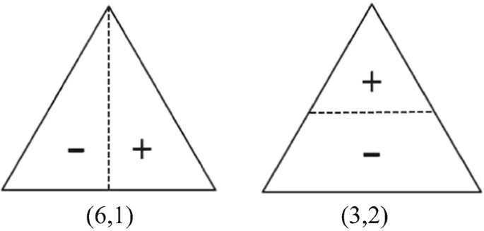

  

  Two sample mode shapes for the equilateral triangular membrane

  Table 6.4 Approximate normal mode frequencies of the equilateral triangular membrane, in order of increasing frequency, approximated by imposing adiabatic invariance and treating the triangle as a 60 ° wedge of a circular membrane of area equal to the hexagon in Fig. 6.12. To maintain the triangular boundary condition, only m = 3i modes can be used where i = 1, 2, 3, …

  Table 6.5 Effective piston area for the four lowest-frequency purely radial normal modes of a circular membrane based on Eq. (6.43)

  Table 6.6 Quantized values of γ_m,n a that determine the normal mode frequencies of a thin disk, t ≪ a, that is clamped at its outer radius, r = a. For larger values of n, γ_m,n a ≅ π[(m/2) + n]

• 9. Modes of a latex diaphragm. A rigidly clamped 20.0-cm-diameter latex sheet is 0.010″ = 254 micron thick. When vibrating in its fundamental mode, f_0,1 = 50.0 Hz.

  • (a) Mass. If the density of latex is ρ = 960 kg/m³, what is the mass of the membrane?

  • (b) Tension. What is the membrane’s tension per unit length?

  • (c) Unperturbed modal frequencies. What are the frequencies and mode numbers of the next five normal modes?

  • (d) Small mass perturbation. If a small piece of putty with mass, M = 0.20 gm, is stuck to the center of the membrane, by how much is each of the frequencies of the fundamental and the next five modes changed? Report your results for parts (c) and (d) in a table with the mode numbers, unperturbed frequencies, and perturbed frequencies.

  • (e) Large lumped-mass loading. If the putty of part (d) above is removed and two magnetic disks, each with a mass of 10.0 gm and a diameter of 4.0 cm, are attached to the top and bottom of the membrane, what will be the frequency of the lowest-frequency normal mode?

• 10. Pressure-driven rectangular membrane. Calculate the area-averaged displacement of a rectangular membrane driven by a time-harmonic excess pressure acoustic, $\delta p(t)=\mathit{\Re e}\left[\hat{\mathbf{p}}{e}^{j\omega\;t}\right]$, in a fluid that is applied to one surface of the membrane, assuming that c_fluid ≫ c = (ℑ/ρ_S)^½ and ω ≪ 2πf_1,1.

• 11. Kettledrum. The circular membrane of a tympani has a diameter of 50.0 cm and a total mass of 31.4 gm and is stretched to a tension per unit length of ℑ = 10,000 N/m.

  • (a) Transverse wave speed. What is the speed of transverse waves on the membrane, ignoring the gaseous restoring force?

  • (b) Fundamental frequency. Determine the fundamental frequency, f_0,1, for the membrane if the volume of the kettle were infinite (i.e., calculate the frequency assuming there is no gas stiffness).

  • (c) Kettle volume. If the kettle volume, V_o, raises the frequency by a factor of 1.27, what is the volume of the kettle? How does this volume compare to the volume of a hemisphere with a diameter that is the same as the membrane?

• 12. Condenser microphone lumped-element model. Using the low-frequency parabolic approximation for the deflection of the microphone’s membrane, subject to a uniform pressure difference, given in Eq. (6.58), the transverse deflection can be expressed in terms of the maximum deflection, z_max = z(0) = a²(δp)/4ℑ.

  $$ z(r)=z(0)\left(1-\frac{r^2}{a^2}\right)\kern1em \mathrm{for}\kern1em 0\le r\le a $$

  (6.98)

  • (a) Effective area. Calculate the effective piston area, A_eff, of the membrane, and express your result as a fraction of the membrane’s area, πa².

  • (b) Effective mass. Determine the effective moving mass, m_eff, of the membrane by calculating the membrane’s kinetic energy. Compare the effective mass to the membrane’s physical mass.

  • (c) Effective stiffness. The potential energy, PE, stored in the microphone’s membrane can be calculated by integrating the work done by the force produced by the excess pressure times the membrane’s displacement over the membrane’s area, dW = (δp 2πr dr) dz. Show that Κ_eff = 2π ℑ by setting PE = ½[Κ_eff z(0)²].

  • (d) Fundamental mode frequency. Using the effective mass and the effective stiffness, calculate the lumped-element approximation to the frequency of the lowest-frequency normal mode, ${\omega}_{0,1}=\sqrt{{\mathrm{K}}_{eff}/{m}_{eff}}$, and then compare your result to the exact result using the Bessel function result of Eq. (6.33).

  • (e) Damping. Determine the mechanical resistance, R_m, necessary to make the membrane’s quality factor Q = 2 using the lumped-element model.

  • (f) Resonance response. What is the response relative to the low-frequency value for the microphone at f_1,0 with Q = 2?

  • (g) Bandwidth. Determine the frequency below f_1,0 at which the microphone’s response exceeds the low-frequency value by 1.0 dB. Report your answer in terms of f_1,0.

  • (h) High-frequency extended response. Determine the frequency relative to f_1,0 at which the microphone’s response is −1.0 dB relative to the low-frequency value above f_1,0. Report your answer in terms of f_1,0.

• 13. Condenser microphone with a stretched stainless-steel diaphragm. The 0.2% yield strength of stainless-steel alloy 316 at room temperatures is 290 MPa, and its mass density is ρ = 7990 kg/m³. A condenser microphone diaphragm made from that alloy has a diameter of 3.0 cm and is 0.001″ (25 microns) thick.

  • (a) Maximum tension/length. Calculate the tension per unit length that would stretch the stainless to its 0.2% yield limit.

  • (b) Transverse wave speed. Calculate the transverse wave speed of the diaphragm when stretched to its 0.2% limit.

  • (c) Fundamental frequency. Calculate the fundamental normal mode frequency f_0,1 for that diaphragm.

  • (d) Open-circuit sensitivity. If a backplate of optimum radius is placed 25 microns from the diaphragm and is polarized by V_bias = 200 V_dc, what will be the low-frequency (i.e., ka < 1) sensitivity of this microphone? Report your result in both V/Pa and in dB re: 1 V/Pa.

• 14. Altec-Lansing Model 21C microphone. This condenser microphone used a ½″ diameter, 50 μm thick glass plate (fused silica, SiO₂) as the diaphragm, instead of a stretched membrane. The glass plate has a sputtered gold coating to make it electrically conductive. If the Young’s modulus of glass is 73.1 GPa and its shear modulus is 31.2 GPa, what is the lowest resonance frequency of the plate if it is clamped at its boundary?

• 15. MEMS microphone. Knowles Acoustics marketed the first commercial microelectromechanical systems (MEMS) silicon diaphragm miniature surface-mount SiSonic^® microphone, shown schematically in Fig. 6.23, in 2003 [29].

  The diaphragm is t = 1.0 μm thick, has an effective diameter of 500 μm, and is made of polycrystalline silicon (polysilicon) with E = 169 GPa and ν = 0.22 [30].

  • (a) Fundamental mode frequency. Calculate the frequency, f_0,1, of the lowest purely radial normal mode, assuming that the boundary is clamped.

  • (b) Diaphragm thickness. Based on the density of polysilicon, ρ_Si = 2.33 gm/cm³, and the atomic mass of silicon, M_Si = 28.08 a.m.u., express t in terms of the number of atoms.

Fig. 6.23

Schematic cross-sectional diagram of a MEMS microphone [30]

References

E. Jahnke, F. Emde, Tables of Functions with Formulae and Curves, 4th edn. (Dover, New York, 1945)
M. Abramowitz, I.A. Stegun, Handbook of Mathematical Functions with Formulas, Graphs and Mathematical Tables, Nat’l. Bur. Standards – Applied Mathematics Series #55 (U.S. Department of Commerce, National Bureau of Standards, Washington, DC, 1964)
M. Greenspan, Simple derivation of the Boltzmann-Ehrenfest adiabatic principle. J. Acoust. Soc. Am. 27(1), 34–35 (1955)
E.C. Wente, A condenser transmitter as a uniformly sensitive instrument for the absolute measurement of sound intensity. Phys. Rev. 10, 39–63 (1917)
H.L.F. Helmholtz, On the Sensation of Tone as a Physiological Basis for the Theory of Music (Longmans & Co, London, 1885). See Ch. III – Analysis of musical tones by sympathetic resonance. Reprinted Dover, 1954; ISBN 0-486-60753-4
J. Tyndall, Sound, 7th edn. (Longmans, Green, and Co, London, 1898), pp. 236–282, see Lecture VI – Singing Flames
J. Zuckerwar, Theoretical response of condenser microphones. J. Acoust. Soc. Am. 64(5), 1278–1285 (1978)
J. Zuckerwar, Principles of operation of condenser microphones, in AIP Handbook of Condenser Microphones, ed. by G. S. K. Wong, T. F. W. Embleton, (American Institute of Physics, New York, 1995). See Chapter 3: ISBN 1-56396-284-5
H.W. Baerwald, The absolute noise level of microphones. J. Acoust. Soc. Am. 12(1), 131–139 (1940)
J.D. Combine, Gaseous Conductors: Theory and Engineering Application (McGraw-Hill, New York, 1941), reprinted (Dover, 1958)
F. Paschen, Ueber die zum Funkenübergang in Luft, Wasserstoff und Kohlensäure bei verschiedenen Drucken erforderliche Potentialdifferenz (On the potential difference required for spark initiation in air, hydrogen, and carbon dioxide at different pressures). Ann. Phys. 273(5), 69–75 (1889)
T.W. Dakin, D. Berg, Theory of gas breakdown, in Progress in Dielectrics, ed. by J. B. Berks, J. Hart, vol. 4, (Wiley, New York, 1962), pp. 152–198
R.S. Dhariwal, J.-M. Torres, M.P.Y. Desmulliez, Electric field breakdown at micrometre separations in air and nitrogen at atmospheric pressure. IEE Proc. Sci. Meas. Technol. 147(5), 261–265 (2000)
M.S. Hawley, F.F. Romanow, J.E. Warren, The Western electric 640AA capacitance microphone: Its history and theory of operation, in AIP Handbook of Condenser Microphones, ed. by G. S. K. Wong, T. F. W. Embleton, (American Institute of Physics, New York, 1995). See Chapter 2; ISBN 1-56396-284-5
G.M. Sessler, J.E. West, D.A. Berkley, G. Morgenstern, Determination of spatial distribution of charges in thin dielectrics. Phys. Rev. Lett. 38(7), 368–371 (1977)
G.M. Sessler, J.E. West, Production of high quasi permanent charge densities on polymer foils by application of breakdown fields. J. Appl. Phys. 43(3), 922–926 (1972)
G.M. Sessler, J.E. West, Electret transducers: A review. J. Acoust. Soc. Am. 53(6), 1589–1600 (1973)
P.W. Chudleigh, Mechanism of charge transfer to a polymer surface by conducting liquid contact. J. Appl. Phys. 47(10), 4475–4483 (1976)
G.M. Sessler, Physical principles of electrets, in Electrets, ed. by G. M. Sessler, (Springer, New York, 1987).; See §2.2.4 (Charging with liquid contact). ISBN 978-3-540-17335-9
P. Horowitz, W. Hill, The Art of Electronics, 2nd edn. (Cambridge University Press, New York, 1989). See Chapter 3
G.W. Elko, K.P. Harney, A history of consumer microphones: The electret condenser microphone meets the micro-electro-mechanical systems. Acoust. Today 5(2), 4–13 (2009)
S.L. Garrett, S. Adams, S. Putterman, I. Rudnick, Resonant nonlinear mode conversion in He II. Phys. Rev. Lett. 41(6), 413–416 (1978)
H. Palevsky, R.K. Swank, R. Grenchik, Design of dynamic condenser electrometers. Rev. Sci. Instrum. 18(5), 298–314 (1947)
G. Rietveld, H.E. van den Brom, Vibration reed electrometer for accurate measurement of electrical currents below 10 pA. IEEE Trans. Instrum. Meas. 56(2), 559–563 (2007)
E. Polturak, S.L. Garrett, S.G. Lipson, Precision acoustic gas analyzer for binary gas mixtures. Rev. Sci. Instrum 57(11), 2837–2841 (1986)
L.D. Landau, E.M. Lifshitz, Elasticity (Pergamon, 1970). See §12; ISBN 0 08 006465 5
T.B. Gabrielson, Frequency constants for transverse vibration of annular disks. J. Acoust. Soc. Am. 105(6), 3311–3317 (1999)
W. Leissa, Vibration of Plates, NASA Report SP-160 (U.S. Government Printing Office, Washington, DC, 1969). reprinted by the Acoustical Society of America, 1993; ISBN 1-56396-294-2
P. Loeppert and S. B. Lee SiSonic™ – The first commercialized MEMS microphone. Solid-State Sensors, Actuators, and Microsystems Workshop, Hilton Head, June 4–8, 2006
W.N. Sharpe Jr., B. Yuan, R. Vaidyanathan, R.L. Edwards, Measurement of Young’s modulus, Poisson’s ratio, and tensile strength of polysilicon, in Proceedings of the 10th International Workshop on Microelectromechanical Systems, (Nagoya, Japan, 1997), pp. 424–429
R.P. Feynman, R.B. Leighton, M. Sands, Introduction, in The Feynman Lectures on Physics, vol. I, (Addison-Wesley, Reading, 1963)
Author information
Authors and Affiliations
Rights and permissions
Open Access This chapter is licensed under the terms of the Creative Commons Attribution 4.0 International License (http://creativecommons.org/licenses/by/4.0/), which permits use, sharing, adaptation, distribution and reproduction in any medium or format, as long as you give appropriate credit to the original author(s) and the source, provide a link to the Creative Commons license and indicate if changes were made.
The images or other third party material in this chapter are included in the chapter's Creative Commons license, unless indicated otherwise in a credit line to the material. If material is not included in the chapter's Creative Commons license and your intended use is not permitted by statutory regulation or exceeds the permitted use, you will need to obtain permission directly from the copyright holder.
Copyright information
© 2020 The Author(s)
About this chapter
Cite this chapter
Garrett, S.L. (2020). Membranes, Plates, and Microphones. In: Understanding Acoustics. Graduate Texts in Physics. Springer, Cham. https://doi.org/10.1007/978-3-030-44787-8_6
Download citation
DOI: https://doi.org/10.1007/978-3-030-44787-8_6
Published:
Publisher Name: Springer, Cham
Print ISBN: 978-3-030-44786-1
Online ISBN: 978-3-030-44787-8
eBook Packages: Physics and AstronomyPhysics and Astronomy (R0)