Elasticity of Solids

Garrett, Steven L.

doi:10.1007/978-3-030-44787-8_4

Steven L. Garrett¹³

Part of the book series: Graduate Texts in Physics ((GTP))

19k Accesses
3 Citations

Abstract

If a solid is initially at rest and equal and opposing forces are applied to that object, Newton’s Second Law guarantees that the object will remain at rest because the net force on the sample is zero. If that object is an elastic solid, then those forces will cause the solid to deform by an amount that is directly proportional to those applied forces. When the forces are removed, the sample will return to its original shape and size. That reversibility is the characteristic that is required if we say the behavior of the solid is “elastic.” This chapter will quantify the elastic behavior of solids by introducing the concepts of stress and strain and expressing their linear relationship through the definition of elastic moduli that depend only upon the material and the nature of the deformation and not upon the shape of the object. Those concepts allow us to generalize Hooke’s law. As before, the combination of a linear equation of state with Newton’s Second Law will now describe wave motion in solids. The introduction of a relaxation time, through the Maxwell model, will let these results be generalized to viscoelastic materials and then be applied to rubber vibration isolators.

You have full access to this open access chapter, Download chapter PDF

Keywords

If we take a piece of solid matter that is initially at rest and apply equal and opposing forces to the sample, Newton’s Second Law of Motion guarantees that the sample will remain at rest because the net force on the sample is zero. If the sample is an elastic solid, then those forces will cause the solid to deform by an amount that is directly proportional to the applied forces. When the forces are removed, the sample will return to its original shape and size. These are the characteristics that are required if we say the behavior of the solid is “elastic.”

Most solids will behave elastically if the forces and their resulting deformations are sufficiently small. If the forces are larger, it is possible to fracture the solid or to cause it to yield so that it does not return to its original shape after the forces are removed. Most metals will fracture if the forces that are applied to them cause deformations that change the length relative to the original length by a few percent. Glass will fracture at less than 1% change in relative length, and rubber can behave elastically for relative deformations that exceed 100%. Different solid materials exhibit a very wide range of behaviors, but most exhibit elastic behavior over some range of deformations.

This chapter will quantify the elastic behavior of solids by introducing the concepts of stress and strain and expressing their linear relationship through the definition of elastic moduli that depend only upon the material and not the shape of the sample. Those concepts will allow us to generalize Hooke’s law. As before, the combination of a linear equation of state, like Hooke’s law, with Newton’s Second Law of Motion, will allow us to describe the wave motion in solids in the next chapter. Further insight will be gained by analyzing vibrational modes of bars, both through the understanding of those modes and by the measurement of those modal frequencies to accurately determine the elastic moduli of the materials.

1 Hooke, Young, Poisson, and Fourier

We begin our investigation into the elasticity of solids by considering the rectangular block of material shown in Fig. 4.1. Since the material is elastic, the force is proportional to the extension, F ∝ Δl; this is the relationship we have called Hooke’s law in previous chapters. If two such pieces are joined end to end to create a piece twice as long, but with the same cross-sectional area, S = wh, then the same force would create twice the extension, 2Δl. We have analyzed this behavior before with springs joined in series, as shown in Fig. 2.3 (right), and also observed twice the extension for the same force. We can therefore write the proportionality of Hooke’s law to exploit this dimensionless measure of deformation as F ∝ (Δl/l). That dimensionless ratio is the strain and it is commonly represented by ε.

Following our analysis of springs in Chap. 2, we can also combine the two solid blocks in parallel so that the overall length of the combination is still l but the cross-sectional area is doubled. To create the same stretch, Δl, the force would have to be doubled. We can combine the dependence on length, l, and on cross-sectional area, S, into a single expression, which is a generalization of Hooke’s law, that introduces a new constant, E, called Young’s modulus. Young’s modulus depends only on the material used to make the block (and its temperature). We will ignore the small difference between the adiabatic and isothermal moduli [1].^{Footnote 1} The ratio of the force, F, to the area, S, over which it is applied, σ = F/S, is called the stress and has the units of pressure [Pa].

$$ \sigma =\frac{F}{S}=E\frac{\Delta l}{l}= E\varepsilon $$

(4.1)

We read Eq. (4.1) as “stress is proportional to strain.” In this case, the constant of proportionality is Young’s modulus, E. Our introduction of this dimensional constant, which is a property of the material, preserves dimensional homogeneity in a way that would please Mr. Fourier (see Sect. 1.6). Since strain, ε, is dimensionless, the units of Young’s modulus are also pressure [Pa].

In Fig. 4.1, we see that in addition to the elongation of l, the height, h, of the rectangle is simultaneously reduced, as is the width, w (not shown). We can introduce another constant to relate the lateral contraction to the longitudinal extension.

$$ \frac{\Delta h}{h}=\frac{\Delta w}{w}=-\nu \frac{\Delta l}{l} $$

(4.2)

That constant of proportionality, ν, is called Poisson’s ratio^{Footnote 2} and is clearly dimensionless.

If the volume of the sample is conserved, when it is strained along its length, as shown in Fig. 4.1, then logarithmic differentiation (see Sect. 1.1.3) can be used to determine the volume-conserving value of Poisson’s ratio.

$$ \frac{\Delta V}{V}=\frac{\Delta l}{l}+\frac{\Delta h}{h}+\frac{\Delta w}{w}=\left(1-2\nu \right)\frac{\Delta l}{l}=0\Rightarrow \nu =\frac{1}{2}\kern1em \mathrm{if}\kern1em \Delta V=0 $$

(4.3)

The deformation of rubber is nearly volume conserving (see Sect. 4.5.1), so its value of Poisson’s ratio is very close to ½, but for most common solid construction materials, like metals and plastics, $ \raisebox{1ex}{$1$}\!\left/ \!\raisebox{-1ex}{$3$}\right. $ ≳ν ≳ ¼. Poisson’s ratio for cork is nearly zero. This makes it a convenient material for sealing wine bottles since it does not expand as force is being applied to push the cork into the neck of a bottle. As we continue our investigation of elasticity, we will determine the fundamental limits on the values of Poisson’s ratio that are imposed by material stability and energy conservation.

2 Isotropic Elasticity

If the elastic material is homogeneous and isotropic, its elastic behavior is completely specified by E and ν. Our introduction of E and ν was convenient, since our sample had a rectangular shape and was unconstrained along the sides and the forces were normal to the ends where they were applied. The choice of E and ν is not our only option for the two independent constants required to specify the elastic behavior of an isotropic solid. As we are about to demonstrate by the use of the principle of superposition (see Sect. 1.4), we can relate E and ν to other moduli that are convenient for the specification of an isotropic material’s response to different combinations of stresses.

2.1 Bulk Modulus

We can use Young’s modulus, E, and Poisson’s ratio, ν , to calculate the deformation of a solid that is subject to a hydrostatic compression. If we imagine our solid being submerged in a fluid, as the fluid pressure increases, the volume of the solid will decrease, but its shape will remain the same. Pascal’s law guarantees that the hydrostatic pressure will be the same on all faces if the sample is at rest and the size of the sample is small enough that any gradients in the gravitational field can be ignored. This situation is shown schematically in Fig. 4.2. We can combine Pascal’s law with the principle of superposition to calculate the change in length of any side and combine those changes using Eq. (4.3) to compute the relative change in volume of the sample, ΔV/V.

We start by calculating the change in length, Δl_l, due to the force, F_l, on the ends normal to the l-direction. The pressure, P, provides the stress, σ = P.

$$ \frac{\Delta {l}_l}{l}=-\frac{\sigma }{E} $$

(4.4)

The minus sign reminds us that the increased pressure decreases the length of the sample. At the same time, the pressure, P, should produce the same strain in the height, (Δh_h/h) = − (σ/E). Poisson’s ratio determines the influence this change in height will have on the change in length.

$$ \frac{\Delta {l}_h}{l}=-\nu \frac{\Delta {h}_h}{h}=\nu \frac{\sigma }{E} $$

(4.5)

Since both the pressure and the material are isotropic, there is an equal change in length, Δl_w/l, caused by Δw/w and Poisson’s ratio, ν. The total strain in length, Δl/l, must be the sum (i.e., superposition) of these three contributions.

$$ \frac{\Delta l}{l}=\frac{\Delta {l}_l}{l}+\frac{\Delta {l}_h}{l}+\frac{\Delta {l}_w}{l}=-\frac{\sigma }{E}\left(1-2\nu \right) $$

(4.6)

This result now allows us to relate the volumetric strain, ΔV/V, to the hydrostatic pressure, P = σ, again using logarithmic differentiation, as in Eq. (4.3), and recognizing that the strain along all three of the sample’s axes must be the same.

$$ \frac{\Delta V}{V}=\frac{\Delta l}{l}+\frac{\Delta h}{h}+\frac{\Delta w}{w}=-3\left(1-2\nu \right)\frac{\sigma }{E} $$

(4.7)

We can now define a third elastic modulus, known as the bulk modulus, B, to relate changes in hydrostatic pressure to volumetric strain.

$$ P=\sigma =-B\frac{\Delta V}{V}=-\frac{E}{3\left(1-2\nu \right)}\frac{\Delta V}{V} $$

(4.8)

In addition to providing the relationship between the bulk modulus, Young’s modulus, and Poisson’s ratio, Eq. (4.8) restricts Poisson’s ratio to being less than one-half. To guarantee the stability of matter, the bulk modulus can never be negative. If the bulk modulus were negative, then the application of a small amount of pressure would cause the volume of the material to increase rather than decrease. The product of that change in pressure and the change in volume would do work on the surroundings. This would allow us to get useful work out of any material with B < 0 and would violate energy conservation. Similarly, if the solid were immersed in a fixed volume of liquid and the pressure of the liquid decreased (due to a change in temperature?), then the solid would become smaller, decreasing the fluid pressure further, and ultimately the solid would disappear [2].

2.2 Modulus of Unilateral Compression

The same use of superposition that allowed us to relate the bulk modulus, Young’s modulus, and Poisson’s ratio can be exploited again to calculate the modulus of unilateral compression, sometimes also known as the dilatational modulus. We will use D to designate this modulus. The modulus of unilateral compression is similar to Young’s modulus except that the cross-section is not allowed to change, that is, Δh_l/h = Δw_l/w = 0, when Δl_l/l ≠ 0. An example of a deformation due to a unilateral compression is shown in Fig. 4.3. This combination of pressure and strain is important for the propagation of plane longitudinal waves in solids.^{Footnote 3}

We would expect the modulus of unilateral compression to be greater than Young’s modulus, since it should be more difficult to compress a sample if the walls are not permitted to bulge out. As before, we will superimpose three contributions to the strain in the length.

$$ \frac{\Delta {l}_l}{l}=\frac{1}{E}\frac{F_l}{S_l}-\frac{\nu }{E}\frac{F_h}{S_h}-\frac{\nu }{E}\frac{F_w}{S_w}=\frac{1}{E}\left[\frac{F_l}{S_l}-\nu \left(\frac{F_h}{S_h}+\frac{F_w}{S_w}\right)\right] $$

(4.9)

$$ \frac{\Delta {l}_h}{h}=\frac{1}{E}\left[\frac{F_h}{S_h}-\nu \left(\frac{F_l}{S_l}+\frac{F_w}{S_w}\right)\right] $$

(4.10)

$$ \frac{\Delta {l}_w}{w}=\frac{1}{E}\left[\frac{F_w}{S_w}-\nu \left(\frac{F_l}{S_l}+\frac{F_h}{S_h}\right)\right] $$

(4.11)

Imposition of the constraint that Δh/h = Δw/w = 0 dictates the required stress needed to keep the cross-section constant. Those stresses can be determined by simultaneous solution of Eqs. (4.10) and (4.11).

$$ \frac{F_h}{S_h}=\frac{F_w}{S_w}=\frac{\nu }{1-\nu}\frac{F_l}{S_l}=\left(\frac{\nu }{1-\nu}\right)\sigma $$

(4.12)

Substitution of this result back into Eq. (4.9) relates the strain in l to the stress in the direction normal to l.

$$ \frac{\Delta {l}_l}{l}=\frac{1}{E}\left(1-\frac{2{\nu}^2}{1-\nu}\right)\frac{F_l}{S_l}=\left(\frac{\left(1+\nu \right)\left(1-2\nu \right)}{1-\nu}\right)\frac{\sigma }{E} $$

(4.13)

By inverting this expression, we can write the modulus of unilateral compression, D, in terms of Young’s modulus and Poisson’s ratio.

$$ \sigma =D\frac{\Delta l}{l}=\frac{\left(1-\nu \right)}{\left(1+\nu \right)\left(1-2\nu \right)}E\frac{\Delta l}{l} $$

(4.14)

Figure 4.4 shows that D/E > 1, if ν > 0, as expected, since the sample is “stiffened” if the cross-section is constrained to remain unchanged.

The appearance of (1 + ν) in the denominator of Eq. (4.14) implies that if Poisson’s ratio is negative, it cannot be more negative than −1 without violating the stability requirement, so −1 < ν ≤ ½.

2.3 Shear Modulus

A hydrostatic compression changes the volume of a sample but not its shape. A shear deformation, shown in Fig. 4.5, changes the shape of a sample but not its volume. Figure 4.5 shows one face of an initially cubical sample, l = h, which is rigidly supported along its left face and has a shearing force, F = Mg, applied along the opposite face by a suspended mass, M. The resulting shear strain will deform the square into a rhombus. Since h has not changed, the areas of the square and rhombus are equal, as are the volumes of their corresponding solids, the cube and rectangular parallelepiped (sometimes referred to as a rhomboid).

We can again use superposition to express the shear modulus in terms of Young’s modulus and Poisson’s ratio. This process is simplified if we examine Fig. 4.5 and realize that the shear deformation has taken the two diagonals of the square, which were originally of equal length, and made one diagonal shorter and the other longer, D_long > D_short. The cube is represented in Fig. 4.5 by a two-dimensional cross-section that ignores the width, w, since it is not changed by the shearing. The compression and expansion of the two diagonals can be reproduced if the original square is circumscribed by a larger square that is rotated by 45 ° with respect to the original. The larger square has edge lengths, $ {l}^{\prime }={h}^{\prime }=l\sqrt{2} $.

If we apply compressive forces, $ {F}^{\prime }=F\sqrt{2} $, to parallel faces, then the applied stress would be unchanged, since the surface area of the larger cube is $ \sqrt{2} $ greater than that of the original cube. Those compressive forces will make one of the diagonals shorter. Similarly, if an equal tensile stress is applied to the cube’s orthogonal faces, then the other diagonal is lengthened. The net forces and the net torque are zero, so the cube remains at rest during deformation. Also, we see that a pure shear is equivalent to the superposition of equal compressive and tensile stresses applied at right angles to each other and at 45 ° to the original faces of the cube.

We again superimpose the two orthogonal stresses to calculate the change in the length and the height of the deformed cube.

$$ \frac{\Delta {l}^{\prime }}{l^{\prime }}=\frac{\Delta {D}_{long}}{D}=-\frac{\Delta {h}^{\prime }}{h^{\prime }}=-\frac{\Delta {D}_{short}}{D}=\frac{1}{E}\frac{F}{S}+\nu \frac{1}{E}\frac{F}{S}=\left(\frac{1+\nu }{E}\right)\frac{F}{S} $$

(4.15)

In Fig. 4.5, the strain is a dimensionless quantity, as is the angle, θ , by which the cube is sheared. (Keep in mind that in these calculations, D is the unstrained diagonal, not the modulus of unilateral compression.)

$$ \tan \theta \cong \theta =\frac{\Delta y}{l}=\sqrt{2}\frac{\Delta D}{l}=2\frac{\Delta D}{D}=2\left(\frac{1+\nu }{E}\right) $$

(4.16)

The far-right term takes advantage of the fact that we are assuming linear elastic behavior, so Δy < < l. Inverting this result leads to the definition of the shear modulus, G, that again allows us to assert Hooke’s law as “stress is proportional to strain,” this time for shearing stresses.

$$ {\sigma}_{yx}=\frac{F_y}{S_x}= G\theta =\frac{E}{2\left(1+\nu \right)}\theta $$

(4.17)

In this version of Hooke’s law, a new nomenclature has been introduced that is convenient for the description of stress. σ_yx represents a force, F_y, that is applied in the y direction on a surface of area, S_x, which has its normal in the x direction. In this notation, the normal hydrostatic stresses would be σ_xx = σ_yy = σ_zz = P and σ_xy = σ_yz = σ_zx = 0, since fluids cannot sustain static shearing forces.^{Footnote 4}

Again, for stability, we must insist that G > 0, so ν > −1. Combined with the similar restriction imposed by the bulk modulus, the values of Poisson’s ratio are therefore restricted: −1 < ν < ½. Most materials have Poisson’s ratios that are between zero (e.g., cork) and ½ (e.g., rubber). Auxetic materials, which have negative values of Poisson’s ratio, are uncommon. Love reported ν = −0.14 for single-crystal pyrite [3]. Most auxetic materials are anisotropic, have very low mass densities, and usually involve some complicated internal structure, like solid foams. A Poisson’s ratio as small as ν = −0.7 has been reported for solid foam with a tetrakaidecahedral (14-sided) unit cell [4].

2.4 Two Moduli Provide a Complete (Isotropic) Description

If a solid is isotropic and homogeneous, then two moduli provide a complete description of the solid’s elastic behavior. The results of the calculations that relate Young’s modulus, Poisson’s ratio, the bulk modulus, the modulus of unilateral compression (or dilatational modulus), and the shear modulus are summarized in Table 4.1.^{Footnote 5}

Table 4.1 For any isotropic solid, two elastic constants are sufficient to completely specify the solid’s elastic behavior. Given any two known elastic moduli, listed in the left-hand column, equations are provided for the calculation of the other three isotropic elastic moduli

Full size table

3 Real Springs

In Chap. 2, we defined a spring constant that provided a parameter, Κ, to relate forces and displacements governed by Hooke’s law. That definition allowed us to explore the behavior of simple harmonic oscillators consisting of masses, springs, and dashpots. Having developed a system for understanding the elastic behavior of solids, we can now explore a small amount of the vast territory that is dedicated to the design of a highly engineered product that has a very significant impact on the design or isolation of vibrating systems – the spring.

Real springs are much more complicated than Hooke’s law may lead one to believe. Our analysis of the simple harmonic oscillator, in Chap. 2, represented the spring through a single parameter, the spring stiffness, Κ, which concealed the multiple design trade-offs that must be made to approach optimum performance for any spring. In addition to stiffness, attention must also be paid to the spring’s moving mass; to limitations on the tensile stresses that might cause the material to yield or fracture, thus exceeding the elastic limit (see Fig. 1.4); or to application of compressive stresses that would cause buckling (see Sect. 4.3.4), as well as issues related to fatigue life in a material that is subjected to fully reversing cyclic loading for millions or billions of cycles [5].

In this section, we will explore only a few strategies for shaping materials in ways that make them suitable for applications where they are intended to store (and in some cases, absorb) elastic energy using the spring materials efficiently. We will start with simple use of the bulk material to provide stiffness, but then look at how shapes such as cantilevered beams, tubes in torsion, and helical coils produce acceptable and convenient trade-offs in a few applications and how rubberlike materials are used as springs for vibration isolation where they simultaneously provide both elasticity and damping.

3.1 Solids as Springs

Although the majority of spring applications require forming and shaping of the elastic material, as well as surface treatments (e.g., shot peening, tumble deburring) and heat treatments (e.g., precipitation hardening, quick quenching) [6], there are a few circumstances where the material is used “in bulk,” as a block, rod, or tube to provide compressional or shear stiffness. This is most common with rubber springs used as vibration isolators. We will postpone discussion of rubber springs until later in this chapter because the viscoelastic behavior of those elastomeric materials can simultaneously contribute damping as well as stiffness. Here we will examine two piezoelectric accelerometer designs and a resonant piezoelectric underwater sound source that use the elasticity of the bulk materials to provide stiffness.^{Footnote 6}

An accelerometer is a vibration measurement sensor that converts mechanical accelerations into an electrical signal that can be displayed and/or recorded by some electronic measurement instrument. The base of an accelerometer is usually attached to some vibrating structure using a threaded stud, a magnet, an adhesive or wax, etc., that attempts to ensure that the motions of the sensor and of the vibrating structure are identical. As we have seen from our study of the displacement-driven simple harmonic oscillators in Sect. 2.5.6, if the driving frequency, ω, is less than the natural frequency, $ \omega <{\omega}_o=\sqrt{\mathrm{K}/m} $, then the displacement of the spring is directly proportional to the force produced by the acceleration, a, of the mass, m: xe^jω t = −mae^jω t/Κ.

Figure 4.6 shows cross-sectional diagrams of two types of piezoelectric accelerometers. We start by calculating the stiffness of the version (Fig. 4.6, right) that compresses a test mass (sometimes also called a seismic mass or a proof mass) against a hollow cylinder made of a ferroelectric ceramic material^{Footnote 7} using a steel “preload stud.” Since ceramic materials are much stronger in compression than under tension, static compression provided by the preload stud guarantees that the piezoelectric spring never goes into tension, as well as holding the mass-spring “sandwich” together. The total stiffness of the cylinder and stud will be the sum of their stiffnesses: Κ_total = Κ_stud + Κ_piezo.

If we treat the pre-load stud as a thin rod, then its stiffness, Κ_stud, will be related to its geometry and Young’s modulus of the material that is used to make the stud. We will let the length of the stud (between the mass and the base) be l, let its diameter be D_stud, and assume the stud is made of some generic steel. The stiffness of the piezoelectric tube will depend upon its Young’s modulus and its inner and outer radii, a_in and a_out. Its elastically active length, l, is the same as the stud’s length. Using the appropriate cross-sectional areas, the stiffnesses are given by

$$ {\mathrm{K}}_{stud}=\frac{E_{steel}\left(\frac{\pi }{4}{D}_{stud}^2\right)}{l}\kern1em \mathrm{and}\kern1em {\mathrm{K}}_{piezo}=\frac{\pi {E}_{piezo}\left({a}_{out}^2-{a}_{in}^2\right)}{l} $$

(4.18)

Let’s assign some nominal values to those one dimensions and to the elastic moduli. For the stud, let D_stud = 2.0 mm (about the correct value for a 4–40 machine screw) and let l = 6.0 mm. Representative values for steel^{Footnote 8} are E_steel = 195 GPa and ρ_steel = 7700 kg/m³. We’ll choose lead zirconium titanate (PZT) as our piezoelectric (ferroelectric) ceramic, with representative values of E_PZT = 50 GPa and ρ_PZT = 7500 kg/m³. The ceramic tube will have the same length as the stud with an outer radius a_out = 4.0 mm and an inner radius a_in = 2.0 mm. To be relatively consistent with the dimensions in Fig. 4.6, the test mass will be a steel cylinder with D_mass = 12.0 mm and a height h = 4.0 mm. Plugging these values into Eq. (4.18) makes Κ_stud = 1.02 × 10⁸ N/m and Κ_piezo = 3.14 × 10⁸ N/m for a total stiffness of Κ_total = 4.16 × 10⁸ N/m.

For the test (seismic) mass, m_test = ρ_steel (π/4) D_mass² h = 3.5 × 10⁻³ kg. Based on Eq. (2.27), we should add one-third of the mass of the springs to the test mass to approximate the dynamic mass, m_o.

$$ {m}_o={m}_{test}+\left(\frac{m_{PZT}+{m}_{stud}}{3}\right)={m}_{test}+\frac{\pi }{12}\left[4{\rho}_{PZT}\left({a}_{out}^2-{a}_{in}^2\right)l+{\rho}_{steel}{D}_{stud}^2l\right] $$

(4.19)

Using the same values for the dimensions and the mass densities, m_o = 4.10 × 10⁻³ kg, so $ {f}_o=\left({\omega}_o/2\pi \right)=\sqrt{{\mathrm{K}}_{total}/{m}_o}/2\pi =50.7\kern0.5em \mathrm{kHz} $.

To demonstrate that these numbers are not unrealistic, Fig. 4.7 shows the calibration card for a typical accelerometer of this type that has been in use in my laboratory for decades. The relative response (in dB) as a function of frequency shows a peak at just below 30 kHz. The response is constant with an increase of 1.0 dB in the sensitivity at 10 kHz but is “flat” (frequency independent) below that frequency where the sensor is operating well within its stiffness-controlled frequency regime, ω < ω_o.

Let’s repeat the analysis for the “shear mode” accelerometer shown in Fig. 4.6 (left and center). It consists of three flat quartz (SiO₂) plates supported along their inside surfaces by a post attached to the accelerometer’s case and along their outside surfaces by three masses that are attached to each other by a retaining ring. As the case moves upward, the masses exert a downward shear force on the quartz plates in much the same way as the suspended mass exerts a static shear force on the sample diagrammed in Fig. 4.5 (left). We will use G_quartz = 2.23 × 10¹⁰ Pa as the shear modulus of quartz and ρ_quartz = 2650 kg/m³. We’ll let m_test = 5 grams for the test mass (0.005 kg) and choose plausible dimensions for the quartz plates: l = 2.0 mm, h = 4.0 mm, and w = 5.0 mm. Using the appropriate cross-sectional areas, the stiffnesses are given by

$$ {\mathrm{K}}_{quartz}=-\frac{F_y}{\Delta y}={G}_{quartz}\frac{wh}{l} $$

(4.20)

Remembering that the stiffnesses, Κ_quartz, of each of the three plates are additive, Κ_total = 3Κ_quartz = 6.7 × 10⁸ N/m. The total mass for the three quartz plates is 3m_quartz = 0.318 gram, one-third of which is added to the test mass to make m_o = 5.11 × 10⁻³ kg. Again, $ {f}_o=\left({\omega}_o/2\pi \right)=\sqrt{{\mathrm{K}}_{total}/{m}_o}/2\pi =57.6\kern0.5em \mathrm{kHz} $.

The piezoelectric effect will produce an alternating electrical output based on the alternating stresses in the piezoelectric elements in either accelerometer design. This is not the time to belabor the differences between the two designs or their electrical transduction mechanisms, since these accelerometers were introduced primarily as vibration sensors and simple examples of the direct use of the elastic properties of solids to provide stiffness in real (i.e., useful) physical systems.

Since the piezoelectric effect is both linear and reversible, it is also possible to drive the piezoelectric elements as “motors.” The next example is a Tonpilz^{Footnote 9} transducer that is common in naval SONAR systems and torpedo guidance systems [7].

Figure 4.8 shows a detailed drawing of such an underwater projector on the top [8] and a simplified cross-sectional diagram on the bottom [9]. We will further simplify our analysis by treating this transducer as two masses joined by a spring. As with the coupled harmonic oscillators in Sect. 2.7, this transducer is a one-dimensional oscillator that has two degrees of freedom corresponding to the positions of the head and tail masses. It will therefore possess two normal mode frequencies: a lower-frequency symmetric mode (both masses moving in-phase) and a higher-frequency antisymmetric mode. In this case, the symmetric mode corresponds to a uniform translation with both masses moving at the same velocity in the direction joining their centers. The frequency of that mode is zero because there is no restoring force. Our interest is in the antisymmetric mode, where the head and tail masses move in opposite directions, thus compressing or expanding the spring that joins them.

The modal frequency for such a combination is well-known (see Sects. 2.7.1, 2.7.2, and 2.7.3) because it is analogous to the vibration of a diatomic molecule [10]. If the spring were massless, then the frequency of the antisymmetric mode is $ {\omega}_a=\sqrt{\mathrm{K}/\mu } $, where μ = (m₁m₂)/(m₁ + m₂) is known as the reduced mass.

This result is easy to visualize for m₁ = m₂. In that case, we know that the amplitude of the motions of both masses must be equal and opposite, so the midpoint of the spring will be a node. The normal mode frequency corresponds to all parts of the system oscillating at the same frequency. We can exploit that fact to calculate ω_a by calculating the motion of one mass and one spring of twice the spring constant that has half the total length: $ {\omega}_a=\sqrt{2\mathrm{K}/{m}_1}=\sqrt{\mathrm{K}/\mu } $. We will use the same approach to calculate the resonance frequency of our Tonpilz transducer that has different values for masses, m₁ ≠ m₂, and a spring, being the piezoelectric stack and tensioning rod, which will also contribute non-negligible mass.

First, let’s choose some reasonable values for the components in our Tonpilz example. Since the objective of this design is the generation of sound in water, we would like the tail mass to be larger than the head mass so that the motion of the end in contact with the water will be greater than the motion of the “counter weight” provided by the tail mass. As will be demonstrated in Sect. 12.8.3, a circular piston whose circumference is less than the wavelength of the radiated sound, 2πa < λ_fluid = c_water/f, has to accelerate a mass of fluid, m_rad, that is equivalent to the mass of fluid contained in a cylindrical volume with the same area as the piston, πa², and a height, h = (8/3π)a. If we let the radius of the head mass be 5.0 cm, then the radiation mass is m_rad = (8/3) a³ρ_water = 0.333 kg.

Since the design goal is to make the head mass as light as possible, the radiation mass places a natural limit on how a natural limit on how advantageous it might be to make the head mass small. For this example, let’s make the head mass (including the radiation mass of the fluid) about twice the radiation mass, m_h = 0.70 kg. The head mass should be as stiff as possible so that it acts as a piston and does not flex. That combination of lightness and stiffness can be improved by making the head mass “ribbed” to increase rigidity and reduce its moving mass. Such a “ribbed piston” is shown in Fig. 4.9. We will let the tail mass be five times the head mass, m_t = 5m_h = 3.5 kg.

The spring’s stiffness will again be provided by a stack of piezoelectric ceramic rings that are pre-compressed by the tensioning rod. Let the diameter of the tension rod be D_rod = 6.0 mm and choose the outer and inner radii of the piezoelectric rings to be a_out = 2.0 cm and a_in = 1.5 cm. The length of the stack will be L = 15.0 cm. Using the previous values of Young’s modulus and mass density for steel and PZT, the stiffnesses and masses are as follows: Κ_rod = 3.67 × 10⁷ N/m, Κ_PZT = 1.83 × 10⁸ N/m and Κ_total = 2.20 × 10⁸ N/m; m_rod = 32.7 gm and m_PZT = 0.618 kg, so m_s = 0.651 kg.

Since the two masses are not equal, we will need to properly apportion the moving mass, m_s, and Κ_total of the PZT stack and steel rod about the vibration node. We will use the equality of the frequencies on either side of the node, as we did in Sect. 3.6.2, to determine the location of the node and yield the antisymmetric normal mode frequency. If we let the node be a distance, b, from the attachment point of the head mass, m_h, then the separation between the attachment point of the tail mass, m_t, and the node must be L – b.

We have used the fact that the stiffness-length product is a constant before (see Sect. 2.2.2), although now we see it also as a direct consequence of our definition of Young’s modulus in Eq. (4.1): ΚL = FL/Δl = ES. That allows us to write the stiffness of the spring between the node and the head mass as Κ_h = (Κ_totalL)/b and the stiffness of the spring between the tail mass and the node as Κ_t = (Κ_totalL)/(L-b). Since m_t = 5m_h, we expect 5(L-b) ≅ b. If we also scale the moving mass of the spring, then the equality of the normal mode frequencies can be solved to provide the value of b.

$$ {\omega}_h^2=\left(\frac{{\mathrm{K}}_{total}L}{b}\right)\frac{1}{m_h+\frac{bm_s}{3L}}=\left(\frac{{\mathrm{K}}_{total}L}{L-b}\right)\frac{1}{m_t+\frac{\left(L-b\right){m}_s}{3L}}={\omega}_t^2 $$

(4.21)

Solving Eq. (4.21) will provide the b/L ratio.

$$ \frac{b}{L}=\frac{m_t+\frac{m_s}{3}}{m_t+{m}_h+\frac{2{m}_s}{3}} $$

(4.22)

For the values used in this example, b/L = 0.802. (This would also tell us where we would want to support this projector so that none of its vibrations are communicated through the support structure.) Plugging b/L back into Eq. (4.21) gives f_h = f_t = 2.82 kHz. If the speed of sound in water is c_water = 1500 m/s, then 2πa = 31.4 cm and λ_fluid = c/f_h = 53.2 cm > 2πa, so the radiation mass assumption was valid. This result is close to what would have been the normal mode frequency, $ {f}_a=\sqrt{{\mathrm{K}}_{total}/\mu }/2\pi =3.1\kern0.5em \mathrm{kHz} $, using the reduced mass μ = (m₁m₂)/(m₁ + m₂) = 0.583 kg and assuming that the spring (the piezoelectric stack and tension rod) was massless.

These three examples of the direct use of solids as springs have been restricted to solid samples with a small aspect ratio, which is l ≲ w ≅ h, for the accelerometers, and to forces on the spring being applied longitudinally by the motor mechanism (i.e., the piezoelectric stack) and inertial effects in the Tonpilz case. It is rare to see long thin rods or bars being used as linear springs because the forces necessary to bend such a sample are smaller than the forces that would produce an equivalent longitudinal compression. This restriction will be quantified in the next sub-section. Also, long thin bars that are subject to compression can spontaneously buckle (i.e., collapse catastrophically) if the force exceeds a threshold value as discussed in Sect. 4.3.4.

3.2 Flexure Springs

Cantilevered beams are used as springs in applications that range from automotive suspensions to micromachined silicon sensors (like the beam from the atomic force microscope shown in Fig. 2.36). If you hold a meter stick with both hands at eye level,^{Footnote 10} with the numbers facing upward or downward, it is possible to apply torques to the two ends, as shown in Fig. 4.10, that will bend the meter stick into a smooth curve that corresponds (approximately) to the arc of a circle. If the numbered surface of the meter stick is facing toward you, then it will be very difficult to bend the meter stick vertically. Given enough torque, it might squirm (rotate into the previous orientation) or possibly fracture, although it does bend easily and reversibly if it is held flat (number side up or down). The radius of curvature, R, as expressed in Eq. (4.33), will be infinite before the meter stick is bent. As the bending increases, the radius will become shorter. In Fig. 4.10, R ≅ 2.5 L, where L is the length of the meter stick.

What is happening to the material when the stick is bent and what is providing the restoring force that returns the stick to its straight condition after the torques are removed? When the stick is curved, as shown in Fig. 4.10, the material near the top of the stick is placed in tension and the material near the bottom of the stick is placed in compression. Since the stresses change sign going from the top of the stick to the bottom, there must be some surface near the middle that is unstressed. That surface is called the neutral plane. Figure 4.11 (left) shows a small segment of the bent beam (meter stick). The dashed line corresponds to the position of that neutral plane.

If there are no additional tensile or compressive forces applied to the beam, just the applied torque, then below the neutral plane, the compressive strain is proportional to the distance, h, below the neutral plane. Above the neutral plane, the tensile strain is also proportional to the distance, h, above the neutral plane.

$$ \frac{\Delta l}{l}=\frac{h}{R} $$

(4.23)

To work out the forces so they can be summed (integrated) to calculate the bending moment (i.e., the restoring torque), we will consider a differential segment of a rectangular beam that is w wide, t thick, and rigidly clamped at x = 0, as shown schematically in Fig. 4.11 (left). When h = +(t/2), the uppermost surface of the element is stretched from its equilibrium length by an amount, Δl = +δx, and the lowermost surface at h = −(t/2) is compressed by Δl = −δx.

By our definition of Young’s modulus in Eq. (4.1), the stress (force per unit area) is also proportional to the distance from the neutral plane. Letting dS = w dh, the force, δF, produced by the filament, dh, thick and w wide, a distance, h, above the neutral plane, is related to the strain by Young’s modulus, E.

$$ \frac{dF}{dS}=E\frac{\delta x}{dx} $$

(4.24)

The strain, δx/dx, can be calculated using Garrett’s First Law of Geometry (as stated in Sect. 1.1).

$$ \frac{\delta x}{dx}=\frac{h\tan \phi }{dx}\cong h\frac{\phi }{dx}\kern1em \Rightarrow \kern1em \frac{dF}{dS}=E\frac{h\phi}{dx} $$

(4.25)

In Fig. 4.11 (left), the forces cancel but their bending moment about the neutral plane, 𝔐, is non-zero. That moment can be calculated by integration of the force times the distance from the neutral plane.

$$ \mathfrak{M}=\int h\; dF=\frac{E\phi}{dx}\int {h}^2\; dS\equiv \frac{E S{\phi \kappa}^2}{dx}\kern1em \mathrm{where}\kern1em {\kappa}^2=\frac{\int {h}^2\; dS}{S} $$

(4.26)

The square of radius of gyration, κ², will depend upon the shape of the beam. κ² is calculated below for the two cases shown in Fig. 4.11 (right).

$$ {\displaystyle \begin{array}{c}{\kappa}_{bar}^2=\frac{w\int_{-t/2}^{t/2}{h}^2\; d y}{wt}=\frac{t^2}{12}\\ {}{\kappa}_{rod}^2=\frac{4\int_0^{\pi /2}\left({a}^2{\sin}^2\;\theta \right)\kern0.5em \left(a{\cos}^2\theta \right)\;a\; d\theta}{\pi {a}^2}=\frac{a^2}{4}\end{array}} $$

(4.27)

The stiffness of a beam in flexure depends not only upon the material but also its distribution with respect to the neutral axis. The effects of this material distribution are quantified by the square of the radius of gyration, κ². That is why steel used in construction frequently has a cross-section that is in the shape of an “I” or “H” to place more material farther from the neutral plane. This strategy will be limited because too much material separated from the neutral plane by too little “webbing” will allow the shape to become distorted, or twisted, when loaded, like trying to bend the meter stick against the tall dimension (the numbers facing you, instead of the edge facing you) in our first bending example.

Due to the critical importance of the moment of inertia^{Footnote 11} and the radius of gyration for structural engineering, there are numerous handbooks that provide the results for these integrations over nearly any imaginable cross-section. My favorite compilation for such results, as well as for the stresses on pressure vessels, bending of beams and plates, vibration of structures, etc., is Roark’s Formulas for Stress and Strain [12]. A portion of one page from Appendix A.1, “Properties of Sections,” taken from that book, is shown in Fig. 4.12.

For small deflections, application of Garrett’s First Law of Geometry suggests that the angle, ϕ, is the same as the negative of the difference in the slope of the neutral plane at x = 0 and at x = dx, which can be estimated using the first two terms in a Taylor series.

$$ \phi =-\left[{\left(\frac{\partial y}{\partial x}\right)}_{x+ dx}-{\left(\frac{\partial y}{\partial x}\right)}_x\right]=-\left(\frac{\partial^2y}{\partial {x}^2}\right) dx $$

(4.28)

In Fig. 4.11 (left), (∂y/∂x)_x = 0 = 0, but Eq. (4.28) would be correct even if that were not the case. Substitution of Eq. (4.28) for ϕ back into Eq. (4.26) provides the relation between the bending moment, 𝔐, and the curvature of the differential element that will be useful for the calculation of the flexural vibration of beams in Sect. 5.3.

$$ \mathfrak{M}=- ES{\kappa}^2\frac{\partial^2y}{\partial {x}^2} $$

(4.29)

The work done to bend the differential element in Fig. 4.11 (left) can be calculated in terms of the angle of the bend, again by use of Garrett’s First Law of Geometry, ϕ = dx/R. The bending moment, 𝔐, in Eq. (4.26) can be expressed in terms of that angle.

$$ \mathfrak{M}=\frac{ES{\kappa}^2}{dx}\phi $$

(4.30)

The amount of work, dW, required to bend that differential element from its equilibrium condition (straight) into an arc of angle, ϕ, will be the integral of the moment.

$$ dW={\int}_0^{\phi}\mathfrak{M}\left({\phi}^{\prime}\right)\;d{\phi}^{\prime }=\frac{1}{2}\frac{ES{\kappa}^2}{dx}{\phi}^2 $$

(4.31)

Substituting the expression for ϕ, derived in Eq. (4.28), into Eq. (4.31) provides an expression for the change in potential energy that is done by the work of bending the differential element that is in a convenient form for integration along bars.

$$ d(PE)=- dW=\frac{ES{\kappa}^2}{2}{\left(\frac{\partial^2y}{\partial {x}^2}\right)}^2 dx $$

(4.32)

Let’s now apply Eq. (4.26) to the cantilevered beam that was drawn by Galileo and shown in Fig. 2.27. That (wooden) beam is built into a wall that constrains the slope of the beam to be zero as it leaves the wall. We can let y (x) be the transverse deflection of the beam from equilibrium as a function of distance, x, from the wall. The vertical component of the force, F_v, which causes the deflection, will be the weight of the mass, M, attached at the beam’s end x = L, with F_v = Mg. Equation (4.33) provides the reciprocal of the radius of curvature of the beam, R⁻¹, at any location, x.

$$ \frac{1}{R}=\frac{\frac{d^2y}{dx^2}}{{\left[1+{\left(\frac{dy}{dx}\right)}^2\right]}^{2/3}}\cong \frac{d^2y}{dx^2}\kern1em \mathrm{if}\kern1em {\left(\frac{dy}{dx}\right)}^2<<1 $$

(4.33)

Since only small deflections are being considered, the approximate expression for the radius of curvature can substituted into Eq. (4.26).

$$ \mathfrak{M}(x)= Mg\left(L-x\right)=-\frac{ES{\kappa}_{beam}^2}{R}=-\frac{E(wt){t}^2}{12}\frac{d^2y}{dx^2} $$

(4.34)

This provides an ordinary differential equation for the deflection, y (x).

$$ \frac{d^2y(x)}{dx^2}=-\frac{12 Mg}{Ewt^3}\left(L-x\right)\cong \frac{1}{R}=\frac{1}{h}\frac{\Delta l}{l} $$

(4.35)

The right-hand side of Eq. (4.35) is just a polynomial; hence, its integration (twice) from the wall at x = 0 to the end at x = L is easy to perform.

$$ y(x)=-\frac{6 Mg}{Ewt^3}\left({Lx}^2-\frac{x^3}{3}\right) $$

(4.36)

The leading minus sign shows that the deflection is downward for the addition of a positive mass. It is worth noticing that this solution satisfies the boundary conditions that the wall imposes on the beam: y (0) = 0 and (dy/dx)_x = 0 = 0. The deflection of the beam’s end is cubic in its ratio of length to thickness. The beam’s effective stiffness, Κ_beam, is thus also cubic in the ratio of thickness to length.

$$ y(L)=-\frac{4 Mg}{Ew}\frac{L^3}{t^3}\kern1em \mathrm{and}\kern1em {\mathrm{K}}_{beam}=\left|\frac{Mg}{y(L)}\right|=\frac{Ew}{4}{\left(\frac{t}{L}\right)}^3 $$

(4.37)

3.3 Triangularly Tapered Cantilever Spring*

The expression for the deflection of a cantilevered beam of constant cross-sectional thickness, t, and constant width, w, was calculated, resulting in Eq. (4.37). In spring design, one of the most important constraints is the tensile strength of the spring material, particularly when a spring is subjected to cyclic strain that fully reverses every half-cycle [6]. For a rectangular beam, Eq. (4.35) demonstrates that the magnitude of the surface stress at y = ±(t/2) is greatest at x = 0 and goes to zero at the tip, x = L. That makes for a rather inefficient use of the material, since it would be preferable for all of the material to be at roughly the same state of stress, if possible, so that all parts of the beam make an equal contribution to its stiffness.

At the design limit of the spring’s deflection, the stresses at all points on the surface should be at the material’s stress limit (within some safety factor [6]) if the material’s stiffness is being used efficiently. If you have ever used a fishing rod, you have seen this strategy in action. As shown in Fig. 4.13, the tapered fishing rod is bent into a circular arc (hence, constant radius of curvature) by the load (presumably, produced by a recalcitrant fish) applied to the tip of the rod.

It is clear from Eq. (4.35) that a beam with a linear taper (variable width), w(x) = (w(0)/L)(L − x), would cancel the same linear dependence in the moment term and provide a constant radius of curvature.^{Footnote 12}

$$ \frac{1}{R}\cong \frac{d^2y}{dx^2}=\frac{12 Mg}{Et^3}\frac{L\left(L-x\right)}{w(0)\left(L-x\right)}=\frac{12 Mg L}{Ew(0){t}^3} $$

(4.38)

Since the radius of curvature is constant, the double integration of Eq. (4.38) produces a new deflection curve, y (x), and a new stiffness, Κ_triangle, for a beam with a linear taper.

$$ y(x)=\frac{6{ Mg Lx}^2}{Ew(0){t}^3}\kern1em \mathrm{and}\kern1em {\mathrm{K}}_{triangle}=\frac{Mg}{z(L)}=\frac{Ew(0)}{6}{\left(\frac{t}{L}\right)}^3 $$

(4.39)

It is instructive to compare the stiffness of a tapered cantilever in Eq. (4.39) to the stiffness of a beam of constant width in Eq. (4.37). The stiffness of the constant width beam is larger by 6:4, so the tapered beam would need an initial width that is 50% larger to provide the same stiffness. Since the area of a triangle is half the base times the height, the triangular beam of the same stiffness and equal length uses 25% less material. Comparison of Eqs. (4.35) and (4.38) shows that the maximum stress is 50% lower for the triangular beam, again for the same stiffness. The triangular-shaped cantilever is clearly a more efficient use of the spring material.

Figure 4.14 shows an example of high-performance spring design that joins two triangular cantilevers. It was used to augment the stiffness of a 2 kW moving-magnet linear motor raising the natural frequency from about 20 Hz to the desired operating frequency near 60 Hz [13]. That spring was also the critical component in a test fixture (linear dynamometer) used to evaluate the performance of smaller moving-magnet linear motors [14]. Each spring in Fig. 4.14 consists of 16 leaves. Each leaf was composed of two triangular cantilever beams that are joined tip-to-tip. Because the spring in Fig. 4.14 was designed to accommodate linear displacements of ± 1.0 cm, with an overall diameter of about a half-meter, the beams were also bent into an S-shape in an orthogonal plane to relieve the longitudinal stress that would be produced by the need to lengthen each leaf as it went to its extreme transverse displacement (i.e., the change in hypotenuse of a right triangle with the displacement as its height and the unstrained spring’s length as its base).

That spring was machined from a flat sheet of 17-7 PH stainless steel. That alloy is as ductile as lead in its annealed state. Due to precipitation hardening (PH) during heat treatment [15], it becomes stiff, strong, and nearly lossless. The molds used create the S-bends, shown in Fig. 4.14 (center), and hold the steel sheet during heat treatment, were designed and fabricated by Dr. R. W. M. Smith.

Another method for producing flexure springs capable of large displacement is to make cuts into a hollow cylinder that stacks cantilevers on top of each other [16]. Such an arrangement is shown in Fig. 4.15.

3.4 Buckling

There are two reasons that long thin bars or rods are not used as springs in compression. One reason becomes obvious if we compare the change in length, ΔL, of a rod due to the application of a compressive force, F, on one end of area, πa², to the transverse deflection, z(L), due to the same force applied perpendicular to the length, L, of the rod as diagrammed schematically in Fig. 4.16. According to our definition of Young’s modulus in Eq. (4.1), ΔL = (FL)/(πa²E). We can find the displacement of a cantilevered rod subject to a force of the same magnitude, but applied at right angles to the end, by substituting κ_rod² = a²/4 into Eq. (4.34) to produce an expression for the transverse deflection, z(L), of a rod with circular cross-section and radius, a.

$$ z(L)=\frac{8{FL}^3}{3{Ea}^4} $$

(4.40)

The ratio of the compressive displacement, ΔL, to the transverse displacement, z(L), depends only upon the slenderness ratio, L/a.

$$ \frac{z(L)}{\Delta L}=\left(\frac{8\pi }{3}\right){\left(\frac{L}{a}\right)}^2\cong 8{\left(\frac{L}{a}\right)}^2=\cot \theta \cong \frac{1}{\theta } $$

(4.41)

For a rod that has a diameter of 1.0 cm and is 50 cm long, (L/a) = 100. This corresponds to θ = 12.5 μrad = 0.0007 degrees. That result implies that if the angle the force, F, makes with the axis of the rod is greater than θ, the transverse deflection will exceed the longitudinal compression. It would be nearly impossible to arrange the force applied to the end of a slender rod to produce only compression and no flexure.

An even bigger problem with slender rods or beams is that they will buckle if the force is greater than some threshold value, F_E, known as the Euler force. With a sufficiently large force, a slender structure (beam or column) will bend and then collapse, rather than compress. We can use the diagram in Fig. 4.17 to calculate that buckling force threshold. If we let the deflection of the rod from its straight (unloaded) condition be z(x), then the bending moment that the applied force, F, creates on a piece of the rod located at point, P, is 𝔐(x) = F z(x). That moment can be equated to the bending moment of the beam given in Eq. (4.26).

$$ \mathfrak{M}(x)= Fz(x)=-\frac{ES{\kappa}^2}{R}=- ES{\kappa}^2\left(\frac{d^2z}{dx^2}\right) $$

(4.42)

This produces an ordinary second-order differential equation that is now rather familiar.

$$ \left(\frac{d^2z}{dx^2}\right)+\left(\frac{F}{ES{\kappa}^2}\right)z=0 $$

(4.43)

The solution is a sine curve.

$$ z(x)=C\sin \frac{\pi x}{L}\kern1em \Rightarrow \kern1em \left(\frac{d^2z}{dx^2}\right)=-{\left(\frac{\pi }{L}\right)}^2z(x) $$

(4.44)

Substituting this result back into Eq. (4.43) provides the critical force, F_E, that will result in the buckling of the beam if exceeded.

$$ {F}_E= ES{\kappa}^2{\left(\frac{\pi }{L}\right)}^2 $$

(4.45)

This result is independent of z(x). Once the beam starts to bend, upon application of force, F > F_E, the reaction force, F_E, is constant, so the curvature increases until the beam collapses catastrophically.

This result for F_E pertains to the situation diagrammed in Fig. 4.17, where both ends of the beam were allowed to have a non-zero slope (called a “hinged” boundary condition). If one end of the beam is clamped, so that (dz/dx)_x = L = 0, then we see that by treating the clamped beam as being half as long as the beam that is hinged at both ends, we achieve the required result for the critical force that buckles the clamped-hinged beam, F_cantilever = 4F_E. As expected, by constraining one end of the beam to remain straight, the threshold for buckling is increased substantially.

This result is even more important for the stability of columns that support multistory buildings or rockets that need to trade off rigidity for launch weight. However, buckling is also a second important consideration for spring design that cautions against the use of slender beams as longitudinal springs.

3.5 Torsional Springs

As with flexure springs, torsional stiffnesses are applied in a range of sizes from the shafts that connect propellers to gas turbines in naval warships to thin wires used to make sensitive measurements, like the determination of Newton’s gravitational constant, G, that measured a force of only 1.7 × 10⁻⁷ N. Using masses supported by a thin wire torsional spring, at the end of the eighteenth century, Cavendish was able to make the first determination of G [18]. Quartz fibers no thicker than human hairs have been used to provide the linear restoring torque for mirrored galvanometers (see Fig. 2.6) that have sensitivities limited only by their own temperature, as discussed in Sect. 2.4.4. It is now our goal to relate torsional stiffness to the material’s shear modulus and to its geometry.

Figure 4.18 shows a rod of length, L, and circular cross-section, with radius, a, that is clamped at x = 0. It is being twisted at x = L by a torque that produces rotation by an angle, ϕ. We can consider the rod to be composed of many concentric thin cylindrical shells of thickness, Δr, and then determine the overall stiffness by integrating from some inner radius, a_in < a, to the outer radius, a_out = a. For a solid rod, we can let a_in = 0. If we focus our attention on a small patch on the thin cylindrical shell with mean radius, r, and thickness Δr, then we see in Fig. 4.18 that the patch has been sheared by an angle θ, when the end is twisted by an angle ϕ.

$$ \theta =\frac{r\phi}{L} $$

(4.46)

The shear stress is related to the distortion angle, θ, by the shear modulus of the material, as expressed in Eq. (4.17).

$$ {\sigma}_{yx}=\frac{\Delta F}{\Delta r\Delta l}= G\theta =G\frac{r\phi}{L} $$

(4.47)

The force, ΔF, produces a torque, ΔN, in conjunction with the “lever arm,” r.

$$ \Delta N=r\Delta F= rG\left(\Delta l\Delta r\right)\theta =G\left(\Delta l\Delta r\right){r}^2\phi /L $$

(4.48)

If we integrate ΔN for the patch around the entire circumference of the cylindrical shell, the sum of the Δl’s becomes 2πr and the total torque becomes dN(r) = rG(2πr)Δr for the thin shell.

$$ \left|N(r)\right|=\left|\overrightarrow{F}\times \overrightarrow{r}\right|=r{\sigma}_{xy}2\pi r\Delta r=2\pi {Gr}^3\Delta r\frac{\phi }{L} $$

(4.49)

Integrating over Δr from an inner radius, a_in, to the outer radius, a, provides the torsional stiffness, Κ_tube, of the entire hollow tube of length, L.

$$ N=\pi G\left({a}^4-{a}_{in}^4\right)\frac{\phi }{2L}\Rightarrow {\mathrm{K}}_{tube}=\frac{N}{\phi }=\frac{\pi G\left({a}^4-{a}_{in}^4\right)}{2L} $$

(4.50)

For a solid rod of circular cross-section, Κ_rod = πGa⁴/2 L.

3.6 Coil Springs

When the word “spring” is mentioned, the most common image that word conjures is a helical coil spring. A coil spring is another efficient design that transforms extensions and compressions into shear stresses in the “wire” that is wound into a helix. Although our definition of shear stress in Eq. (4.17) “can be applied to slightly curved bars without significant error” [12], the wire of helical springs is very strongly curved, and the influence of that curvature must be included in the derivation of a relationship between the helical coil spring’s stiffness and its geometry [19].

The necessary calculations have been published in a book by Wahl [20]. A few of his results that are based on the spring geometry sketched in Fig. 4.19 are reproduced here. The stiffnesses of helical coil springs made with wire of circular, square, and rectangular cross-sections are provided in Eqs. (4.51), (4.52), and (4.53) with their parameters as defined in the caption of Fig. 4.19.

$$ {\mathrm{K}}_{round}=G\frac{d^4}{64{nR}^3}{\left[1-\frac{3}{64}{\left(\frac{d}{R}\right)}^2+\frac{3+\nu }{2\left(1+\nu \right)}{\left(\tan \alpha \right)}^2\right]}^{-1} $$

(4.51)

$$ {\mathrm{K}}_{square}=0.3586\kern0.5em G\frac{b^4}{nR^3}\kern1em \mathrm{if}\kern1em \frac{R}{b}>3 $$

(4.52)

$$ {\mathrm{K}}_{rectangle}=G\frac{8{b}^4}{3\pi {nR}^3}\left\{\frac{a}{b}-0.627\right.\left.\left[\tanh \left(\frac{\pi b}{2a}\right)+0.004\right]\right\}\kern0.5em \mathrm{where}\kern0.5em a>b $$

(4.53)

Although helical coil springs are efficient in their use of material, they do couple torques, as well as the intended axial restoring forces, to their attached loads. A rather amusing demonstration of that coupling is provided by the Wilberforce pendulum [21], shown schematically in Fig. 4.20. For the round wire case, the axial (Hooke’s law) stiffness is given by Eq. (4.51). For large (R/d), Κ_round ≅ Gd⁴/64nR³. The torsional stiffness can be expressed in terms of the longitudinal stiffness [22].

$$ {\mathrm{K}}_{torsional}={\mathrm{K}}_{round}{R}^2\left(1+\nu {\cos}^2\alpha \right) $$

(4.54)

The twisting torque produced by the spring is related to its extension, so the longitudinal and torsional vibrations are coupled. This coupling is produced by a non-zero value of Poisson’s ratio, ν ≠ 0. The coupled oscillator equations (see Sect. 2.7) for this case were written down by Sommerfeld [23].

$$ {\displaystyle \begin{array}{c}\ddot{y}+{\omega}_v^2y+\left({\mathrm{K}}_{round}R/m\right)\left(\nu \sin \alpha \cos \alpha \right)\theta =0\\ {}\ddot{\theta}+{\omega}_t^2\theta +\left({\mathrm{K}}_{torsional}R/I\right)\left(\nu \sin \alpha \cos \alpha \right)y=0\end{array}} $$

(4.55)

The values of ω_t and ω_v in the caption for Fig. 4.20 are close to those provided by Sommerfeld.

$$ {\omega}_v^2=\left(\frac{{\mathrm{K}}_{round}}{m}\right)\left(1+\nu {\cos}^2\alpha \right)\kern1em \mathrm{and}\kern1em {\omega}_t^2=\left(\frac{R^2{\mathrm{K}}_{round}}{I}\right)\left(1+\nu {\cos}^2\alpha \right) $$

(4.56)

If those frequencies are set equal to each other, the moment of inertia for the mass, m, must be I = mκ², where κ = R(1 + ν)^1/2 be the radius of gyration for the mass [24]. In principle, the measurement of I and m provides a means for determining the Poisson’s ratio of the spring’s material. Experimental measurements using this technique [22] have produced a reasonable value for ν_steel ≅ 0.23.

In addition to the twisting caused by the compression and expansion of a helical coil spring, the spring will also tilt. In some applications, neither of these “side effects” (no pun intended) are problematic, but if a helical coil spring is used to supplement the stiffness of a linear motor, the twisting or tilting can cause the magnets to touch the laminated steel around which the coil is wound, causing failure by rubbing in loudspeakers.

Such twisting and tilting can be mitigated by designing two concentric coil springs that are each double helices (like a DNA molecule). Such a coil spring pair is shown in Fig. 4.21 (left). With two concentric coil springs, it is possible to select their dimensions such that the twist produced by the outer spring is cancelled by the inner spring if their coils have opposite “handedness.” Since each individual coil is composed of two helices that start at positions that are 180 ° apart, their symmetry also cancels the tilting.

4 Viscoelasticity

The expressions for the generalization of Hooke’s law that involve the various moduli introduced in this chapter all share a common assumption: the strain produced by the stress (and vice versa) occurs instantaneously. We examined a similar assumption in Sect. 2.2.2, which used similitude (see Sect. 1.7) to calculate a “characteristic speed,”$ c\propto L\sqrt{\mathrm{K}/m} $, for the various parts along a helical spring of length, L, to influence each other. That perspective explained the introduction of a “quasi-static approximation,” justifying the use of a static spring stiffness, Κ, in the dynamical equation (i.e., Newton’s Second Law) for analysis of a simple, mass-spring harmonic oscillator (at sufficiently low frequencies). The quasi-static approximation also provides a basis for adding one-third of the spring’s mass to the “lumped” mass attached to the spring, derived in Eq. (2.27), since the displacement of each coil was assumed to be proportional to the distance from its fixed end, as illustrated for the static case by the Gerber scale in Fig. 2.2.

We now need to revisit that quasi-static assumption to understand the behavior of springs made from rubberlike elastomeric materials.^{Footnote 13} For such materials, their stiffnesses are frequency dependent, as is their internal energy dissipation [26]. Thus far, we have assumed the elastic moduli were frequency-independent and lossless. In this section, a simple model will be developed that can describe the viscoelastic behavior of rubberlike materials. The model is based on a single exponential relaxation time, τ_R. The same model can be applied to many other physical systems such as the attenuation of sound in humid air (see Sect. 14.5.1) or seawater (see Sect. 14.5.2), to name just two. That single relaxation time model leads to a complex stiffness, Κ(ω) = Κ^′(ω) + jΚ^″(ω), where the frequency-dependent real part, Κ′(ω), quantifies the stiffness and the frequency-dependent imaginary part, Κ″(ω), quantifies the dissipation. It will also be shown that the two components of the complex stiffness, or equivalently the complex elastic modulus, are not independent and that their relationship is an entirely general feature of the causality inherent in any linear response theory.

As long as the “cause” precedes the “effect,” the real and imaginary components of any generalized susceptibility [27], like a complex elastic modulus, the index of refraction of transparent optical materials, the dielectric susceptibility of electrical insulators [28], the speed and attenuation of sound [29], the gain and phase in electrical filter and amplifier circuits [30], the relationships between the real part (radiation resistance) and imaginary part (radiation reactance or effective hydrodynamic mass) of the radiation impedance [31], and even the absorption of sound by porous media in superfluid helium [32], etc., all obey the Kramers-Kronig relations (see Sect. 4.4.4) that were discovered in studies of the propagation and attenuation of X-rays during the first quarter of the twentieth century [33].^{Footnote 14}

4.1 The Maxwell (Relaxation Time) Model

We start the development of our model describing the response of viscoelastic materials by considering the behavior of a spring that is placed in series (mechanically) with a dashpot. We have already devoted a considerable amount of effort to describing the effects of a spring and dashpot that were placed in parallel, as shown in Fig. 2.6, when we examined the damped harmonic oscillator in Sect. 2.4. Figure 4.22 shows the spring and dashpot in series inside a “black box” that allows us access only to the end of the spring that is not attached to the dashpot. The displacement of the exposed end of the spring from its equilibrium position will be designated x₁.

The other end of the spring is attached to a dashpot that is inside the black box. The displacement of that junction from its equilibrium position will be designated x₂. We let the other end of the dashpot be fixed. Since we do not have physical access to x₂, it will act as a “hidden variable” that we can use for calculation of the response of x₁ to forces applied at x₁, the only location in which we have the ability to access from the outside of the black box.

Before producing a mathematical analysis of our “black box,” it pays to think about the behavior of x₁ in the high- and low-frequency limits. As before, similitude (see Sect. 1.7) will be able to guide our determination of the frequency, ω_R, that separates the regimes of high- and low-frequency behavior. There is only one combination of stiffness, Κ₁ [N/m = kg/s²], and mechanical resistance, R_m [N-s/m = kg/s], that has the units of frequency (or its inverse, time). Although we are unable to determine any numerical pre-factor, similitude guarantees that ω_R ∝ (Κ₁/R_m). If x₁ is driven at frequencies well above ω_R, then x₂ ≪ x₁, because the dashpot (producing a force proportional to the velocity) will not move easily at high frequencies. At high frequencies, x₁ will seem to obey Hooke’s law with F (x₁) ≅ −Κ₁x₁.

At frequencies well below ω_R, it will be much easier to compress the dashpot than the spring. From outside the black box, x₁ will appear to be connected directly to the dashpot at sufficiently low frequencies, ω ≪ ω_R. In that case, x₁ ≅ |x₂|, so$ F\left({\dot{x}}_1\right)\cong -{R}_m{\dot{x}}_1 $.

The behavior of x₁ for all frequencies can be calculated by writing an equation for the force applied at x₁, F(x₁). Although the displacements, x₁ and x₂, may not be equal, the force through the series combination must be continuous. All of the force must end up being applied to the rigid boundary at the end of the dashpot that is not connected to the spring.

$$ \mathbf{F}\left({x}_1\right)=-{\mathrm{K}}_1\left({\mathbf{x}}_{\mathbf{1}}-{\mathbf{x}}_{\mathbf{2}}\right)=-{R}_m{\dot{\mathbf{x}}}_{\mathbf{2}}=- j\omega {R}_m{\mathbf{x}}_{\mathbf{2}} $$

(4.57)

The right-hand version of Eq. (4.57) assumes that the applied force at x₁ is time-harmonic at a single frequency, F(x₁) = F₁e^jω t. Equation (4.57) can be solved for the ratio of the two displacements.

$$ \frac{{\mathbf{x}}_{\mathbf{2}}}{{\mathbf{x}}_{\mathbf{1}}}=\frac{1}{1-j{\omega \tau}_R}=\frac{1+j{\omega \tau}_R}{1+{\left({\omega \tau}_R\right)}^2} $$

(4.58)

A relaxation time, τ_R = R_m/Κ₁, has been introduced. It is the reciprocal of the relaxation frequency, ω_R = τ_R⁻¹, calculated previously from similitude. That displacement ratio behaves as we expected in the high- and low-frequency limits, now expressed as ωτ_R ≫ 1 and ωτ_R ≪ 1, respectively.

$$ \underset{{\omega \tau}_R\to 0}{\lim}\left[\frac{{\mathbf{x}}_{\mathbf{2}}}{{\mathbf{x}}_{\mathbf{1}}}\right]=1\kern1em \mathrm{and}\kern1em \underset{{\omega \tau}_R\to \infty }{\lim}\left[\frac{{\mathbf{x}}_{\mathbf{2}}}{{\mathbf{x}}_{\mathbf{1}}}\right]=\frac{j}{{\omega \tau}_R}=0 $$

(4.59)

Equation (4.58) can be used to substitute x₂ into the expression for the force, given in Eq. (4.57), that is applied to the spring at x₁.

$$ \mathbf{F}\left({x}_1\right)=-{\mathrm{K}}_1\left({\mathbf{x}}_{\mathbf{1}}-{\mathbf{x}}_{\mathbf{2}}\right)=-{\mathrm{K}}_1{\mathbf{x}}_{\mathbf{1}}\left(1-\frac{1+j{\omega \tau}_R}{1+{\left({\omega \tau}_R\right)}^2}\right)=\frac{-{\mathrm{K}}_1{\mathbf{x}}_{\mathbf{1}}{\omega \tau}_R}{1+{\left({\omega \tau}_R\right)}^2}\left({\omega \tau}_R-j\right) $$

(4.60)

If we make the analogy to Hooke’s law, F = −Κx, then Eq. (4.60) suggests that the equivalent spring constant of the spring-dashpot combination is a frequency-dependent complex number, Κ₁(ω).

$$ {\mathbf{K}}_{\mathbf{1}}\left(\omega \right)={{\mathrm{K}}_1}^{\prime}\left(\omega \right)+j{{\mathrm{K}}_1}^{{\prime\prime}}\left(\omega \right)=\frac{{\mathrm{K}}_1{\left({\omega \tau}_R\right)}^2}{1+{\left({\omega \tau}_R\right)}^2}\left[1-\frac{j}{\left({\omega \tau}_R\right)}\right] $$

(4.61)

In the high-frequency limit, ωτ_R ≫ 1, the black box looks just like a spring with F(x₁) = −Κ₁x₁. In the opposite frequency limit, x₁ appears to be attached to a dashpot, once we replace τ_R by (R_m/Κ₁) in Eq. (4.62).

$$ \underset{{\omega \tau}_R\to 0}{\lim}\left[\mathbf{F}\left({\mathbf{x}}_{\mathbf{1}}\right)\right]=\underset{{\omega \tau}_R\to 0}{\lim}\left[-\left({\mathrm{K}}_1{\mathbf{x}}_{\mathbf{1}}\right)\frac{{\omega \tau}_R}{1+{\left({\omega \tau}_R\right)}^2}\left({\omega \tau}_R+j\right)\right]=- j\omega {R}_m{\mathbf{x}}_{\mathbf{1}} $$

(4.62)

When a force is applied to x₁, only the dashpot can dissipate power. Using Eq. (1.73), the time-averaged power dissipation, 〈Π(t)〉_t, is derived from the product of two complex quantities.

$$ {\displaystyle \begin{array}{c}{\left\langle \Pi (t)\right\rangle}_t=\frac{1}{2}\mathit{\Re e}\left[{\mathbf{F}}^{\ast}{\dot{\mathbf{x}}}_{\mathbf{2}}\right]=\frac{1}{2}\mathit{\Re e}\left[{\hat{\mathbf{F}}}_1{e}^{- j\omega t} j\omega {\hat{\mathbf{x}}}_{\mathbf{2}}{e}^{j\omega t}\right]=\frac{1}{2}\mathit{\Re e}\left[{\hat{\mathbf{F}}}_{\mathbf{1}}{\hat{\mathbf{x}}}_{\mathbf{1}}\frac{j\omega -{\omega}^2{\tau}_R}{1+{\left({\omega \tau}_R\right)}^2}\right]\\ {}=\frac{-\omega \left|{\hat{\mathbf{x}}}_{\mathbf{1}}\right|\left|{\hat{\mathbf{F}}}_{\mathbf{1}}\right|}{2}\left(\frac{{\omega \tau}_R}{1+{\left({\omega \tau}_R\right)}^2}\right)=\frac{-\left|{\dot{\hat{\mathbf{x}}}}_{\mathbf{1}}\right|\left|{\hat{\mathbf{F}}}_{\mathbf{1}}\right|}{2}\left(\frac{{\omega \tau}_R}{1+{\left({\omega \tau}_R\right)}^2}\right)\end{array}} $$

(4.63)

The power is a negative number because it is being dissipated. By taking the derivative of the last expression with respect to (ωτ_R), we see that the maximum dissipation occurs at (ωτ_R) = 1.^{Footnote 15}

Equation (4.60) for the force and Eq. (4.63) for the dissipation exhibit the expected behavior in the high- and low-frequency limits. Now that we have explicit expressions for their complete frequency dependence, their behavior can be plotted. To make such plots “universal,” it is useful to scale (i.e., nondimensionalize) the stiffness and the dissipation. Since we know the high-frequency stiffness, Κ_∞ = Κ₁, we can plot the negative of the real part of Eq. (4.60) divided by Κ_∞ as a function of ωτ_R. The time-averaged power dissipation can be plotted as the energy dissipated per cycle, <Π>_t T = <Π>_t/f = 2π<Π>_t/ω, divided by the potential energy stored in the spring in the high-frequency limit, $ {(PE)}_{\infty }=\left(\frac{1}{2}\right)\left|{\hat{\mathbf{F}}}_{\mathbf{1}}\right|\left|{\hat{\mathbf{x}}}_{\mathbf{1}}\right| $, again as a function of ωτ_R.

$$ \frac{\left|\mathbf{K} \left({\omega \tau}_R\right)\right|}{{\mathrm{K}}_{\infty }}=\frac{{\left({\omega \tau}_R\right)}^2}{1+{\left({\omega \tau}_R\right)}^2}\kern1em \mathrm{and}\kern1em \frac{{\left\langle \Pi \right\rangle}_t}{\left(\frac{{\left|\hat{\mathbf{F}}\right|}_1\left|{\hat{\mathbf{x}}}_{\mathbf{1}}\right|}{2}\right)f}=\pi \frac{\left({\omega \tau}_R\right)}{1+{\left({\omega \tau}_R\right)}^2} $$

(4.64)

These universal curves are plotted in Fig. 4.23. The peak in the normalized dissipation has a value of π/2 and occurs at (ωτ_R) = 1.

This series combination of a stiffness and dashpot is sometimes called the Maxwell model and can be used to describe materials that “creep.” It is a good description of Silly Putty^® (a toy made from a silicone polymer that will bounce like a rubber ball but will flow over times on the order of several minutes or hours), solutions of corn starch and water, and very viscous fluids, like warm roofing tar. All of those materials will flow slowly over longer time scales but behave elastically over times that are short compared to the relaxation time, t ≪ τ_R.

4.2 Standard Linear Model (SLM) of Viscoelasticity

The Maxwell model is not a good representation of a rubber spring; the rubber will exhibit non-zero stiffness even when ω ≅ 0. If that were not true, the use of rubber in springs as vibration isolators would be impossible since they must support the static load as well as isolate vibrations. The stiffness of a rubber spring increases with increasing frequency from Κ_o at ω = 0 to some limiting high-frequency value Κ_∞. We can incorporate the stiffness, Κ_o, at zero frequency into the Maxwell model by placing a spring with stiffness, Κ_o, in parallel with our Maxwellian spring-dashpot combination. That combination is known as the standard linear model (SLM) for viscoelastic materials and is shown schematically in Fig. 4.24, again inside a “black box.”

The results of Sect. 4.4.1 can be applied to the SLM to calculate the apparent stiffness and the dissipation per cycle. This time we will calculate the input mechanical impedance presented to the attachment point at x₁ by adding the Maxwellian combination in parallel to the spring with stiffness, Κ_o.

$$ {\mathbf{Z}}_{\mathbf{mech}}=\frac{F}{{\mathbf{v}}_{\mathbf{1}}}=\frac{F}{{\dot{\mathbf{x}}}_{\mathbf{1}}}=\frac{F}{j\omega {\mathbf{x}}_{\mathbf{1}}}=-\frac{{\mathrm{K}}_o}{j\omega}+{\tau}_R{\mathrm{K}}_1\left(\frac{1+j\left({\omega \tau}_R\right)}{1+{\left({\omega \tau}_R\right)}^2}\right) $$

(4.65)

As the frequency approaches zero, the first term dominates. At high frequencies, when the dashpot is immobilized, the stiffnesses of the two springs add in parallel (mechanically).

$$ \underset{{\omega \tau}_R\to \infty }{\lim}\left[{\mathbf{Z}}_{\mathbf{mech}}\right]=-\frac{{\mathrm{K}}_o}{j\omega}+\frac{j{\tau}_R{\mathrm{K}}_o}{\left({\omega \tau}_R\right)}=-\frac{\left({\mathrm{K}}_o+{\mathrm{K}}_1\right)}{j\omega} $$

(4.66)

The stiffness as a function of frequency transitions smoothly from the low-frequency limit, Κ_o, to the high-frequency limit, Κ_∞ = Κ_o + Κ₁.

$$ \mathrm{K}\left({\omega \tau}_R\right)={\mathrm{K}}_o+\frac{{\mathrm{K}}_1{\left({\omega \tau}_R\right)}^2}{1+{\left({\omega \tau}_R\right)}^2} $$

(4.67)

The power dissipated in the dashpot will again be due entirely to v₂ = jωx₂. Since the force F₁ = −jωx₂R_m, the time-averaged power dissipation can be expressed in terms of x₁ using Eq. (4.58).

$$ {\left\langle \Pi \right\rangle}_t=\frac{1}{2}\mathit{\Re e}\left[-{\omega}^2\frac{R_m}{2}{\mathbf{x}}_{\mathbf{2}}^{\ast}{\mathbf{x}}_{\mathbf{2}}\right]=-{R}_m\frac{\omega^2\left|{\mathbf{x}}_{\mathbf{1}}^{\mathbf{2}}\right|}{2}\left(\frac{1}{1+{\left({\omega \tau}_R\right)}^2}\right) $$

(4.68)

At high frequencies, this time-averaged power dissipation approaches a constant, so the energy dissipated per cycle is proportional to ω⁻¹. The total maximum potential energy stored in both springs, E_stored, is just the sum of the individual stored potential energies.

$$ {E}_{stored}=\frac{1}{2}{\mathrm{K}}_o{x}_1^2+\frac{1}{2}{\mathrm{K}}_1{\left({x}_1-{x}_2\right)}^2=\frac{x_1^2}{2}\left[{\mathrm{K}}_o+{\mathrm{K}}_1\frac{{\left({\omega \tau}_R\right)}^2}{1+{\left({\omega \tau}_R\right)}^2}\right] $$

(4.69)

As before, we can form the dimensionless ratio of the magnitude of the time-averaged power, 〈Π(t)〉_t, dissipated per cycle, divided by the energy stored in the springs.

$$ {\displaystyle \begin{array}{c}\frac{2\pi {\left\langle \Pi \right\rangle}_t}{\omega {E}_{stored}}=2\pi \frac{{\mathrm{K}}_1\left({\omega \tau}_R\right)}{{\mathrm{K}}_o\left[1+{\left({\omega \tau}_R\right)}^2\right]+{\mathrm{K}}_1{\left({\omega \tau}_R\right)}^2}\\ {}=2\pi \frac{\left({\mathrm{K}}_{\infty }-{\mathrm{K}}_o\right)\left({\omega \tau}_R\right)}{{\mathrm{K}}_o\left[1+{\left({\omega \tau}_R\right)}^2\right]+\left({\mathrm{K}}_{\infty }-{\mathrm{K}}_o\right){\left({\omega \tau}_R\right)}^2}\end{array}} $$

(4.70)

This result is rather interesting. The magnitude of the normalized dissipation depends only upon the limiting values of the stiffness and not on R_m, except through the relaxation time, τ_R = R_m/Κ₁, that determines the frequency at which the dissipation reaches its maximum value. The relaxation time, τ_R, does not influence the magnitude of the dissipation maximum. The point, (ωτ_R)_max, where the dissipation reaches its peak value, and the value of the dissipation at that peak, can be determined from Eq. (4.70). They also depend only upon the limiting values of stiffness. This is not a coincidence; it is an inevitable consequence of linear response theory and causality, as will be demonstrated in Sect. 4.4.4.

$$ {\left({\omega \tau}_R\right)}_{\mathrm{max}}=\sqrt{\frac{{\mathrm{K}}_o}{{\mathrm{K}}_{\infty }}}\kern1em \mathrm{and}\kern1em {\left(\frac{2\pi {\left\langle \Pi \right\rangle}_t}{\omega {E}_{stored}}\right)}_{\mathrm{max}}=2\pi \frac{{\mathrm{K}}^{{\prime\prime} }}{{\mathrm{K}}^{\prime }}=\frac{\pi {\mathrm{K}}_1}{\sqrt{{\mathrm{K}}_o^2+{\mathrm{K}}_o{\mathrm{K}}_1}}=\frac{\pi \left({\mathrm{K}}_{\infty }-{\mathrm{K}}_o\right)}{\sqrt{{\mathrm{K}}_o{\mathrm{K}}_{\infty }}} $$

(4.71)

A plot of the stiffness and normalized dissipation, as a function of ωτ_R, are provided in Fig. 4.25 for the case where 2Κ_o = Κ₁, so$ {\left({\omega \tau}_R\right)}_{\mathrm{max}}=\sqrt{{\mathrm{K}}_o/{\mathrm{K}}_{\infty }}=1/\sqrt{3}\cong 0.577 $.

4.3 Complex Stiffnesses and Moduli*

The expressions derived in the first portion of this chapter for the moduli that relate stress and strain assumed that the material’s response was instantaneous. The Maxwell model and the standard linear model for viscoelastic behavior both include a “relaxation time,” τ_R. Thus far, we have focused only on the response of these spring and damper systems to time-harmonic excitation forces, but if we applied a step force at time t = 0, then the response at times t > 0 would change over times on the order of τ_R. A more general linear response equation can be written that incorporates the possibilities of time-dependent behavior.

$$ \left({a}_o+{a}_1\frac{d}{dt}+{a}_2\frac{d^2}{dt^2}+\cdots +{a}_n\frac{d^n}{dt^n}\right)\boldsymbol{\upsigma} =\left({b}_o+{b}_1\frac{d}{dt}+{b}_2\frac{d^2}{dt^2}+\cdots +{b}_n\frac{d^n}{dt^n}\right)\boldsymbol{\upvarepsilon} $$

(4.72)

Introducing a real constant, χ, with the dimensions of inverse length [m⁻¹], and a generic complex modulus, Ξ [Pa], we can identify the constant terms in (4.72) with various combinations of springs and dashpots. For a single spring of stiffness Κ_o, σ = (χΞ)ε, so a_o and b_o are non-zero, but all other a_n = b_n = 0 for n ≥ 1. A single dashpot, with mechanical resistance, R_m, can also be cast into the form of Eq. (4.72).

$$ \boldsymbol{\upsigma} =\chi {R}_m\left(\frac{d}{dt}\right)\boldsymbol{\upvarepsilon} $$

For this dashpot, a_o ≠ 0 and b₁ ≠ 0, but b_o = 0, as do all other a_n = 0, with n ≥ 1 and b_n = 0 for n ≥ 2.

The response of the SLM can also be written in the form of Eq. (4.72).

$$ \left[{\mathrm{K}}_1+{R}_m\frac{d}{dt}\right]\boldsymbol{\upsigma} =\chi \left[{\mathrm{K}}_o{\mathrm{K}}_1+\left({\mathrm{K}}_o+{\mathrm{K}}_1\right){R}_m\frac{d}{dt}\right]\boldsymbol{\upvarepsilon} $$

For the response of the SLM, characterized by the mechanical impedance expressed in Eq. (4.65), a_o, b_o, a₁, and b₁ are non-zero, but all other a_n = b_n = 0 for n ≥ 2. The coefficients of the stress and the strain in this form of Hooke’s law are now linear operators (see Sect. 1.3) instead of just constants, as they were in Eqs. (4.1), (4.8), (4.14), and (4.17).

Returning to our solution for the input mechanical impedance of the SLM configuration in Eq. (4.65), we can write the stiffness as a complex quantity, Κ = Κ^′ + jΚ″, where Κ^′ = ℜe[Κ] and Κ^″ = ℑm[Κ], as we did previously for the Maxwell model in Eq. (4.61).

$$ \mathbf{K} ={\mathrm{K}}^{\prime }+j{\mathrm{K}}^{{\prime\prime} }={\mathrm{K}}_o+\frac{{\mathrm{K}}_1\left({\omega \tau}_R\right)}{1+{\left({\omega \tau}_R\right)}^2}\left[\left({\omega \tau}_R\right)-j\right] $$

(4.73)

Taking the ratio of the negative of the imaginary part of this complex stiffness to the real part of the complex stiffness, it should become clear why I chose to scale the dissipation in the way shown in Eq. (4.70).

- \frac{픩 m [Κ]}{ℜ e [Κ]} = \frac{Κ_{1} ({ωτ}_{R})}{Κ_{o} [1 + {({ωτ}_{R})}^{2}] + Κ_{1} {({ωτ}_{R})}^{2}}

(4.74)

Remembering that Κ_∞ − Κ_o = Κ₁, Eq. (4.74) differs from Eq. (4.70) by a factor of 2π. This is due to the definition of the dissipation per cycle that was used in Eq. (4.70) rather than the dissipation per radian cycle time, ω⁻¹, that is the reciprocal of the radian frequency.

If we assume time-harmonic solutions to the operator form of Hooke’s law in Eq. (4.72), the time-dependent stress-strain relation can be expressed in terms of the complex stress, σ, and the complex strain, ε.

$$ \left({a}_o+{a}_1\left( j\omega \right)+{a}_2{\left( j\omega \right)}^2+\cdots +{a}_n{\left( j\omega \right)}^n\right)\boldsymbol{\upsigma} =\left({b}_o+{b}_1\left( j\omega \right)+{b}_2{\left( j\omega \right)}^2+\cdots +{b}_n{\left( j\omega \right)}^n\right)\boldsymbol{\upvarepsilon} $$

(4.75)

The complex ratio of stress to strain can then be written as a complex elastic modulus.

\frac{σ}{ε} \equiv Ξ = \frac{[b^{'} (ω) + b^{″} (ω)]}{[a^{'} (ω) + a^{″} (ω)]} = |Ξ| (1 + jδ) where δ = \frac{픩 m [Ξ]}{ℜ e [Ξ]}

(4.76)

The fact that the ratio of two complex numbers is also a complex number allows us to introduce the loss factor or damping factor, δ, so that the generic complex modulus, Ξ, can be represented by its magnitude, |Ξ|. In this form, the strain lags the stress by a phase angle, θ = tan⁻¹ δ, or by a time delay, τ = δ /ω.

4.4 Kramers-Kronig Relations

“A few examples may promote the comprehension of a law, whose extreme generality is not unlikely to convey an impression of vagueness.” J. W. Strutt (Lord Rayleigh) [34]

The Kramers-Kronig (K-K) relations are very different from any equations provided thus far, since the K-K relationships are not “local”; the value of the real part of the response function is related to the imaginary part of the response function integrated over all frequencies, 0 ≤ ω < ∞, and vice versa. If we express our generic response function as Ξ(ω) = Ξ^′(ω) + jΞ^″(ω), then the following integrals relate their real and imaginary parts.^{Footnote 16}

$$ {\Xi}^{\prime}\left(\omega \right)=\frac{2}{\pi }{\int}_0^{\infty}\frac{\omega^{\prime }{\Xi}^{"}\left({\omega}^{\prime}\right)}{{\omega^{\prime}}^2-{\omega}^2}\;d{\omega}^{\prime } $$

(4.77)

$$ {\Xi}^{{\prime\prime}}\left(\omega \right)=\frac{-2\omega }{\pi }{\int}_0^{\infty}\frac{\Xi^{\prime}\left({\omega}^{\prime}\right)}{{\omega^{\prime}}^2-{\omega}^2}\;d{\omega}^{\prime } $$

(4.78)

In these expressions, the integration is carried out over the dummy variable, ω’, so that either the real or the imaginary parts of the response function at any single frequency, ω, will be dependent upon the behavior of the other part over all frequencies, in principle, from DC (ω = 0) to daylight (ω = ∞); hence, the relations are “nonlocal.” Although the determination of one part at any frequency depends upon the other part’s behavior over a range of frequencies, the critical realization is that the two parts are not independent.

To develop confidence in their applicability, we will employ the Kramers-Kronig relations to express the real and imaginary components of the complex stiffness, Κ(ω) = Κ^′(ω) + jΚ^″(ω), in Eq. (4.73) that were obtained from our single relaxation time model for Hooke’s law, F₁(ω) = − Κ(ω)x₁(ω). Before calculating the relationship between real and imaginary components, based on the Kramers-Kronig relations, it is helpful to remember that we have an expression for the instantaneous response of the system, Κ_∞. The integration of the real part of the stiffness, using Eq. (4.78), to determine the imaginary part of the stiffness, is simplified if we subtract this constant from the real part of the stiffness and change the integration variable to x = ln (ω′/ω) [35].

$$ {\mathrm{K}}^{{\prime\prime}}\left(\omega \right)=-\frac{2}{\pi }{\int}_{-\infty}^{\infty}\frac{{\mathrm{K}}^{\prime }(x)-{\mathrm{K}}_{\infty }}{e^x-{e}^{-x}}\; dx=-\frac{1}{\pi }{\int}_{-\infty}^{\infty}\frac{{\mathrm{K}}^{\prime }(x)-{\mathrm{K}}_{\infty }}{\sinh x}\; dx $$

(4.79)

Integration by parts (see Sect. 1.1.2) converts Eq. (4.79) into an expression that involves the derivative of the real part of the stiffness.

$$ {\mathrm{K}}^{{\prime\prime}}\left(\omega \right)=-\frac{1}{\pi }{\int}_{-\infty}^{\infty}\frac{d{\mathrm{K}}^{\prime }(x)}{dx}\ln \kern0.5em \coth \left(\frac{\left|x\right|}{2}\right)\; dx $$

(4.80)

This form is particularly convenient for our single relaxation time model for two reasons: First, the derivative with respect to frequency of the real part of the stiffness, taken from Eq. (4.67), is non-zero only over a small range of frequencies near ωτ_R ≅ 1, or x = 0. This is also evident from inspection of the solid line in Fig. 4.25; the slope is only non-zero near ωτ_R ≅ 1. Second, the natural logarithm of the hyperbolic cotangent is also sharply peaked around x = 0, as shown in Fig. 4.26.

Since the ln (coth |x|/2) has a singularity at x = 0, it heavily weights values of the derivative near x = 0; therefore any function, G(x), that is multiplied by ln coth |x/2| can be taken outside the integral and evaluated at x = 0.

$$ {\mathrm{K}}^{{\prime\prime}}\left(\omega \right)=-\frac{1}{\pi }{\int}_{-\infty}^{\infty }G(x)\ln \kern0.5em \coth \left(\frac{\left|x\right|}{2}\right)\; dx $$

(4.81)

It is then useful to expand G(x) in a Taylor series about x = 0, recognizing that ln (coth |x|/2) is symmetric about x = 0, so only even-order terms in the Taylor series will produce non-zero results upon integration from x = −∞ to x = +∞.

$$ G(x)\cong G(0)+{\left(\frac{d^2G(x)}{dx^2}\right)}_{x=0}\frac{x^2}{2!}+{\left(\frac{d^4G(x)}{dx^4}\right)}_{x=0}\frac{x^4}{4!}\cdots $$

(4.82)

This transforms Eq. (4.81) into an infinite series.

$$ {\mathrm{K}}^{{\prime\prime}}\left(\omega \right)=-\frac{2}{\pi}\sum \limits_{n=0}^{\infty}\frac{1}{(2n)!}\frac{d^{2n}G(0)}{dx^{2n}}{\int}_{-\infty}^{\infty }{x}^{2n}\ln \kern0.5em \coth \left(\frac{\left|x\right|}{2}\right)\; dx $$

(4.83)

The integration over the sharply peaked function ln (coth |x|/2) converts this integral to an algebraic result since (0)^2n + 1 = 0 for all n.

$$ {\displaystyle \begin{array}{c}{\mathrm{K}}^{{\prime\prime}}\left(\omega \right)=-\frac{4}{\pi}\left(\frac{\pi^2}{8}G(0)+\frac{\pi^4}{96}\frac{d^2G(0)}{dx^2}+\cdots \right)\\ {}=-\frac{\pi }{2}{\left(\frac{d{\mathrm{K}}^{\prime }(x)}{dx}\right)}_{x=0}-\frac{\pi^3}{24}{\left(\frac{d^3{\mathrm{K}}^{\prime }(x)}{dx^3}\right)}_{x=0}-\cdots \end{array}} $$

(4.84)

At this point, all that remains is the variable transformation back to ω from x and to evaluate the slope of the real part of the stiffness at x = 0.

$$ {\left(\frac{d{\mathrm{K}}^{\prime }}{d x}\right)}_{x=0}=\frac{d{\mathrm{K}}^{\prime}\left(\omega \right)}{d\omega}{\left(\frac{d\omega}{d x}\right)}_{x=0}=\omega {\left(\frac{d{\mathrm{K}}^{\prime}\left(\omega \right)}{d\omega}\right)}_{x=0} $$

(4.85)

Letting ωτ_R = z, the slope can be calculated from Eq. (4.73) using d(u/v) = (v du − u dv)/v² (see Sect. 1.1.2).

$$ \frac{d{\mathrm{K}}^{\prime}\left(\omega \right)}{d\omega}={\tau}_R{\mathrm{K}}_1\frac{d}{d z}\left[\frac{z^2}{1+{z}^2}\right]={\tau}_R{\mathrm{K}}_1\left(\frac{2z}{{\left(1+{z}^2\right)}^2}\right) $$

(4.86)

At z = ωτ_R = 1, or x = 0, dΚ′/dω = τ_RΚ₁/2. Substituting back into Eq. (4.84) provides the imaginary part of the stiffness from the slope of the real part of the stiffness.

$$ {\mathrm{K}}^{{\prime\prime}}\left(\omega \right)=-\frac{\pi }{2}{\left(\frac{d{\mathrm{K}}^{\prime }(x)}{d x}\right)}_{x=0}=-\frac{\pi \omega}{2}{\left(\frac{d{\mathrm{K}}^{\prime}\left(\omega \right)}{d\omega}\right)}_{x=0}=-\frac{\pi \omega}{2}\frac{\tau_R{\mathrm{K}}_1}{2} $$

(4.87)

This can be compared with Eq. (4.74) by taking the negative of the ratio of Κ″(ω) to Κ′(ω).

$$ -{\left(\frac{{\mathrm{K}}^{{\prime\prime}}\left(\omega \right)}{{\mathrm{K}}^{\prime}\left(\omega \right)}\right)}_{{\omega \tau}_R=1}=\frac{\pi }{4}\frac{{\mathrm{K}}_1}{2{\mathrm{K}}_o+{\mathrm{K}}_1}=\frac{\pi }{8}\frac{\left({\mathrm{K}}_{\infty }-{\mathrm{K}}_o\right)}{\left(\frac{{\mathrm{K}}_{\infty }+{\mathrm{K}}_o}{2}\right)}\cong 0.4\frac{\left({\mathrm{K}}_{\infty }-{\mathrm{K}}_o\right)}{\left(\frac{{\mathrm{K}}_{\infty }+{\mathrm{K}}_o}{2}\right)} $$

(4.88)

Again, we see that the normalized attenuation at ωτ_R = 1 depends only upon the limiting stiffnesses, Κ_∞ and Κ_o, through their difference (Κ_∞ − Κ_o) and their average (Κ_∞ + Κ_o)/2. Comparison to the exact results for the maximum in the normalized dissipation in Eq. (4.71) shows that the proper “average” is the geometric mean of Κ_∞ and Κ_o rather than half their sum, since the maximum does not occur exactly at ωτ_R = 1.

$$ -{\left(\frac{{\mathrm{K}}^{{\prime\prime}}\left(\omega \right)}{{\mathrm{K}}^{\prime}\left(\omega \right)}\right)}_{\mathrm{max}}={\left(\frac{{\left\langle \Pi \right\rangle}_t}{\omega {E}_{stored}}\right)}_{\mathrm{max}}=\frac{1}{2}\frac{{\mathrm{K}}_1}{\sqrt{{\mathrm{K}}_o^2+{\mathrm{K}}_o{\mathrm{K}}_1}}=\frac{1}{2}\frac{\left({\mathrm{K}}_{\infty }-{\mathrm{K}}_o\right)}{\sqrt{{\mathrm{K}}_o{\mathrm{K}}_{\infty }}} $$

(4.89)

The peak in the Κ″(ω) occurs at the maximum in the slope of Κ′(ω) as shown Fig. 4.25. We can find the maximum slope from Eq. (4.86): (dΚ′/dω)_max ≅ 0.65 N-s/m, and it occurs at (ωτ_R)_max = 0.577. Substituting all of these back into Eq. (4.84) and retaining only the first term in the Taylor series, the value of Κ″(ω) is equal to the exact result in Eq. (4.73) to within 2%.

$$ {\displaystyle \begin{array}{c}{\left[{\mathrm{K}}^{{\prime\prime}}\left(\omega \right)\right]}_{\mathrm{max}}=-\frac{\pi }{2}{\left(\frac{d{\mathrm{K}}^{\prime }(x)}{d x}\right)}_{\mathrm{max}}=-\frac{\pi \omega}{2}{\left(\frac{d{\mathrm{K}}^{\prime}\left(\omega \right)}{d\omega}\right)}_{\mathrm{max}}\\ {}\cong -\frac{0.65{\tau}_R\pi \omega}{2}{\mathrm{K}}_1\cong 1.02\left({\omega \tau}_R\right){\mathrm{K}}_1\end{array}} $$

(4.90)

5 Rubber Springs

Rubberlike materials are used to make springs for vibration isolation. There is an extraordinary variety of commercial vibration mounts that use rubber and provide fixtures (threaded studs, mounting flanges, brackets, etc.) to isolate loads from vibrating foundations and vice versa. There are several reasons why rubber is so popular in such isolators. One of the most important reasons is that rubber can tolerate strains in excess of 100% (it can change its dimensions by a factor of two) while neither failing (fracture or tear) nor exhibiting significant inelasticity. Rubber also simultaneously provides both damping and stiffness (and does not “drip” like the viscous liquid in our idealized dashpots). As will be demonstrated in this section, damping is essential to control the behavior of the isolator if there is an excitation at the natural frequency determined by the mass of the load and the stiffness of the isolator(s).

When a machine is mounted on an isolator, the natural frequency of the isolator should be well below the operating frequency of the isolated machine. Of course, machines are started and stopped, and therefore during start-up, the frequency changes from zero to the operating frequency, so they must pass through the isolator’s resonance frequency. Clearly, the isolator will have to provide sufficient damping so that the vibrations are limited as the machine passes through the isolator’s natural frequency.

Another attractive feature of rubber is that chemists are very skilled at formulating rubberlike compounds in ways that can tailor its properties to produce the desired combination of damping and stiffness,^{Footnote 17} as well as make those rubberlike materials resistant to various environmental irritants (solvents, ozone) and mechanical degradation (tear and abrasion resistance).

In this section, we will combine our understanding of the simple harmonic oscillator and of viscoelasticity to provide a framework for understanding the vast literature addressing the applications of vibration isolators using rubberlike materials. A few calculations for a single degree-of-freedom vibration isolator will demonstrate the utility of the internal damping provided by rubberlike materials to the control of vibrations of an isolator that is excited by a frequency component that coincides with the isolator’s natural frequency, ω_o. Extensions of this approach to multistage isolators, Lanchester dampers, dynamic absorbers, etc., are provided in handbooks on shock and vibration control [36] and in Snowdon’s textbook [39].

5.1 Effective Modulus

In the earliest sections of this chapter, the various (lossless) moduli used to describe the response of isotropic elastic solids were defined and related to each other (see Table 4.1). Rubberlike materials have values of Poisson’s ratio that are very close to one-half, ν_rubber ≅ ½, corresponding to the volume-preserving behavior of liquids derived in Eq. (4.3). In the limit that ν_rubber approaches one-half, it can be shown that the effects of the bulk modulus, B, of rubber dominate the effects of the shear modulus, G, in the determination of the modulus of unilateral compression, D. Young’s modulus, E, will be approximately three times the shear modulus for rubberlike materials.

$$ \underset{\nu \to \frac{1}{2}}{\lim}\left[\frac{B}{G}\right]=\underset{\nu \to \frac{1}{2}}{\lim}\left[\frac{2\left(1+\nu \right)}{3\left(1-2\nu \right)}\right]=\infty $$

(4.91)

Since G can be neglected in comparison to B if ν_rubber ≅ ½, the modulus of unilateral compression, D (aka, dilatational modulus), is nearly equal to B. The modulus of unilateral compression determines the longitudinal wave speed, c_long = (D/ρ)^½.

$$ \underset{\nu \to \frac{1}{2}}{\lim}\left[D\right]=\underset{\nu \to \frac{1}{2}}{\lim}\left[B+\left(\frac{4G}{3}\right)\right]=B $$

(4.92)

As shown in Eq. (4.91), B ≫ G, so in this limit, Young’s modulus, E, is three times the shear modulus, G.

$$ \underset{\nu \to \frac{1}{2}}{\lim}\left[E\right]=\underset{\nu \to \frac{1}{2}}{\lim}\left[\frac{9 BG}{\left(3B+G\right)}\right]=3G $$

(4.93)

In many vibration isolation applications, rubber springs are adhesively bonded to metal plates, so the actual constraints that led to the calculation of the moduli in Table 4.1 do not always reflect their use in practice. If a rubber sample is placed in pure shear, as shown in Fig. 4.27 (left), then the shear stress and shear strain are simply related by the shear modulus, G, as shown in Eq. (4.17). If the same combination of plates bonded to rubber is subjected to compressive stresses, as shown in Fig. 4.27 (right), then the strains are less than predicted by Young’s modulus, E, but more than predicted by the modulus of unilateral compression, D, for the same stress.

Empirical relations have been developed that accommodate these constraints on the boundary between the rubber and the mounting plates commonly used for rubber vibration isolators. Such rubber springs have aspect ratios that are close to unity and produce an effective (apparent) modulus, E_a > E.

$$ {E}_a=\left(1+\beta {S}^2\right)E=3\left(1+\beta {S}^2\right)G $$

(4.94)

In Eq. (4.94), S is called a dimensionless shape factor that is defined as the ratio of the area of one loaded face, such as the plate in Fig. 4.27 (right), to the total area of the unloaded faces. The values of β have been calculated analytically and measured experimentally. It is found that for samples that are circular, square, or modestly rectangular (width and length are not too dissimilar), then β ≅ 2. For the cylindrical sample of radius, a, shown schematically in Fig. 4.27 (right), S = (πa²)/(2πah) = a/2 h, so E_a ≅ 3[1 + 2(a/2 h)²] G. If h = 2a, producing a cylinder of unity aspect ratio, then E_a ≅ 3.4G.

5.2 Rubber-to-Glass Transition (Type I and Type II Rubbers)

The standard linear model (SLM) for viscoelasticity was predicated on the existence of a single relaxation time, τ_R = R_m/Κ₁. At frequencies well below ωτ_R = 1, the dynamic stiffness, Κ’, is constant, and the normalized dissipation increases linearly with frequency but is always small: Κ″/Κ′ ≪ 1. This behavior is apparent in Fig. 4.25, where the normalized dissipation is plotted as 2πωE_stored/〈Π(t)〉_t = 2π(Κ^″/Κ^′) [26]. For a rubberlike material, this behavior corresponds to a frequency-independent dynamic shear modulus, G, and a small dissipation factor, δ ≪ 1. For rubbers, this is designated Type I (low damping) behavior, typical of natural rubber (latex) and neoprene rubber.

At frequencies near ωτ_R ≅ 1, the dynamic stiffness, Κ’, is increasing with frequency (linearly in the SLM), and the normalized dissipation is nearly constant with Κ″/Κ′ ≅ 1. For a rubberlike material, this behavior corresponds to a frequency-dependent dynamic shear modulus, G (ω), and a nearly constant (frequency independent) dissipation factor, δ ≅ 1. For rubbers, that is Type II (high damping) behavior. Synthetic rubberlike materials like Thiokol RD, plasticized polyvinyl butyl resin (PVB), plasticized polyvinyl acetate (PVA), and filled (with carbon black) butyl rubber (like auto tire tubes) are examples of rubbers exhibiting Type II behavior.

The relaxation time, τ_R, clearly plays an important role in the behavior of rubberlike materials that are well-represented by the SLM, since it scales the excitation frequency. The relaxation time can be strongly temperature dependent. Figure 4.28, taken from Capps [26], shows Type I behavior in the “Rubbery Region” and Type II behavior in the “Glass-Rubber Transition,” where Capps uses storage modulus for the real part of the elastic modulus and loss factor or loss tangent for the dimensionless imaginary part.

The variation in the dynamic Young’s modulus and normalized damping, represented by the ratio of the real and imaginary parts of Young’s modulus, is sketched by Nolle [37] as a function of both temperature and frequency for nitrile (buna-N) rubber in Fig. 4.29. Those sketches provide a graphical representation of the mutual effects of frequency and temperature on the dynamic modulus and normalized loss.

This relationship between temperature and frequency for viscoelastic materials can be viewed as reflecting the mobility of the material’s molecular arrangements at the microscopic level [26]. At a constant excitation frequency, the internal molecular arrangement changes to a more mobile configuration as the temperature increases and the material becomes more compliant. Conversely, a reduction in temperature causes a reduction in molecular mobility,^{Footnote 18} so the material stiffens.

If the temperature is held constant and the excitation frequency is varied, a related but inverse phenomenon can be postulated. For low frequencies, the period of the excitation is long enough that the molecules have time to coil and uncoil, resulting in rubberlike behavior (like when the rubber is warm). At high frequencies, the molecules do not have sufficient time to relax and the material is stiff (like when the rubber is cold).

For viscoelastic materials, there is a correspondence between the frequency and temperature that can be combined using the time-temperature superposition by the application of the Williams-Landel-Ferry equation [38]. Utilization of this method for producing “master curves” that plot scaled temperature and frequency on a single axis will be postponed until Chap. 5 when the measurement of complex modulus using the resonances of thin bars will be presented.

5.3 Transmissibility of Rubberlike Vibration Isolators

We can now combine our understanding of simple harmonic oscillators and viscoelastic materials to calculate the transmissibility of rubberlike vibration isolators. As before, we start with a differential equation for a single degree-of-freedom mass and spring, but this time, we will allow the spring’s stiffness to be complex, reflecting both its elasticity and its internal damping. As we proceed, we will have in mind a displacement-driven system (see Sect. 2.5.6) with a foundation that vibrates harmonically at a single frequency with an amplitude, x₁(t) = x₁ cos (ω t), and we will calculate the displacement of the mass from its equilibrium position, $ {\mathbf{x}}_{\mathbf{2}}(t)={\hat{\mathbf{x}}}_{\mathbf{2}}{e}^{j\omega\;t} $, where x₂ is considered to be a complex number to reflect the possibility that the phases of x₁ and x₂ will be different, as well as their amplitudes. By letting the amplitude, x₁, be a real scalar, we are setting that displacement as the phase reference for $ {\hat{\mathbf{x}}}_{\mathbf{2}} $.

$$ m\frac{d^2{\mathbf{x}}_{\mathbf{2}}}{dt^2}=-{\omega}^2m{\mathbf{x}}_{\mathbf{2}}=\gamma\;\boldsymbol{\Xi} \left(\omega \right)\left({x}_1-{\hat{\mathbf{x}}}_{\mathbf{2}}\right){e}^{j\omega\;t} $$

(4.95)

The generic, frequency-dependent (complex) elastic modulus, Ξ(ω) = |Ξ(ω)|(1 + jδ), has been introduced along with a scalar geometrical factor, γ, that has the dimensions of length, to convert the modulus into a stiffness (see Sect. 4.4.3). For a shear isolator, like that shown in Fig. 4.27 (left), γ = A/h, where A is the area of the plate and h is the thickness of the rubber, and |Ξ| = G. For the compressional spring, shown in Fig. 4.27 (right), γ = (3A/h)(1 + βS²), again with |Ξ| = G.

The complex ratio of x₂/x₁ follows directly from Eq. (4.95).

$$ \frac{{\mathbf{x}}_{\mathbf{2}}}{x_1}=\frac{\gamma\;\boldsymbol{\Xi} \left(\omega \right)}{\left(\gamma\;\boldsymbol{\Xi} \left(\omega \right)-{\omega}^2m\right)}=\frac{1+ j\delta \left(\omega \right)}{\left[1-\left({\omega}^2m/\gamma\;\left|\boldsymbol{\Xi} \left(\omega \right)\right|\right)+ j\delta \left(\omega \right)\right]} $$

(4.96)

The square of the normal mode frequency, ω_o, for the undriven harmonic oscillator will be given by the usual expression, although we must take care to evaluate the frequency-dependent modulus, Ξ(ω), at the normal mode frequency. At that frequency, the generic modulus will be designated Ξ_o = |Ξ (ω_o)|.

$$ {\omega}_o^2=\frac{\gamma\;{\Xi}_o}{m} $$

(4.97)

With that definition, the complex ratio of x₂/x₁ can be expressed in terms of a frequency ratio, Ω = ω/ω_o.

$$ \frac{{\mathbf{x}}_{\mathbf{2}}}{x_1}=\frac{\left(1+ j\delta \left(\omega \right)\right)}{\left[1-{\Omega}^2{\left(\frac{\left|{\boldsymbol{\Xi}}_{\mathbf{o}}\right|}{\left|\boldsymbol{\Xi} \left(\omega \right)\right|}\right)}^2+ j\delta \left(\omega \right)\right]} $$

(4.98)

For subsequent analyses, it will be convenient to define a transmissibility, T, as the magnitude of the complex ratio, |x₂/x₁|, and a phase angle, θ.

$$ {\displaystyle \begin{array}{c}T\equiv \left|\frac{{\mathbf{x}}_{\mathbf{2}}}{x_1}\right|=\frac{{\left(1+{\delta}^2\left(\omega \right)\right)}^{1/2}}{\sqrt{{\left[1-{\Omega}^2\left(\frac{\left|{\boldsymbol{\Xi}}_{\mathbf{o}}\right|}{\left|\boldsymbol{\Xi} \left(\omega \right)\right|}\right)\right]}^2+{\delta}^2\left(\omega \right)}}\\ {}\theta ={\tan}^{-1}\left(\frac{I}{R}\right)={\tan}^{-1}\left\{\frac{-\delta \left(\omega \right){\Omega}^2\left(\frac{\left|{\boldsymbol{\Xi}}_{\mathbf{o}}\right|}{\left|\boldsymbol{\Xi} \left(\omega \right)\right|}\right)}{\left[1-{\Omega}^2\left(\frac{\left|{\boldsymbol{\Xi}}_{\mathbf{o}}\right|}{\left|\boldsymbol{\Xi} \left(\omega \right)\right|}\right)\right]+{\delta}^2\left(\omega \right)}\right\}\\ {}\mathrm{with}\kern0.5em R+ j I=\left(1+ j\delta \left(\omega \right)\right)\left[1-{\Omega}^2\left(\frac{\left|{\boldsymbol{\Xi}}_{\mathbf{o}}\right|}{\left|\boldsymbol{\Xi} \left(\omega \right)\right|}\right)- j\delta \left(\omega \right)\right]\end{array}} $$

(4.99)

These expressions can now be applied to Type I and Type II rubberlike materials and to the SLM for viscoelastic materials characterized by a single relaxation time, τ_R.

Type I rubberlike materials exhibit behavior similar to a viscoelastic material driven at frequencies that make ωτ_R ≪ 1, resulting in a shear modulus that is frequency independent. Although viscoelastic materials in that frequency regime have normalized damping that increases linearly with frequency, the damping is always small. For Type I rubberlike materials, the dissipation factor will typically range from 0.02 ≤ δ_Ι ≤ 0.20 and is usually considered to be frequency independent. Under those assumptions, Eq. (4.99) can be written for this typical Type I transmissibility, T_I, with the phase angle, θ_Ι.

$$ {T}_I=\sqrt{\frac{1+{\delta}_I^2}{\left[{\left(1-{\Omega}^2\right)}^2+{\delta}_I^2\right]}}\kern1em \mathrm{and}\kern1em {\theta}_I={\tan}^{-1}\left[\frac{-\delta\;{\Omega}^2}{1-{\Omega}^2+{\delta}_I^2}\right] $$

(4.100)

In the limit of high frequencies, Ω ≫ 1, such a Type I isolator will have transmissibility that decreases as the square of the frequency.

$$ \underset{\Omega \to \infty }{\lim}\left[{T}_I\right]=\frac{1}{\Omega^2} $$

(4.101)

This inverse quadratic frequency dependence is often specified as −40 dB/decade or −12 dB/octave. At resonance, the transmissibility, T_I (ω_o), depends only upon the damping.

$$ {T}_I\left({\omega}_o\right)=\frac{\sqrt{1+{\delta}_I^2}}{\delta_I}\cong \frac{1+\frac{\delta_I^2}{2}}{\delta_I}\cong \frac{1}{\delta_I}\kern1em \mathrm{for}\kern1em {\delta}_I\ll 1 $$

(4.102)

Figure 4.30 shows a plot of Eq. (4.100) for δ_Ι = 0.02 and δ_Ι = 0.20.

For comparison, the transmissibility, T_DHO, of a mass supported by a mechanically parallel spring and dashpot combination (i.e., damped harmonic oscillator) is also shown in Fig. 4.30 as the dashed line with the mechanical resistance of the dashpot, R_m, chosen to match the Type I transmissibility for δ_Ι = 0.20, at ω_o. To express Eq. (2.92) for the displacement-driven damped harmonic oscillator in the form of Eq. (4.100), the damping factor, δ_Ι, will be replaced by the damped harmonic oscillator’s damping ratio, δ_R = τ/τ_crit = R_mω_o/2Κ. The exponential decay time for critical damping (see Sect. 2.4.3) is τ_crit = ω_o⁻¹.

$$ {\displaystyle \begin{array}{c}{T}_{DHO}=\sqrt{\frac{1+{\left(2\Omega {\delta}_R\right)}^2}{{\left(1-{\Omega}^2\right)}^2+{\left(2\Omega {\delta}_R\right)}^2}}\\ {}{\theta}_{DHO}={\tan}^{-1}\left[\frac{-\left(2\Omega {\delta}_R\right){\Omega}^2}{1-{\Omega}^2+{\left(2\Omega {\delta}_R\right)}^2}\right]\end{array}} $$

(4.103)

The value of δ_R = 0.10 was chosen to match the peak in the transmissibility at ω_o in Fig. 4.30 for δ_Ι = 0.20.

Although the damped harmonic oscillator is frequently used as a model for typical vibration isolators, Fig. 4.30 illustrates that it is not truly representative of an isolator that uses a Type I rubberlike material as the spring. In our assumptions for the behavior of a Type I material (frequency-independent damping and stiffness), the damping factor was a constant. Inspection of Eq. (4.103) shows that the equivalent damping factor, 2Ωδ_R, for the damped harmonic oscillator increases linearly with frequency. This behavior of a damped harmonic oscillator (DHO) accounts for the inverse linear decrease (−20 dB/decade) in T_DRO at frequencies well above ω_o, rather than the inverse quadratic frequency dependence (−40 dB/decade) for the Type I curves.^{Footnote 19}

Type II rubberlike materials exhibit behavior that is similar to a viscoelastic material described by the standard linear model of Sect. 4.4.2 around frequencies close to the relaxation frequency, ωτ_R ≅ 1. In that frequency range, the stiffness is an approximately linear function of frequency. As is evident from Fig. 4.25, viscoelastic materials in that frequency range have normalized damping factors that are nearly frequency-independent and large, δ_ΙΙ ≳ 0.5, if Κ_o ≠ Κ_∞. Under those assumptions, Eq. (4.99) can be written for this typical Type II transmissibility, T_II, with the phase angle, θ_ΙΙ.

$$ {T}_{II}=\sqrt{\frac{1+{\delta}_{II}^2}{\left[{\left(1-\Omega \right)}^2+{\delta}_{II}^2\right]}}\kern1em \mathrm{and}\kern1em {\theta}_{II}={\tan}^{-1}\left[\frac{-{\delta}_{II}\;\Omega}{1-\Omega +{\delta}_{II}^2}\right] $$

(4.104)

Figure 4.31 shows a plot of Eq. (4.104) for δ_ΙΙ = 0.50 and δ_ΙΙ = 1.0. For comparison, the transmissibility of the damped harmonic oscillator, T_DHO, is also shown as the dashed line with the mechanical resistance of the dashpot, R_m, chosen to match the Type II transmissibility for δ_ΙΙ = 0.50 at ω_o.

The difference in the shape of T_DHO in Fig. 4.31 from that of the two T_II curves is related to the fact that the stiffness of the damped harmonic oscillator is constant, whereas the stiffness of the Type II isolator is assumed to increase linearly with frequency. It is that changing stiffness that broadens the peak transmissibilities around T_II > 0 dB.

The transmissibility of an isolator, based on a complex stiffness which behaves according to the SLM viscoelastic model, can also be calculated. The two important considerations are the tuning of the transition frequency given in Eq. (4.71) as $ {\omega}_{\mathrm{max}}={\tau}_R^{-1}\sqrt{{\mathrm{K}}_o/{\mathrm{K}}_{\infty }} $, to the isolator’s natural frequency (based on the low-frequency limiting stiffness, Κ_o), ω_o ≡ (Κ_o/m)^½. The difference between the zero-frequency stiffness, Κ_o, and the infinite-frequency stiffness, Κ_∞, determines the maximum damping factor, as shown in Eq. (4.89). Following Snowdon [39], the transmissibility is parameterized by the tuning ratio, ℵ ≡ ω_max/ω_o, and the stiffness ratio, α ≡ Κ_∞/Κ_o, which determines the maximum value of the damping factor, δ_max.

$$ {\delta}_{\mathrm{max}}=\frac{\alpha -1}{2\sqrt{\alpha }}=\frac{1}{2}\frac{{\mathrm{K}}_{\infty }-{\mathrm{K}}_o}{\sqrt{{\mathrm{K}}_{\infty }{\mathrm{K}}_o}}\kern1em \mathrm{or}\kern1em \alpha \equiv \frac{{\mathrm{K}}_{\infty }}{{\mathrm{K}}_o}=1+2{\delta}_{\mathrm{max}}\sqrt{1+{\delta}_{\mathrm{max}}^2}+2{\delta}_{\mathrm{max}}^2 $$

(4.105)

Substitution into the general transmissibility equation of Eq. (4.99) yields the transmissibility for an SLM viscoelastic isolator that includes the exact frequency dependencies of both damping and stiffness for such a single relaxation time model.

$$ {T}_{SLM}=\sqrt{\frac{{\left({\Omega}^2+{\aleph}^2\right)}^2+{\left(2\aleph \Omega {\delta}_{\mathrm{max}}\right)}^2}{{\left[\left({\Omega}^2+{\aleph}^2\right)-{\Omega}^2\left({\Omega}^2+\alpha {\aleph}^2\right)\left(\frac{1+{\aleph}^2}{1+\alpha {\aleph}^2}\right)\right]}^2+{\left(2\aleph \Omega {\delta}_{\mathrm{max}}\right)}^2}} $$

(4.106)

The behavior of the SLM viscoelastic transmissibility, T_SLM, is shown in two graphs presented as Fig. 4.32. First, the transmissibility is calculated for three different ratios of the limiting stiffnesses: α = Κ_∞/Κ_o = 1.5, 3.0, and 6.0, corresponding to δ_max = 0.20, 0.58, and 1.02, respectively. For all three cases, the high-frequency behavior shows an inverse quadratic dependence on frequency in the transmissibility corresponding to −40 dB/decade.

Shown for comparison in Fig. 4.32 as the dash-dotted line is also the transmissibility of a damped harmonic oscillator with a damping ratio, δ_R = 0.29, that matches the peak transmissibility of the viscoelastic isolator with δ_max = 0.58. As shown in Fig. 4.32, the transmissibility of the viscoelastic rubber isolator falls off more rapidly with frequency than the damped simple harmonic oscillator since the rubber stiffness is constant at Ω ≫ 1 and the damping is decreasing with frequency, whereas the damped harmonic oscillator’s damping is increasing with frequency although δ_R is constant.

The viscoelastic transition frequency, ω_t = τ_R⁻¹, is a strong function of temperature for most viscoelastic materials. This needs to be considered in isolator design since the temperature dependence of ω_t will shift the “tuning” parameter, ℵ ≡ ω_max/ω_o. In Fig. 4.33, all three transmissibility curves have α = Κ_∞/Κ_o = 6.0 corresponding to δ_max = 1.02. They differ in the tuning of the harmonic oscillator natural frequency, ω_o, to the peak in the dissipation at ω_max. The solid line in Fig. 4.33 and the solid line in Fig. 4.32 represent ℵ ≡ ω_max/ω_o = 1. The other two curves in Fig. 4.33 represent a “flat” detuning (peak transmissibility at a lower frequency) with ℵ = 3.0 (dotted line) and a “sharp” detuning with ℵ = 0.3 (dashed line). The tuning, which will be a function of temperature, affects both the maximum damping and the transmissibility at high frequencies.

6 Anisotropic (Crystalline) Elasticity*

There are many materials that are not isotropic, both naturally occurring and synthetic. Wood is a composite material that exhibits different elastic behavior depending on whether forces are applied along the grain or across it. The same is true for many composite materials, whether they are carbon fiber composites or resin-soaked fiberglass. Natural crystals can have very complicated anisotropy (see Table 4.2). When a material has its own internal preferred “coordinate system,” whether it is defined by crystalline axes or the orientation of a fibrous matrix, it is possible that stresses in one direction lead to strains in other directions. This was also true of isotropic materials as illustrated by the transverse displacements caused by longitudinal stress that were transferred by a non-zero Poisson’s ratio.

Table 4.2 The number of independent stiffness matrix elements, or combinations of matrix elements and angles, required to completely specify the elastic response of crystals varies with the symmetry of the crystals

Full size table

The most general form of Hooke’s law that incorporates all known anisotropic effects can be expressed as a square stiffness matrix that relates stresses and strains.

$$ \left(\begin{array}{c}{\sigma}_{xx}\\ {}{\sigma}_{yy}\\ {}{\sigma}_{zz}\\ {}{\sigma}_{xy}\\ {}{\sigma}_{yz}\\ {}{\sigma}_{zx}\end{array}\right)=\left(\begin{array}{c}{\sigma}_{11}\\ {}{\sigma}_{22}\\ {}{\sigma}_{33}\\ {}{\sigma}_{23}\\ {}{\sigma}_{31}\\ {}{\sigma}_{12}\end{array}\right)\equiv \left(\begin{array}{c}{\sigma}_1\\ {}{\sigma}_2\\ {}{\sigma}_3\\ {}{\sigma}_4\\ {}{\sigma}_5\\ {}{\sigma}_6\end{array}\right)=\left(\begin{array}{cccccc}{s}_{11}& {s}_{12}& {s}_{13}& {s}_{14}& {s}_{15}& {s}_{16}\\ {}{s}_{21}& {s}_{22}& {s}_{23}& {s}_{24}& {s}_{25}& {s}_{26}\\ {}{s}_{31}& {s}_{32}& {s}_{33}& {s}_{34}& {s}_{35}& {s}_{36}\\ {}{s}_{41}& {s}_{42}& {s}_{43}& {s}_{44}& {s}_{45}& {s}_{46}\\ {}{s}_{51}& {s}_{52}& {s}_{53}& {s}_{54}& {s}_{55}& {s}_{56}\\ {}{s}_{61}& {s}_{62}& {s}_{63}& {s}_{64}& {s}_{65}& {s}_{66}\end{array}\right)\left(\begin{array}{c}{\varepsilon}_1\\ {}{\varepsilon}_2\\ {}{\varepsilon}_3\\ {}{\varepsilon}_4\\ {}{\varepsilon}_5\\ {}{\varepsilon}_6\end{array}\right) $$

(4.107)

The stresses can be resolved into forces applied along a coordinate axis direction (x, y, or z), normal to the surface of the sample, to produce the longitudinal (compressive) stresses σ_xx, σ_yy, or σ_zz. Shearing forces can also be applied along a coordinate axis, but orthogonal to the surface normal directions producing the shear stresses, σ_xy, σ_yz, or σ_zx.

To simplify the matrix representation, the coordinate axes can be specified by integer indices: i = 1 for x, i = 2 for y, and i = 3 for z. Further simplification in the nomenclature can be achieved if the shear stresses are encoded as i = 4 for yz, i = 5 for xz, and i = 6 for xy. This simplified indexing scheme, known as Voigt notation, has been applied to the strains, ε_i, as well in Eq. (4.107).

The six components of stress, σ_i, and the six components of strain, ε_i, are related by the stiffness matrix shown in Eq. (4.107). In principle, that square matrix contains 36 independent elements. Due to the symmetry of the stresses and strains (σ_xy = σ_yx, etc.), the matrix is symmetric, with stiffness elements, s_ij = s_ji, so there are only 21 potentially independent elements.

The actual number of elements required to completely specify the elastic response of a crystal depends upon the symmetry of the crystal lattice. We already know that an isotropic solid requires only two independent elements. A cubic crystal requires three. The triclinic crystal requires all 21, although that number can be reduced by suitable choice of coordinate axes. For a triclinic crystal, the non-zero moduli are reduced to 18 by alignment of the coordinate axes with the principle directions of the crystal lattice. Table 4.2 summarizes the number of matrix elements required for complete specification of all crystal groups.

Figure 4.34 provides examples of the stiffness matrix for crystalline solids with cubic and hexagonal symmetry.

These individual matrix elements can be related to the moduli of isotropic solids where there must only be two independent matrix elements, s₁₁ and s₄₄.

$$ {\displaystyle \begin{array}{c}G = {s}_{44}\kern1em \mathrm{and}\kern1em E=\frac{s_{44}\left(3{s}_{11}-4{s}_{44}\right)}{s_{11}-{s}_{44}}\\ {}B = {s}_{11}-\frac{4}{3}{s}_{44}\kern1em \mathrm{and}\kern1em \nu =\frac{s_{11}-2{s}_{44}}{2\left({s}_{11}-{s}_{44}\right)}\end{array}} $$

(4.108)

Polycrystalline materials behave as though they are isotropic. Unfortunately, there is no way to calculate the moduli for a polycrystalline material based on the single-crystal moduli unless the single crystals are nearly isotropic [40]. Ledbetter has compared several techniques for averaging the monocrystalline moduli under some simplifying assumptions (e.g., small grain-to-specimen sizes, very thin grain boundaries, random grain orientations, etc.) [41].

Other physical constants (e.g., thermal expansion coefficients, dielectric constants) that describe anisotropic crystalline substances can also have different values along different directions. Piezoelectric constants are necessarily anisotropic since the absence of an inversion symmetry plane is a prerequisite for the piezoelectric behavior of crystalline materials [42].

7 There Is More to Stiffness Than Just “Κ”

Many of the introductory textbooks on sound and vibration are content to define a spring constant, Κ, and then proceed with calculation of the consequences of this symbolic “source” of a linear restoring force. Obviously, I think that choice is shortsighted. Springs are carefully engineered products with elaborate rules for design that allow spring performance to best exploit material properties and survive the rigors of millions, if not billions, of fully reversing stress cycles, often close to the elastic limits.^{Footnote 20} Only a few strategies have been introduced here, but they were intended to expose the philosophical choices and physical limitations that constrain the extent to which one can select a value for Κ.

The use of elastomeric materials for springs, particularly for application to vibration isolators, introduces the behavior of real materials that combine both stiffness and damping. It also provided us with exposure to the single relaxation time model which is ubiquitous in the description of the responses of linear systems. Such systems range from light waves in dielectric materials to the sound speed and attenuation in systems where the relaxation time might be determined by the collision of molecules, the absorption and desorption of vapors in equilibrium with their liquids, or the chemical equilibrium of ionic species dissolved in seawater. These are only a few examples of systems that this model describes so elegantly.

We will exploit this relaxation time model again in our study of sound in fluids, but it seems much simpler for me to understand and visualize, let alone calculate the consequences of a relaxation mechanism, when the model is applied to springs and a dashpot. That analysis also led us to the rather remarkable fact that the real and imaginary components of the linear response function (the complex stiffness) are not independent; specification of the limiting values of stiffness dictates the maximum value of the dissipation, in addition to the frequency dependencies of that dissipation.

Finally, this chapter has attempted to demystify definitions of elastic moduli and their interrelationships. As will be demonstrated in the next chapter, that knowledge provides a firm foundation for the understanding of wave propagation in solids in general as well as the modes of vibration of thin bars and plates. That understanding will then be inverted to exploit the measurement of the normal mode frequencies of bars and other structures to accurately determine the elastic moduli of materials.

Talk Like an Acoustician

Strain	Bending moment
Stress	Radius of gyration
Young’s modulus	Slenderness ratio
Poisson’s ratio	Euler force
Bulk modulus	Single relaxation time model
Volumetric strain	Linear response theory
Modulus of unilateral compression	Kramers-Kronig relations
Dilatational modulus	Generalized susceptibility
Shear modulus	Relaxation time
Auxetic materials	Maxwell model
Accelerometer	Standard linear viscoelasticity model
Test mass	Dynamic modulus
Seismic mass	Storage modulus
Proof mass	Loss modulus
Ferroelectric ceramic	Loss factor or damping factor
Tonpilz transducers	Shape factor
Reduced mass	Stiffness matrix
Radiation mass	Voigt notation
Neutral plane

Exercises

1.
Tonpilz via Rayleigh. The normal mode frequency for the Tonpilz example was based on a nodal position that made both halves of the assembly oscillate at the same frequency. Use Rayleigh’s method (see Sect. 3.4.1) to calculate the same normal mode frequency by imposing a linear “trial function” and minimizing the frequency with respect to the distance from the head mass to the nodal location, b (see Fig. 4.8).
2.
Effective mass correction for a vibrating cantilevered beam. The effective moving mass of a vibrating cantilever beam can be calculated if the displacement curve, z (x), is known. For a beam of thickness, t, and length, L, that is made from a material with mass density, ρ, and Young’s modulus, E, calculate the ratio of the moving mass to the total mass, m_s, for the two cases below:
1. (a)
  Uniform beam. A uniform beam of thickness t and width w.
2. (b)
  Triangular cantilever. A triangular cantilever of uniform thickness with the same stiffness as the beam in part (a) above.
3.
Torsionally resonant toroidal standing wave oscillator. Instead of creating high-amplitude standing waves in a straight tube with a loudspeaker at one end and a rigid boundary at the other (see Sect. 10.7.5), it is possible to generate standing waves within a gas inside a torus that contains one rigid boundary within if the toroid oscillates about its axis at a frequency that makes one half-wavelength of the sound in the gas within the toroid equal to the circumference of the toroid [43].

Using Fig. 4.35 for this exercise, let the diameter of the torus be D = 0.50 m and the inside diameter of the gas-filled toroidal waveguide be 10 cm and the wall thickness be 1.5 mm. The solid plate that is welded to the torus and to the torsion tube is also 1.5 mm thick. The torsion tube has a wall thickness of 2.5 mm with an ID = 8.0 cm and length of L = 12.0 cm.
1. (a)
  Frequency. Determine the resonance frequency of this torsional oscillator if all of the components are made from steel with a density, ρ_steel = 7700 kg/m³, and a shear modulus, G_steel = 140 GPa.
2. (b)
  Fatigue failure. What is the peak angular displacement θ₁ of the torus if the fatigue strength of the steel is G_max = 30 MPa?
4.
Torsional stiffness of a rectangular ribbon. Most galvanometers use a thin metallic ribbon as the torsional stiffness element that provides the restoring force for the current-carrying coil and pointer. Calculate the torsional stiffness for a thin ribbon of thickness, t; width, w, with w ≫ t; and length, L, by assuming that torsion of the ribbon changes its rectangular cross-section into a parallelogram.
1. (a)
  Torsional stiffness. Show that the expression below provides the torsional stiffness, Κ_ribbon.
  Fig. 4.35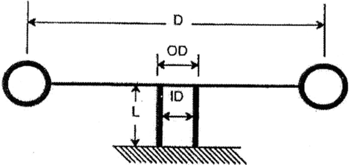
  Cross-sectional diagram of a torsional oscillator consisting of a torus supported by a hollow cylindrical tube acting as a torsional spring
  Full size image
  $$ {\mathrm{K}}_{ribbon}=G\frac{wh^3}{3L} $$
2. (b)
  Torsional resonance frequency. A mirrored galvanometer consists of a mirror and a current-sensing coil (see Fig. 2.7). The coil is suspended in a magnetic field produced by a permanent magnet structure by a ribbon of beryllium (Be) that is 100 μm thick, 2.0 mm wide, and 15 cm long. The shear modulus of beryllium is G_Be = 132 GPa. The moment of inertia of the mirror and coil is I_mirror = 3 × 10⁻⁸ kg-m². What is the natural frequency of torsional vibration?
3. (c)
  Noise. Using the Equipartition Theorem as discussed in Sect. 2.4.4, determine the root-means-squared angular displacement, $ {\theta}_{rns}=\sqrt{\left\langle {\theta}^2\right\rangle } $, of the mirror and coil at room temperature, T = 20 °C = 293 K.
5.
Cantilever springs. Consider a thin steel beam is 20.0 cm long, 2.0 cm wide, and 2.0 mm thick. Let Young’s modulus of the steel be E_Steel = 195 GPa. Assume that one end of the beam is rigidly clamped at x = 0, so (∂y/∂x)_x = 0 = 0, and a load of 1.0 kg is applied to the end at x = L = 20.0 cm.
1. (a)
  Uniform beam stiffness. By how much will the end of the beam be deflected from its equilibrium (straight) shape by the M = 1.0 kg load if g = 9.8 m/s²?
2. (b)
  Maximum stress and strain for the uniform beam. At what value of x is the stress in the beam largest? At what value of h, the distance from the beam’s neutral axis, is the stress largest at that value of x? What is the maximum strain and stress that is experienced by the loaded uniform beam?
3. (c)
  Triangular cantilever. What is the deflection of a similar cantilever spring, using the same amount of steel, which is also 20.0 cm long and is clamped at x = 0, but which has a base of w = 4.0 cm and the mass, M = 1.0 kg, is applied at the vertex of the triangle located at x = 20.0 cm?
4. (d)
  Maximum stress and strain for the triangular beam. At what value of x is the stress on the beam largest? At what value of h, the distance from the beam’s neutral axis, is the stress largest at that value of x? What is the maximum strain and stress that is experienced by the loaded triangular beam?
6.
Compression of a column. An aluminum rod has a length of 10.0 cm and a diameter of 5.0 mm. Assume Young’s modulus for aluminum is E_Al = 71 GPa.
1. (a)
  Compression. By how much will the beam be shortened if it is clamped at the bottom and a 5.0 kg mass is placed on the top?
2. (b)
  Buckling. How much mass would be required to cause such a beam buckle?
7.
Microphone vibration isolator. Figure 4.36 shows a piezoelectric microphone (Endevco Model 2510) on a (symmetrical) vibration mount that supports the microphone and its clamping fixture, attached to an aluminum base (5 × 1.5 × 0.4 cm) on two silicone rubber pads (1.5 × 1.5 × 0.5 cm). The rubber has a shear modulus of G = 350 kPa. The mass of the microphone and its mounting plate is 60 gm.
1. (a)
  Effective Young’s modulus. Using the dimensions of a single rubber pad in Fig. 4.36 and assuming β = 2.0, calculate the effective Young’s modulus, E_a, for compression.
2. (b)
  Compressional stiffness. Using the value of E_a, and the dimension of a single rubber pad in Fig. 4.36, calculate the compressional stiffness for a single pad.
3. (c)
  Natural frequency. Ignoring the counterweight below the mounting bracket that attaches to the Space Shuttle’s frame, calculate the microphone’s natural frequency of vibration for up and down motion.
4. (d)
  Shear vibration. The microphone can also undergo shear vibration. Calculate the shear stiffness provided by the two rubber pads and use that result to calculate the natural frequency for side-to-side vibration.
8.
Strain transformer. The cylindrical elastomeric mandrel shown in Fig. 4.37 is wrapped by a glass optical fiber and is capped at each end by rigid plates. The fiber is 80 μm in diameter and Young’s modulus of the glass is E = 62 GPa. Poisson’s ratio for the elastomer is ν = ½, so the rubber mandrel transforms compression of the mandrel into the lengthening of the optical fiber. The diameter of the cylinder is D = 3.98 cm, and the height is h = 1.92 cm. The mandrel is wrapped with N = 85 turns of optical fiber.
1. (a)
  Glass stiffness-length product. Based on Young’s modulus of glass and the diameter of the optical fiber, what is the stiffness-length product, Κ_glassL, of the fiber?
2. (b)
  Glass stiffness. Based on the diameter of the mandrel and the number of turns of optical fiber, what is the stiffness of the total length of fiber, Κ_fiber?
3. (c)
  Potential energy. The volume of the mandrel is V = πD²h/4. Keeping in mind that the elastomer is volume-conserving, since ν = ½, write the change in potential energy of the glass fiber for a change in the mandrel height, δh.
4. (d)
  Mandrel stiffness. Assuming that all of the compressional stiffness of the mandrel is due to the stretching of the glass fiber during compression, use your expression for the potential energy in part (c) to determine the effective stiffness of the mandrel.
5. (e)
  Moving mass. The mass density of the elastomer is ρ_2CN = 1020 kg/m³. If the displacement of the mandrel is linear with distance from the fixed end (like the Gerber scale of Fig. 2.2), what is the effective moving mass of the mandrel?
6. (f)
  Natural frequency. If one end of the mandrel is fixed and a proof mass, m_test = 100 gm, is placed on the other end, what is the natural frequency of vibration, f_o, if the contribution of the mandrel’s moving mass is included?

Notes

1.
For gases, this is an important distinction (e.g., the adiabatic bulk modulus of air is 40% larger than the isothermal bulk modulus). The difference between the adiabatic and isothermal Young’s modulus can be expressed in terms of the material’s absolute (kelvin) temperature, T; the (volumetric) coefficient of thermal expansion, α = (1/V) (∂V/∂T)_p; mass density, ρ; and specific heat (per unit mass) at constant pressure, c_p.
$$ {E}_{ad}=\frac{E_{iso}}{1-{E}_{iso}T{\alpha}^2/9\rho {c}_p} $$
In most solids, this is a small effect. At room temperature, E_isoTα ²/9ρ c_p is about 0.44% for aluminum and 340 ppm for copper.
2.
Simeon Denis Poisson (1781–1840).
3.
If the diameter of a sound beam is much greater than its wavelength, the associated compressions and expansions do not allow the material to “squeeze out” because there is a compression both above and below that is trying equally hard to squeeze the material in the transverse direction.
4.
In fluids, shearing forces diffuse; they are not restored elastically. See Sect. 9.4.
5.
The Lamé constants, λ and μ, also are taken as the two isotropic moduli in some elasticity calculations, although they are not listed in Table 4.1. The shear modulus, G, and μ are identical and $ \lambda =\frac{E\nu}{\left(1+\nu \right)\left(1-2\nu \right)}=\frac{G\left(E-2G\right)}{3G-E}=\frac{2 G\nu}{1-2\nu } $.
6.
I will apologize for indulging in a bit of a fraud at this point by introducing piezoelectric solids. So far, we have addressed the elastic behavior of isotropic solids that require only two independent moduli to completely specify their elastic behavior. Piezoelectric solids are intrinsically anisotropic crystalline materials that not only require more than two elastic constants but also require specification of the electrical impedance that provides the load across their electrodes, Z_load. For example, a piezoelectric material’s stiffness will be different if the electrodes are electrically shorted together (i.e., Z_load = 0) or left as an “open circuit” (i.e., Z_load = ∞). Anisotropic elasticity will be addressed later in this chapter (see Sect. 4.6), but for more complex crystalline substances, there are necessarily more than two independent elastic constants. In practice, once the relevant constants have been identified for a specific deformation, they are incorporated into Hooke’s law in the same way as the elastic constants of an isotropic solid.
7.
A ferroelectric ceramic behaves like a piezoelectric crystal. The difference is the piezoelectric behavior of the crystal is intrinsic, and a ferroelectric material (usually a ceramic or polymer) only exhibits piezoelectric behavior after the material has been “polarized,” usually by application of a large electric field at elevated temperatures [7].
8.
It is important to remember that in a textbook example, it is convenient to define “some generic steel,” but properties of steel (e.g., modulus, yield strength, endurance limit, heat capacity, thermal conductivity, electrical conductivity, etc.) vary with alloy composition and temper. In a commercial design, the choice of the material is very important.
9.
Tonpilz is from the German ton (tone) and pilz (mushroom). Apparently, the piezoelectric stack is the stem and the head mass is the “singing mushroom” cap.
10.
You will also want to employ some protective eyewear.
11.
The moment of inertia I = ∫ ρy²dA is related to the square of the radius-of-gyration since the radius-of-gyration is equivalent to I for a material of unit mass density, if divided by cross-sectional area S. The square of the radius-of-gyration is also equivalent to the second moment of area.
12.
In principle, the width could be kept constant and the thickness could be tapered so t(x) = [t(0)/L^1/3](L − x)^1/3. Since spring steel is available in constant thickness sheets, it is frequently more convenient to provide a linear taper of the width.
13.
The terms elastomeric and rubberlike will be used interchangeably in this chapter. While all rubbers are elastomers, not all elastomers are rubbers. The distinction is codified in the American Society for Testing and Materials (ASTM) Standard D 1566, which is based on the length of time required for a deformed sample to return to its shape after removal of the deforming force, as well as the extent of that recovery [26].
14.
In mathematics and signal processing the Kramers-Kronig relations are known as Sokhotski-Plemelj theorem or the Hilbert transform
15.
For an expression like that in Eq. (4.63), it is actually easier to solve for the minimum of the inverse than to solve for the maximum:
$$ \frac{d}{dx}\left(\frac{1+{x}^2}{x}\right)=\frac{d}{dx}\left(\frac{1}{x}+x\right)=0 $$
16.
The fact that these integrals are a consequence of linear response theory and causality can be proven by the use of complex integration of functions that are “analytic in the upper half-plane” and the Cauchy residue theorem.
17.
Carbon black (soot) is a common material that is mixed with rubber to increase its stiffness and strength. The shear modulus of natural rubber (latex) can increase by an order of magnitude if it is mixed with carbon black.
18.
Said another way, the molecular mobility is “frozen out.”
19.
Recall from Sect. 2.5.2 that decibel is defined in terms of a power or energy ratio (see Eq. 2.69). Since transmissibility, T, is a ratio of linear quantities, as defined in Eq. (2.96), it can be expressed as a decibel only when squared: dB = 10 log₁₀ T² = 20 log₁₀ T.
20.
An automotive valve spring in an engine that operates at 2000 rpm will be stressed 240 million times during the operational lifetime of 2000 h. A typical home refrigerator/freezer may last 15 years. (In America, refrigerators are replaced more often as an interior decorating choice than due to product failure.) If a refrigerator uses a spring that vibrates at 60 Hz, then the number of fully reversing stress cycles accumulated in 15 years of service would be 28 billion cycles if the compressor operated continuously.

References

L. D. Landau and E. M. Lifshitz, Theory of Elasticity, 2nd English edition (Pergamon, 1975). See pg. 17; ISBN 0 08 006465 5
Google Scholar
G.G. Marquez, One Hundred Years of Solitude (Harper Collins, New York, 2003); ISBN 0-19-515544-4
Google Scholar
E.H. Love, A Treatise on the Mathematical Theory of Elasticity, 4th edn. (Dover reprint, 1944); ISBN 0-486-60172-9
Google Scholar
R.S. Lakes, Foam structures with a negative Poisson’s ratio. Science 235(4792), 1038–1040 (1987)
Article ADS Google Scholar
S. R. Lampman (ed.), ASM Handbook, Vol. 19 – Fatigue and Fracture (ASM International, Metals Park, 1996); ISBN 0-87170-385-8
Google Scholar
J.E. Shigley, C.R. Mischke, Mechanical Engineering Design, 5th edn. (McGraw-Hill, Boston, 1989); ISBN 0-07-056899-5
Google Scholar
O.B. Wilson, Introduction to Theory and Design of Sonar Transducers (Peninsula, Los Altos, 1988)
Google Scholar
S. L. Ehrlich and A. F. Medeiros, Wide band transducer, U. S. Patent No. 3,860,901 (January 14, 1975)
Google Scholar
D. Boucher, Process to increase the power of the low frequency electro acoustic transducers and corresponding transducers, US Patent No. 5,070486 (December 3, 1991)
Google Scholar
L.D. Landau, E.M. Lifshitz, Mechanics (Pergamon, Oxford, 1960). See §24
MATH Google Scholar
M.E. Poese, R.M. Keolian, R.W.M. Smith, E. Mitchell, S.L. Garrett, Performance estimates for a helium-based thermoacoustic Stirling chiller. Int. J. Low Carbon Technol. 8, 79–84 (2013)
Article Google Scholar
W.C. Young, R.G. Budynas, Roark’s Formulas for Stress and Strain, 7th edn. (McGraw-Hill, New York, 2002); ISBN 0-07-072542-X
Google Scholar
S. L. Garrett, R. M. Keolian and R. W. M. Smith, High-efficiency moving magnet loudspeaker,” U. S. Patent No. 6,307,287 (October 23, 2001)
Google Scholar
J. Liu, S. Garrett, Characterization of a small moving-magnet electrodynamic linear motor for use in a thermoacoustic refrigerator. J. Acoust. Soc. Am. 118(4), 2289–2295 (2005)
Article ADS Google Scholar
H.E. Boyer, T.L. Gall, Metals Handbook: Desk Edition (American Society for Metals, Metals Park, 1985); ISBN 0-81170-188-X
Google Scholar
S. L. Garrett, Cylindrical spring with integral gas seal, US Patent No. 6,755,027 (June 29, 2004)
Google Scholar
EJMA, Standards of the Expansion Joint Manufacturers Association, 10th edn. (EJMA, Tarrytown, 2017)
Google Scholar
H. Cavendish, Experiments to determine the Density of the Earth. Philos. Trans. R. Soc. Lond. Part II 88, 469–526 (1798)
Google Scholar
C.J. Ancker Jr., J.N. Goodier, Pitch and curvature correction for Helical Springs. ASME J. Appl. Mech. 25(4), 471–483 (1958)
MATH Google Scholar
M. Wahl, Mechanical Springs, 2nd edn. (McGraw-Hill, New York, 1963)
Google Scholar
L.R. Wilberforce, On the vibrations of a loaded spiral spring. Philos. Mag. 38, 386–392 (1896)
Article Google Scholar
R.E. Berg, T.S. Marshall, Wilberforce oscillations and normal modes. Am. J. Phys. 56(1), 32–38 (1991)
Article ADS MathSciNet Google Scholar
A. Sommerfeld, Mechanics of Deformable Bodies: Lectures on Theoretical Physics, vol II (Academic, New York, 1950), pp. 308–314
MATH Google Scholar
N. Feather, Vibration and Waves (Penguin, London, 1964), pp. 59–67
Google Scholar
J. Wilhelm, K.A. Gillis, J.B. Mehl, M.R. Moldover, An improved Greenspan acoustic viscometer. Int. J. Thermophys. 21, 983–999 (2000)
Article Google Scholar
R. N. Capps, Elastomeric Materials for Acoustical Applications (Naval Research Laboratory, Underwater Sound Reference Detachment, 15 September 1989)
Google Scholar
L.D. Landau, E.M. Lifshitz, Statistical Physics, 2nd edn. (Addison-Wesley, Reading, 1969), pp. 384–391, See §125; ISBN 0-201-04167-7
Google Scholar
L.D. Landau, E.M. Lifshitz, Electrodynamics of Continuous Media (Pergamon, London, 1960); ISBN 0-08-09105-9. §62
Google Scholar
B. Bhatia, Ultrasonic Absorption: An Introduction to the Theory of Sound Absorption and Dispersion in Gases, Liquids, and Solids (Oxford, 1967). Reprinted (Dover, 1985); ISBN 0-486-64917-2
Google Scholar
H. Bode, Relations between attenuation and phase in feedback amplifier design. Bell Syst. Tech. J. 19, 421 (1940)
Article Google Scholar
V. Mangulis, Kramers-Kronig or dispersion relations in acoustics. J. Acoust. Soc. Am. 36, 211–212 (1964).; Relation between the radiation impedance, pressure in the far field, and baffle impedance, J. Acoust. Soc. Am. 36, 212–213 (1964)
Article ADS Google Scholar
S. Garrett, S. Adams, S. Putterman, I. Rudnick, Resonant nonlinear mode conversion in He II. Phys. Rev. Lett. 41(6), 413–416 (1978)
Article ADS Google Scholar
R. Kronig, H.A. Kramers, Absorption and dispersion in X-rays spectra. Z. Phys. 48, 174 (1928)
Article ADS Google Scholar
J. W. Strutt (Lord Rayleigh), The Theory of Sound, vol I, 2nd edn. (Macmillan, London, 1894), p. 153; Reprinted (Dover, 1945); ISBN 486-60292-3
Google Scholar
M. O’Donnell, E.T. Jaynes, J.G. Miller, Kramers-Kronig relationships between ultrasonic attenuation and phase velocity. J. Acoust. Soc. Am. 69(3), 696–701 (1981)
Article ADS Google Scholar
C.M. Harris, A.G. Piersol, Harris’ Shock and Vibration Handbook, 5th edn. (McGraw-Hill, New York, 2002); ISBN 0-07-137081-1
Google Scholar
W. Nolle, Dynamical mechanical properties of rubberlike materials. J. Polym. Sci. 5(1), 1–54 (1950)
Article ADS Google Scholar
J.D. Ferry, Viscoelastic Properties of Polymers, 3rd edn. (Wiley, New York, 1980.; ISBN: 978-0-471-04894-7
Google Scholar
J.C. Snowdon, Vibration and Shock in Damped Mechanical Systems (Wiley, New York, 1968)
Google Scholar
L. D. Landau and E. M. Lifshitz, Theory of Elasticity, 2nd English edition (Pergamon, 1975). §10, see pp. 41–42ISBN 0 08 006465 5
Google Scholar
H. Ledbetter, Chapter 11: Monocrystal-polycrystal elastic-constant models, in Handbook of Elastic Properties of Solids, Liquids, and Gases: Vol. III – Elastic Properties of Solids: Biological and Organic Materials, Earth and Marine Sciences, ed. by M. Levy, H. Bass, R. Stern, (Academic, 2000). ISBN 0-12-445763-0
Google Scholar
W.G. Cady, Piezoelectricity (McGraw-Hill, New York/London, 1946)
Google Scholar
S. L. Garrett, Torsionally resonant toroidal thermoacoustic refrigerator,” U.S. Patent No. 5,953,921 (September 21, 1999)
Google Scholar
C. D. Stehle, Vibration isolation of a microphone, U.S. Defense Technical Report No. AD A 161 018 (October 1985)
Google Scholar
D.L. Gardner, T. Hofler, S.R. Baker, R.K. Yarber, S.L. Garrett, A fiber-optic interferometric seismometer. J. Lightwave Technol. 5(7), 953–960 (1987)
Article ADS Google Scholar

Download references

Author information

Authors and Affiliations

Pine Grove Mills, PA, USA
Steven L. Garrett

Authors

Steven L. Garrett
View author publications
You can also search for this author in PubMed Google Scholar

Rights and permissions

Open Access This chapter is licensed under the terms of the Creative Commons Attribution 4.0 International License (http://creativecommons.org/licenses/by/4.0/), which permits use, sharing, adaptation, distribution and reproduction in any medium or format, as long as you give appropriate credit to the original author(s) and the source, provide a link to the Creative Commons license and indicate if changes were made.

The images or other third party material in this chapter are included in the chapter's Creative Commons license, unless indicated otherwise in a credit line to the material. If material is not included in the chapter's Creative Commons license and your intended use is not permitted by statutory regulation or exceeds the permitted use, you will need to obtain permission directly from the copyright holder.

Reprints and permissions

Copyright information

About this chapter

Cite this chapter

Garrett, S.L. (2020). Elasticity of Solids. In: Understanding Acoustics. Graduate Texts in Physics. Springer, Cham. https://doi.org/10.1007/978-3-030-44787-8_4

Download citation

DOI: https://doi.org/10.1007/978-3-030-44787-8_4
Published: 03 November 2020
Publisher Name: Springer, Cham
Print ISBN: 978-3-030-44786-1
Online ISBN: 978-3-030-44787-8
eBook Packages: Physics and AstronomyPhysics and Astronomy (R0)

Publish with us

Policies and ethics