
Abstract
The vibrating string has been employed by nearly every human culture to create musical instruments. Although the musical application has attracted the attention of mathematical and scientific analysts since the time of Pythagoras (570 BC–495 BC), we will study the string primarily because its vibrations are easy to visualize and string vibrations introduce concepts and techniques that will recur throughout our study of the vibration and the acoustics of continua. In this chapter, we will develop continuous mathematical functions of position and time that describe the shape of the entire string. The amplitude of such functions will describe the transverse displacement from equilibrium, y(x, t), at all positions along the string. The importance of boundary conditions at the ends of strings will be emphasized, and techniques to accommodate both ideal and “imperfect” boundary conditions will be introduced. Solutions that result in all parts of the string oscillating at the same frequency which satisfy the boundary conditions are called normal modes, and the calculation of those normal mode frequencies will be a focus of this chapter.
You have full access to this open access chapter, Download chapter PDF
Keywords
The vibrating string has been employed by nearly every human culture to create musical instruments. Although the musical application has attracted the attention of mathematical and scientific analysts since the time of Pythagoras (570 BC–495 BC), we will study the string because its vibrations are easy to visualize and it introduces concepts and techniques that will recur throughout our study of vibration and the acoustics of continua. A retrospective of these concepts and techniques is provided in Sect. 3.9, near the end of this chapter. You might want to skip ahead to read that section to understand the plot before you meet the characters.
In the analyses of the previous chapter, we sought equations that would specify the time histories, x (t), of the displacement of discrete masses constrained to move only along one dimension, focusing particularly on single-frequency time-harmonic motion. At the end of that chapter, we examined the limit as the number of masses became infinite and the inter-mass spacing decreased in a way that held constant the linear mass density, ρL, of our “string of pearls” in Sect. 2.7.7. In this chapter, we will develop continuous mathematical functions of position and time that describe the shape of the entire string. The amplitude of such functions will describe the transverse displacement from equilibrium, y(x, t), at all positions along the string.Footnote 1
1 Waves on a Flexible String
We begin this exploration, as we did with the simple harmonic oscillator, by seeking an equation-of-state (i.e., a relationship between forces and displacements), but now we will examine an infinitesimal segment of string, with length, dx, acted upon by the tension applied at both ends. As we did with the “string of pearls” in Sect. 2.7.7, we will assume that the string has a constant linear mass density, ρL, and that the string has no flexural rigidity (i.e., no bending stiffness); thus the string can only apply forces produced by the tension, Τ, to influence the string’s motion. We will also assume that the string’s displacements from equilibrium are small enough that the displacements create length changes that only contribute modifications to the tension that are second-order in the ratio (y/L), as shown in Eq. (2.129), and can be neglected in a linear (i.e., first-order) analysis.
Figure 3.1 shows the infinitesimal length of string as just described. It is acted upon by the vertical components of the tension at either end, Fv (x) and Fv (x + dx). As will be demonstrated, if the string does not have any curvature, there will be no net transverse force. We can apply Newton’s Second Law to that segment of length, dx, once we calculate the net transverse force, dFnet.
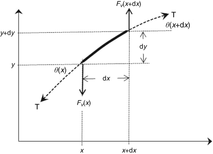
An infinitesimal length, \( ds=\sqrt{dx^2+{dy}^2}\cong dx \), of a string with uniform linear mass density, ρL, that is acted upon by the tension, Τ, exerting a force along the direction of the string. The angle that the string makes with the horizontal at x is θ(x), and the angle at x + dx is θ(x + dx). If these angles are different, there will be a net transverse force on that segment, causing it to accelerate
Since x, y, and t are all independent variables, partial derivatives are used to remind us to hold the other two variables constant when we take a derivative with respect to the third variable.
This approximate expression utilizes the first two terms in the Taylor series of Eq. (1.2). After cancellation of the two leading (Τ sin θ)x terms of opposite sign, we are left with an expression for the net transverse force that can be expanded by the product rule of Eq. (1.10).
We have again imposed the assumption that ∂y/∂x ≪ 1, so sin θ ≅ tan θ ≅ dy/dx, where these two differential lengths, dx and dy, are shown in Fig. 3.1.Footnote 2 For now, we will assume that the tension along the string is independent of position, so ∂Τ/∂x = 0, although we will reconsider this restriction later in Sect. 3.4.3, when we consider the oscillations of a heavy chain that has a tension that decreases as we recede from its point of suspension (since the lower links are supporting less mass than the upper links).
For our simplified case, our equivalent of an equation-of-state for the string shows that the net transverse force, dFv, on an infinitesimal string segment is the product of the constant tension, Τ, and the curvature of the string.Footnote 3 This is consistent with our intuition. Strings that are displaced but remain straight, like those strings attached to the discrete masses shown in Figs. (2.23) through (2.26), only apply forces at the “kinks” produced at the positions of the discrete masses or at the fixed boundaries.
Once again, we will use Newton’s Second Law to provide the dynamical equation that describes the acceleration of that infinitesimal string segment with mass, ρL dx, acted upon by dFnet.
After cancellation of the common differential, this solution is written in a form known as the wave equation where we identify the speed of transverses waves, \( c=\sqrt{\mathrm{T}/{\rho}_L} \).
Such a second-order homogeneous partial differential equation must have two independent solutions. As demonstrated below, those solutions can have any functional form so long as the arguments of those functions only involve two particular combinations of the space and time coordinates.
At this point, the form of the two functions, f− and f+, is entirely arbitrary, but the requirement imposed by the wave equation suggests that after some time t, f− (x − ct) will be identical to its shape at t = 0, except at a distance, x = ct, farther to the right. Similarly, f+ (x + ct) will be identical to its shape at t = 0, except at distance, x = −ct, farther to the left. Because these functions propagate with speed, c, f− (x − ct) and f+ (x + ct) are called traveling wave solutions.
The wave equation can be written in a “linear operator” form (see Sect. 1.3) represented by the d’Alembertian operator.
In the lower expression, the operator has been factored to make it easy to see that the solutions shown in Eq. (3.5) satisfy the wave equation one or the other term in the rightmost version of Eq. (3.6) vanish.
The proof that Eq. (3.5) is a solution to the wave equation of Eq. (3.4) or Eq. (3.6) is simplified by the introduction of a new variable, w± = x ± ct, and the use of the chain rule.
The same transformation can be applied to the partial derivative with respect to time.
Substituting Eqs. (3.7) and (3.8) into the factored version of Eq. (3.6) shows that f− makes the operator, W, with the sum identically zero.
Since the second operator is now identically zero, the first operator has no effect. Since the order of application of the factored linear (differential) operators is irrelevant, we could apply the operator with the minus sign to f+ to obtain the same result. The factorization of the second-order partial differential equation we called the wave equation in Eq. (3.4) into the product of two one-way first-order linear differential operators can be useful in problems where the propagation is only in one direction (i.e., for situations where there is no reflected wave).
The validity of the solutions in Eq. (3.5) to the wave equation in Eq. (3.4) can be established directly by calculation of the second partial derivative with respect to position, x, or with respect to time, t, produced by a second application of the chain rule.
In the limit of small displacements, it is important to appreciate that any disturbance will propagate along the string at a constant speed forever without reducing its amplitude or changing shape. That would not be true if our analysis had incorporated dissipation or if nonlinear (i.e., second-order) contributions had not been suppressed.
The result would have been identical if we had chosen to exchange the order of the space and time coordinates. The reader should be convinced that replacing the solution in Eq. (3.5) by the form in Eq. (3.12) still satisfies Eq. (3.4) or Eq. (3.6).
The function with the minus sign in its argument still corresponds to a right-going wave, and the plus sign corresponds to the left-going wave. As will be shown later in this chapter, the choice of Eq. (3.12) or of Eq. (3.5) might simplify a particular calculation.
Figure 3.2 illustrates the propagation of a Gaussian pulse with the form of Eq. (1.87) but with an argument which is proportional to x ± ct.
For Fig. 3.2, I have chosen the right-going argument, x − ct. The upper plot of Fig. 3.2 captures the pulse at an instant, t1, with the pulse centered at x1. The lower plot shows the same pulse at a later instant, t2, after the center of the pulse had advanced to x2. Over that time interval, Δt = t2 − t1, all portions of the pulse have advanced by a distance, Δx = x2 − x1. The speed of such a transverse disturbance, whatever the shape, is defined by the usual kinematic relation: c = Δx/Δt.

(Above) A Gaussian pulse with displacement, y (x, t), given by Eq. (3.13), is propagating to the right. The pulse is shown at an instant, t1, where it has its maximum displacement centered at position, x1. (Below) At a later time, t2 > t1, the center of the pulse has moved to a new position, x2. The change in position is related to the change in time by the speed of transverse waves on a string of uniform linear mass density, ρL, and uniform tension, Τ, \( c=\sqrt{\mathrm{T}/{\rho}_L}\Rightarrow\ \left({x}_2-{x}_1\right)=c\left({t}_2-{t}_1\right) \)
2 Pulse Reflections at a Boundary and the Utility of Phantoms
Infinite strings are hard to come by, and a method for applying a uniform tension to such a beast is even harder to imagine. A string of finite length will be terminated by two boundaries. To initiate our analysis of the reflection of a pulse from such a boundary, we will examine two limiting cases: A rigid (“fixed”) boundary will suppress the transverse motion of the string by providing whatever vertical force, Fv = −T sin (θ) ≅ −T(∂y/∂x)boundary, that would be required to keep the string’s attachment point immobile.Footnote 4 The opposite limit is a free boundary. Such a termination will maintain the tension in the string but will allow the end of the string to move up or down without constraint. Footnote 5 Since no vertical forces are produced by the boundary, the pulse must arrive at such a free boundary and leave without any slope, Fy = Τ(∂y/∂x)boundary = 0. The common “textbook” way to envision such a boundary is to picture the string attached to a massless ring that slides along a frictionless pole.
Of course, these are only idealized limits that simplify calculations and help to develop our intuition. (If the bridge on a guitar or violin did not move, then the body would not radiate sound.) In this chapter, we will be able to analyze the consequences of a broad range of termination conditions that may be massive (e.g., a mass at the end of a pendulum), elastic (e.g., a string attached to a flexible cantilevered beam), resistive (e.g., a string tensioned by our massless ring but with the ring connected to a dashpot), or a combination of all three.
We will begin by analyzing a pulse that is impinging upon a rigid boundary. This situation is shown schematically in Fig. 3.3 for a Gaussian pulse of the same kind that was displayed in Fig. 3.2. The point of rigid attachment is indicated by the hatched barrier located at x = 0. At that boundary, y (0, t) = 0 for all times. We also know that the linearity of our general solution to the homogeneous wave equation, given in Eq. (3.5) or Eq. (3.12), allows superposition of any number of such right- and left-going pulses that may be required to satisfy the initial conditions or the boundary constraints.

The positive Gaussian pulse (solid line) at the far left is shown approaching a rigid boundary at x = 0, represented by the hatched rectangle. To satisfy the fixed boundary condition, y (0, t) = 0, an inverted phantom (dashed line), shown at the far right, is launched along an imaginary extension of the string. The phantom is approaching the boundary from an equal distance, but propagating in the opposite direction, as indicated by the dashed arrow below the phantom pulse. The superposition of those two pulses (dotted line) makes y (0, t) = 0. As the two pulses leave the boundary, the phantom propagates along the actual string, and the original pulse becomes the phantom
One fact that is not intuitively obvious is that we can choose to imagine the string extending beyond the termination, as long as the superposition of the pulses coming from that nonexistent extension can be combined with pulses on the physical portion of the string to satisfy the requirements imposed at the boundary. In Fig. 3.3, the pulse at the extreme left, with the arrow above pointing to the right, indicates the real pulse on the real string that is approaching the boundary at x = 0. We will satisfy the boundary condition, y (0, t) = 0, by imagining a pulse that is identical to that initial pulse but inverted, approaching from an equal distance behind the boundary. That phantom is shown at the extreme right with a dashed line and a dashed arrow below it. Both pulses are propagating at the transverse wave speed, c, although in opposite directions.
Since the real pulse and the phantom are always equidistant from the boundary, they reach it at the same time and superimpose linearly within their regions of overlap. One instant during that overlapping time interval is illustrated in the vicinity of the boundary in Fig. 3.3 by the dotted line. At that instant, the “real” pulse has started to excite the nonexistent portion of the string, and the phantom has started to appear on the real string. Because of the equality of their amplitude and the congruency of their shape, at x = 0 their sum, indicated by the dotted line, will be zero. At the instant during overlap, shown in Fig. 3.3, the sum exhibits a greater slope and decreased amplitude. We have assumed an infinitely rigid termination, so the vertical force, Fy(x, t) = − Τ(∂y/∂x)x = 0, required to immobilize the string at the boundary, is available to enforce the complete immobilization.
At the instant the two pulses completely overlap, their superposition will mean that the real string (and the fictitious extension) will be flat everywhere. Subsequently, the vertical force which immobilized the string at the boundary will launch the inverted pulse traveling in the opposite direction in the real portion of the string. At a later time, the inverted pulse is shown propagating away from the barrier along the real string, and the original pulse has crossed the barrier and has become the phantom.
We should pause momentarily to reflect (no pun intended) on the process that was used to satisfy the conditions at the real string’s rigid termination. The invention of the phantom provided a simple method to satisfy the boundary condition by trading a semi-infinite string for an infinitely long one. We should remember that there are only real strings and real forces. On the other hand, we would be remiss if we did not also marvel at the human imagination and intelligence that produced such a simple way to understand such a complex combination of wave–barrier interactions.
It is easy to repeat this analysis for the other limiting case, a boundary that applies no vertical forces on the string. In that case, we require that the slope of the pulse vanishes for all times at x = 0 (i.e., −Τ(∂y/∂x)x = 0 = 0). Figure 3.4 is identical to Fig. 3.3 except that the phantom is not inverted. Near the region of the boundary, where the pulses overlap, their superposition always maintains zero slope. At the exact instant of overlap, the pulse has twice its original amplitude.

The positive Gaussian pulse (solid line) at the far left is shown approaching a force-free boundary at x = 0, represented by the hatched rectangle. To satisfy the boundary condition, (∂y/∂x)x = 0 = 0, a phantom (dashed line), shown at the far right, is launched along an imaginary extension of the string, approaching the boundary from an equal distance, but propagating in the opposite direction. The superposition of those two pulses (dotted line) maintains the slope of their sum to be zero at x = 0 and doubles their amplitude at the instant of complete overlap. As the two pulses leave the boundary, the phantom propagates along the actual string, and the original pulse becomes the phantom
This approach to the solution of boundary-value problems is common in acoustics and other fields of physics (e.g., electrostatics, optics). It is known as the method of images. When we study sound sources in near boundaries (see Sect. 12.4.1 and Figs. 12.13 and 12.14) or in rooms (see Sect. 13.1.1), or underwater in proximity to an air–water interface, we will sprinkle image sources about in regions that are outside those spaces that are physically accessible to the waves to satisfy boundary conditions.
The same results, for both the fixed and free boundaries, can be expressed mathematically by the appropriate choice of functions, with w± in their arguments. If we again choose a Gaussian pulse and abbreviate the waveform of Eq. (3.13) as y(x, t) = G±(x ± ct), then the rigid boundary condition at x = 0 is satisfied by a solution y(x, t) = G−(x – ct) – G+(x + ct). With the additional restriction that when x ≤ 0, we need not concern ourselves with the nonexistent portions of the string.
To satisfy the free boundary condition, we require that the slope vanishes at the boundary x = 0.
Evaluation of those expressions at x = 0, with w− = −ct and w+ = ct, leads to the requirement that both G− and G+ be positive pulses.
3 Normal Modes and Standing Waves
We will now examine the free vibrations of a uniform string of length, L, and will start by rigidly fixing both ends of the string so that y (0, t) = y (L, t) = 0. Those boundary conditions would provide a close approximation to a guitar, violin, erhu (二胡), sitar (सितार), harp, ukulele, Balkan tambura, or piano string. Recalling that a normal mode is a particular displacement that results in all parts of the system oscillating at a single frequency, we will seek the normal mode vibration frequencies for a uniform string by again assuming a right- and left-going solution to the wave equation and then combining those solutions in a way that satisfies both boundary conditions simultaneously. This will produce a theoretically infinite set of normal mode frequencies. It should come as no surprise that the mode shapes for the lower-frequency modes will resemble the lower-frequency modes of our “string of pearls” that were diagrammed in Fig. 2.30.
The solutions to the wave equation provided in Eq. (3.5) or Eq. (3.12) involve arguments that have the dimensions of length. The arguments of any mathematical function (e.g., sines, cosines, or exponentials) must be dimensionless. To provide dimensionless arguments that simplify our mathematics, we will scale the argument of the wave functions by a scalar constant, k, which has the dimensions of an inverse length [m−1] that is known as the wavenumber.
As before, the minus sign indicates propagation in the direction of increasing x (to the right), and the plus sign corresponds to propagation in the direction of decreasing x (to the left). The rightmost version of Eq. (3.15) imposes the requirement that kc = ω. Since we seek time-harmonic normal modes at radian frequency, ω = 2πf, we can choose either a complex exponential or a sinusoidal expression as our function of the (now dimensionless) argument required of solutions to the linear wave equation.
These solutions are periodic in both space and time. We can define the wavelength, λ, of the disturbance that propagates to the right along the string as y(x, t) = y(x + nλ, t), where n can be any positive or negative integer or zero. Based on that definition, the wavelength can be related to the wavenumber.
Similarly, y(x, t) = y(x, t + nT), where T = (1/f) = (2π/ω) is the period of the oscillation. Fig. 3.5 illustrates the propagation of the harmonic (i.e., single frequency) disturbance along the string as a function of both position and time.

A time-harmonic wave that propagates to the right along a uniform string. (Above) The solid line is the wave at time, t1, and the dashed line is the same wave at slightly later time, t2 > t1. The distance between successive peaks or troughs is the wavelength, λ = (2π/k), where k is the wavenumber. (Below) The solid line is the time history of a wave passing a point, x1, and the dashed line is the same wave passing a point, x2 > x1, that is farther to the right. The wave repeats itself after a time, T = (1/f) = (2π/ω), that is, the period of the harmonic disturbance. The unit of frequency, f, is given in hertz [Hz], and the unit of angular frequency, ω, is in radian/second [rad/s] or just [s−1]
3.1 Idealized Boundary Conditions
Our experience with the reflection of pulses from fixed and free boundaries in Sect. 3.2 suggests that we will be able to satisfy the boundary conditions on this string by superposition of left- and right-going waves and letting the displacement amplitude, y(x, t), be a complex function of x and t.
The boundary condition at x = 0 is |y(0, t)| = 0. Evaluation of this restriction on Eq. (3.18) requires that A = −B.
In this expression, we have used the fact that 2j sin x = (ejx − e−jx) and have absorbed 2jB into the new complex amplitude constant (phasor), \( \hat{\mathbf{C}} \).Footnote 6 The imposition of the boundary condition at x = 0 has provided a rather satisfying form for our solution since sin(0) = 0, as required.
The imposition of the boundary condition at x = L now produces the quantization of the frequencies that represent the normal modes of the fixed-fixed string. To make |y(L, t)| = 0, only those discrete values of kn that make sin knL = 0 will satisfy this second boundary condition.
The physical interpretation of this result is simple: the normal mode shapes of a uniform fixed-fixed string correspond to placing n sinusoidal half-wavelengths within the overall length, L, of the string. Substitution of these normal mode frequencies, ωn, and wavenumbers, kn, into the functional form of Eq. (3.19) provides the description of the mode shapes, yn (x, t), for each of the normal modes.
These solutions are called standing waves. It is worthwhile to remember that these standing waves are equivalent to the superposition of two counter-propagating traveling waves of equal amplitude that were our starting point in Eq. (3.18). The term “standing wave” refers to the fact that the amplitude envelope is fixed in space (i.e., standing), although the transverse displacement varies sinusoidally in time. The locations where the sin knx term vanishes are called the displacement nodes (or just nodes) of the standing wave. In this case, there are always two nodes located at the rigid boundaries. As the mode number, n, increases, (n – 1) additional nodes appear along the string and are equally spaced from each other for a string of uniform mass density and constant tension.
The locations where sin kn x = 1 are designated anti-nodes and are the location of the largest amplitudes of harmonic motion. Those anti-nodes are equidistant from the nodes for a string of uniform density and tension. The separation distance of adjacent nodes and anti-nodes for a uniform string is λn/4.
This result also accounts for the ubiquity of musical instruments that are based on the tones produced by the vibrations of a fixed-fixed string.
The lowest-frequency mode, n = 1, is known as the fundamental frequency, f1 = c/2L. The higher normal mode frequencies are known as the overtones. The second mode, f2 = c/L, is called the “first overtone.” I find this “overtone” terminology to be needlessly confusing and do not use it in this textbook.
The frequencies in Eq. (3.22) form a harmonic series. The frequency of each normal mode is an integer multiple of the fundamental mode: fn = nf1. Pythagoras recognized the intervals produced by a string that was shortened by ratios of integers produced tonal combinations that were pleasing to the ear. A string whose length was halved produced the same note as the full-length string but one octave higher in frequency. A string that is one-third as long as the original produces a note that is a “perfect fifth” above the octave. (See Table 3.1 for the frequency ratios of musical frequency intervals.) Keeping the string length constant but fitting integer numbers of half-wavelengths into the string produces the same frequency as the fundamental of the shorter string.
Although I know of no physical manifestation for the normal modes of a fixed-free string (unless the mass of the string provides its tension, as for the “heavy chain” in Sect. 3.4.3),5 it is easy to calculate those normal mode frequencies. Those frequencies will provide some useful insights that are applicable to acoustic resonators or vibrating bars.Footnote 7 Leaving the boundary condition at x = 0 fixed, so y (0, t) = 0, we can start with Eq. (3.19). Since the end at x = L is free, (∂y/∂x)x = L = 0. This second condition again quantizes the values of kn that simultaneously satisfy both boundary conditions.
This can only be satisfied for all times if cos kn L = 0.
Again, the simple interpretation is that odd-integer multiples of one-quarter wavelengths are fit within the overall length of the fixed-free string of length L. This produces a harmonic series that includes only odd-integer multiples of the fundamental, f1 = c/4 L, f2 = 3c/4 L, f3 = 5c/4 L, etc.
3.2 Consonance and Dissonance*
“Agreeable consonances are pairs of tones which strike the ear with a certain regularity; this regularity consists in the fact that the pulses delivered by the two tones, in the same time, shall be commensurable in number, so as not to keep the eardrum in perpetual torment.” Galileo Galilei, 1638 [1]
The perception of musical (and nonmusical) tones has been an interesting topic for experimental psychologists long before the term “experimental psychologist” came into existence. A perceptual feature of hearing that seems to span many cultures is that of the consonance or dissonance when two notes with different fundamental frequencies are presented simultaneously to a listener. The ratio of the frequency of the higher-frequency tone to the frequency of the lower-frequency tone is known as the interval between the two notes. The intervals that are judged to be “harmonious” are called consonant, while other ratios are judged to be “annoying” (producing “perpetual torment”) or dissonant. Table 3.1 lists several consonant frequency intervals and the “musical” designation of that interval (e.g., octave, perfect fourth, minor third, etc.).
A harmonic series is not produced for a nonuniform string or for a uniform string subject to nonuniform tension (e.g., a hanging chain), or a uniform string that has some stiffness (in addition to the restoring force provided by the tension, as discussed in Sect. 5.5), or a uniform string subject to boundary conditions that are not perfectly rigid or perfectly free (see Sect. 3.6).
There are various physical explanations for humans finding some intervals pleasing (consonant) and others unpleasant (dissonant), but a few simple arguments can be based upon the relationships between the harmonics of the two tones either being identical, or creating a consonant interval, or being separated by a sufficient frequency difference that the superposition of the overtones do not produce perceptible beating (i.e., a high rate of amplitude modulation due to the interference between the two tones).
Helmholtz concluded that dissonance occurred when the difference between any overtones of the two tones produced between 30 and 40 beats per second [2]. Later investigations have shown that the dissonance caused by the beat rate will depend upon frequency [3]. Table 3.2 lists a series of harmonics that start with “Concert A4,” a frequency defined as 440 Hz. A4 = 440 Hz is used to set the tuning of pitch for most Western musical instruments. As can be seen, the overtones for a single string produce mostly octaves and perfect fifths.
3.3 Consonant Triads and Musical Scales*
As we have just seen, the normal modes of a perfect string generate a harmonic series with relationships that are mostly judged to be pleasing to the ear (i.e., consonant). That is a good start, but music is made by a succession of notes that produce a melody within some rhythmic (i.e., temporal) structure. The construction of a series of musical notes (i.e., a musical scale) that is also pleasant is rather complicated. It is possible to construct a musical scale, suitable for Western music (as well as country music), which is based on the consonant intervals in Table 3.1. As will be illustrated briefly [4], it is not possible to create such scales for which all intervals are consonant and which can be readily transposed so that a melody which is written in a particular key signature (i.e., based on a scale that starts on a specific note) can be played in some other key. A compromise that has been found acceptable, called the scale of equal temperament (also known as the tempered scale), places 12 semitones within an octave, all of which that have a constant frequency ratio of 21/12 = 1.05946.
A musical scale that has eight notes within an octave can be constructed based on three major triads. Such a scale is called the scale of just intonation. As seen in Table 3.2, a three-note major chord is built from a minor third (6:5) above a major third (5:4), producing a frequency ratio of 4:5:6 that is perceived to have a particularly pleasant sound. Those of you familiar with American blues and rock music will recognize that many melodies are based on a succession of three such major chords based on a first (root) note, the perfect fourth, and the perfect fifth. These are known as the tonic (I chord), the subdominant (IV chord), and the dominant (V chord).
If we choose C as our root, then the tonic is {C, E, G}. The dominant (V) major chord is built on the perfect fifth G to produce {G, B, D}, thus introducing B as a major third above the perfect fifth, (5/4)(3/2) = 15:8, and D which is a perfect fifth above a perfect fifth, (3/2)(3/2) = 9/4. Reducing the frequency of D by an octave places it within the original octave where we are building the scale, thus producing the interval 9:8, known as a major whole tone. The process is repeated one last time for the subdominant (IV) chord rooted on the perfect fourth, {F, A, C}. A is a major third above a perfect fourth (5/4)(4/3) = 5:3, and C is the octave. The intervals between the notes and the root, as well as the intervals between adjacent notes, are shown in Table 3.3.
The scale of just intonation introduces two other triads with frequency ratios of 10:12:15 that are known as minor triads. Like the major triad, they are constructed from a major third (5:4) and a minor third (6:5), but with the major third above the minor third.
It all sounds good until we examine two of the new fifths that were generated in this process. Five of the fifths are perfect: G:C = B:E = C:F = D:G = E:A = 3:2, but the ratio of B:F is not actually a fifth, B:F = (8/3)/(15/8) = (64/45) = 1.422 ≠ 3:2 = 1.500. Similarly D:A which should be a fifth is D:A = (10/3)/(18/8) = (40/27) = 1.481 ≠ 3:2 = 1.500. Examination of the perfect fourth reveals two more problematic intervals. Again, five of the fourths are perfect: F:C = G:D = A:E = C:G = E:B = 4:3 = 1.333, but two are not. F:B = (15/8)/(4/3) = 45:32 = 1.406 ≠ 1.333 and D:A = (18/8)/(5/3) = 27:20 = 1.350 ≠ 1.333.
If we try to construct a major triad other than I, IV, and V, used to produce the just scale, we see that sharps and flats must be added that correspond to the “black keys” on a piano. Those sharps and flats do not necessarily have the same frequencies. For example, if we construct the major triad with D as its root, then to produce the major third, we need to introduce F# that has a ratio of 5:4, so F# = (9/8)(5/4) = (45/32) = 1.406:C. If we construct the minor third below A, we introduce Gb = (5/3)/(6/5) = (25/18) = 1.389:C. On the piano, F# and Gb are the same note.
Instead of building a scale on major triads, it is possible to construct a scale that attempts to preserve the perfect fifth and perfect fourth by noticing that the octave is produced by the combination of a perfect fifth and a perfect fourth: (4/3)(3/2) = 2. All 12 notes of the chromatic scale can be produced by increasing frequency by a perfect fifth or decreasing it by a perfect fourth and then bringing the note back within a single octave to create the Pythagorean scale. This approach unfortunately detunes the major and minor thirds from their just intervals, as shown in Table 3.4. Also problematic is the fact that 12 multiplications should return to an octave above the root, except that (3/2)12 = 129.75, but 27 = 128. That means the Pythagorean process (also known as the “circle of fifths”) misses the octave by just under one-quarter semitone.
A workable compromise is achieved by constructing a scale based on a definition of a semitone that is a frequency ratio of 21/12 ≅ 1.0595. There is an octave between each note that is separated by 12 semitones, and a whole step is two semitones: 21/6 = 1.1225 ≅ 9/8 = 1.125. The major scale consists of five notes that are separated by one whole step and two separated by one semitone. The equal temperament now allows musical instruments with fixed pitch to be played in any key (e.g., keyboard instruments like the piano or organ and fretted string instruments like the guitar, banjo, and mandolin). This also eliminates the problems we encountered when major triads generated sharps and flats that had different frequencies but corresponded to the same black keys on a piano keyboard. Of course, the price is that none of the just intervals other than the octave retain their exact frequency ratios.
Table 3.4 provides a comparison between the just, Pythagorean, and equally tempered scales. To make that comparison easier, a frequency ratio that is called a “cent” is introduced. One cent is one one-hundredth of an equal-temperament semitone (in the logarithmic sense), or 21/1200 = 1.000578.
Although the focus of this textbook is not musical acoustics, the harmonicity of the fixed-fixed modes of an idealized string expressed in Eq. (3.22) is culturally significant, as is the psychological perception of consonance and dissonance. Also, an understanding of the difficulties introduced by the scales used by musicians to specify frequencies, and the compromise provided by equal temperament, should be appreciated by anyone who would call themselves an acoustician.
Moreover, this digression provides the opportunity to marvel at the skill of the professional musicians. They are able to exploit the strong feedback between their sense of pitch and their playing technique in a way that allows them to “tune” their notes to enhance the melody if their instrument permits the “bending” of a note by breath control and/or fingering, thus escaping the limitations otherwise imposed by the convenience of equal temperament.
4 Modal Energy
Just as we were able to calculate the kinetic and potential energy stored in undamped harmonic oscillators (consisting of discrete masses and springs) in terms of their amplitudes of excitation, we can calculate the energy stored in a normal mode of a continuous system like the string. Instead of summing the kinetic energies of the discrete masses and potential energies of springs, we will integrate over the length of the string to calculate these energies. As before, Rayleigh’s method (Sect. 2.3.2) can be used to approximate the natural frequencies of the system, even if we perturb the modes by adding discrete masses, or analyze the modes of a string having a nonuniform mass density distribution, or a variable tension.
Before doing so, we need to consider the process we used to calculate our results by linearizing our equation-of-state relating forces to displacements (or in fluids, pressure changes to volume changes). We imposed an assumption that ∂y/∂x ≪ 1, so sin θ ≅ tan θ ≅ dy/dx, as illustrated in Fig. 3.1. This is equivalent to neglecting the nonlinear terms in the Taylor series expansions of the sine and tangent functions, given in Eqs. (1.5) and (1.7). We did this by eliminating the terms proportional to θ3 and higher powers while retaining the term that is linear.
Because the lowest-order term in both the kinetic and potential energies is quadratic in the displacements from equilibrium, there is no first-order term that will dominate the result and which would let us neglect second-order terms. As was the case for the simple harmonic oscillator, where the expressions for the kinetic energy stored by the mass, KE = (½)mv2, and the potential energy stored by the spring, PE = (½)Κx2, were both quadratic in the amplitudes, we need to produce similar expressions for the vibration of strings.
The maximum kinetic energy of the nth standing wave normal mode is easy to calculate from Eq. (3.21) since it provides an expression for the transverse displacement of a fixed-fixed string. We also know that all parts of the string must oscillate at the same frequency, ωn, when excited in the nth normal mode. To simplify our notation, we’ll let \( {C}_n^2={\left|{\hat{\mathbf{C}}}_{\mathbf{n}}\right|}^2 \).
The integral of sin2 x dx or cos2 x dx over an integer number of half-wavelengths is L/2, since sin2 x + cos2 x = 1. This is shown explicitly also for the orthogonality condition expressed in Eq. (3.54). The result in Eq. (3.25) is one-half the value of the maximum kinetic energy that the string would have if all of its mass, ms = ρLL, were oscillating at the maximum velocity amplitude, vn = ωnCn.
The maximum potential energy can be calculated from the work done against the tension due to the change in the length of the string caused by the vertical displacements produced along the string by the wave. In our earlier linearization process for masses on strings, we neglected the time-dependent changes in the total length of the string due to the transverse displacement, because those length changes, δL, approximated in Eq. (2.129), were second-order in the displacement from equilibrium, δL ≅ a(y/a)2. Since we now want to calculate the intrinsically second-order potential energy, that second-order length change is no longer negligible. The Pythagorean theorem can be used to approximate the arc length, ds, of each differential element, as pictured in Fig. 3.1. To determine the local extension, δL(x), that is, the difference between the arc length, ds, and the length of the undisturbed string, dx, the Pythagorean sum can be simplified using a binomial expansion.
The result is again second-order in the displacement from equilibrium, but now it will not be ignored, as it was previously in the calculation of the string’s effective tension. That length change becomes the dominant contribution to the potential energy, since there are no first-order contributions.
The potential energy will be the integral of this length change times the tension.Footnote 8 Equation (3.21) can be used to calculate the string’s slope.
Substitution into the expression for δL(x) in Eq. (3.26) produces a result that is analogous to Eq. (3.25) for the potential energy of the nth standing wave mode.
We take comfort in the equality of the maximum kinetic and potential energies (and hence their time-averaged values), since it is consistent with the virial theorem (Sect. 2.3.1), under the assumption that our restoring force is linear in the displacement from equilibrium (i.e., obeying Hooke’s law).
To calculate the total energy, the time phasing of the kinetic and potential energy contributions must be taken into account. If we take the real part of the normal mode solution in Eq. (3.21), then y (x, t) is proportional to cos (ωn t). Since the kinetic energy includes the square of the transverse velocity, (∂y/∂t)2, the kinetic energy is proportional to sin2 (ωn t). The potential energy involved (∂y/∂x)2, so it will be proportional to cos2 (ωn t). As shown below, the total energy, Etot (t), in the nth normal mode, with maximum velocity, v1, is a constant.
When the string is passing through its equilibrium position, y (x, t) = 0, all of the energy is kinetic. When it is at its extreme displacement and momentarily at rest, all of the energy is potential. Since no loss mechanisms have been included in the model thus far and the attachment points are rigid, the total energy must be conserved.
4.1 Nature Is Efficient
“Nature uses as little as possible of anything.” Johannes Kepler [5]
As before (see Sect. 2.3.1), we can still use the energy to approximate the normal mode frequencies, even for continuous systems, if we equate the maximum kinetic and potential energies. To illustrate this approach and to develop confidence that will empower us to apply Rayleigh’s method to attack problems that might be difficult to solve exactly, we will apply his method to the calculation of the fundamental mode frequency of the fixed-fixed string. Since we have already found the exact solution, provided in Eq. (3.22), we can easily determine the error introduced by making such an approximation.
We know that the exact shape of the uniform fixed-fixed string vibrating in its nth normal mode consists of n half-sine functions between the two rigid supports: λn = 2L/n. Using Eq. (3.25), we can write the kinetic energy of the nth mode.
Using Eq. (3.28), and writing kn = 2π/λn,
I like to call the coefficient of Cn2 in Eq. (3.31) the stability coefficient (see Sect. 1.2) and the coefficient of (ωnCn)2 in Eq. (3.30) the inertia coefficient, although those designations are somewhat archaic [6]. The radian frequency of the nth normal mode, ωn, is then given by the square root of the ratio of the stability coefficient to the inertia coefficient.
This regenerates the result of Eq. (3.20) for the normal mode frequencies of a uniform fixed-fixed string.
Now let us imagine that we cannot solve Eq. (3.4) exactly for a fixed-fixed string. To use Rayleigh’s method to approximate the fundamental frequency, f1, we need to postulate a mode shape that satisfies the boundary conditions, has no zero-crossing (since we want the fundamental mode frequency), and can be easily used to evaluate the kinetic and potential energies of vibration. If we define the center of the string at x = 0, then the following function will clearly make y(−L/2) = y(+L/2) = 0.Footnote 9
If the exponent m = 1, then our trial function is just a triangle with its peak in the center. If m = 2, then the trial function becomes a parabola. These trial functions are plotted in Fig. 3.6. Since the fundamental mode is symmetric about x = 0, we can calculate the energies for only half of the string.
Application of Eq. (3.32), using the inertia and stability coefficients calculated above, determines ω1 for any value of the exponent, m.

The four trial functions used to approximate the frequency, f1, of the fundamental normal mode of a uniform fixed-fixed string using Rayleigh’s method are shown. The inner and outer dashed curves represent Eq. (3.33) for m = 1 (triangle) and m = 2 (parabola). The two fine solid lines between them are nearly indistinguishable. They represent the exact sinusoidal solution and Eq. (3.33) with the optimized value of the exponent from (3.37) with m ≅ 1.725
For m = 1, ω12 = 12(T/ρLL2). The exact answer is π2(T/ρLL2) = 9.87(T/ρLL2), so this approximation, using a “triangular” trial function, overestimates the frequency by about 11%. For the parabolic trial function, with m = 2, ω12 = 10(T/ρLL2), which provides an overestimate of the frequency by less than 0.7%.
As Lord Rayleigh pointed out, “When therefore the object is to estimate the longest proper period of a system by means of calculations founded on an assumed type [the ‘type’ is what we have called the trial function], we know a priori that the result will come out too small.” [7] Said another way, Rayleigh is acknowledging the fact that nature minimizes the total energy by using the exact “trial function,” hence minimizing the normal mode frequency (or equivalently, maximizing the period).
Unless we select nature’s shape function as our trial function, the frequency obtained from Eq. (3.32) will always be an overestimate, as we saw with our m = 1 and m = 2 solutions for the fundamental mode of a fixed-fixed string. The parabolic trial function was closer to nature’s sinusoidal mode shape, so its frequency error was smaller, but the parabolic trial function still predicted a frequency that was slightly greater than the exact solution.
Rayleigh was able to exploit this fact by realizing that he could improve the trial function by minimizing the frequency (or the square of the frequency, if that is more convenient) by adjusting a trial function’s parameter. Taking the derivative of Eq. (3.36) with respect to the exponent, m, and setting that derivative to zero,Footnote 10 we can find the value of m that provides the lowest frequency that can be obtained with an assumed trial function of the form in Eq. (3.33).Footnote 11
Substitution of that optimized exponent into Eq. (3.36) gives ω12 = 9.899 (T/ρLL2) which only overestimates the normal mode frequency by less than 0.15%.
Figure 3.6 shows the four trial functions used for this exercise. It is reassuring that the triangular shape produced a modal frequency that was only slightly greater than 10% higher than the exact result. The parabolic trial function is quite close to the exact solution, so an error of 0.7% seems reasonable. In Fig. 3.6, the difference in the shapes between the exact sinusoidal function and Eq. (3.33) with \( m=\frac{1}{2}\left(\sqrt{6}+1\right) \) is nearly imperceptible and produces an approximate frequency that is less than 0.15% greater than the exact result.
4.2 Point Mass Perturbation
Let us calculate the shift in the normal mode frequencies produced by the addition of a small mass, mo, to the string at some location, 0 < x < L, between the rigid supports using Rayleigh’s method. We know the exact string shapes for the unloaded uniform string, so if we assume that mo ≪ ρLL = ms, the unloaded normal mode shapes should provide excellent trial functions. The result will provide a useful check when we calculate the exact solution for a mass-loaded string.
The stability coefficient is unchanged by the addition of a point mass. The inertia coefficient must now include the sum of the kinetic energy contribution made by the added mass, mo, located at x, and the kinetic energy of the uniform string as given by Eq. (3.25). Since we are using the unperturbed normal mode shapes, the velocity of the mass will be v (x) = Cn ωn sin (nπx/L).
Since the “interesting” change produced by the added mass occurs in the denominator of Eq. (3.32), we will write the expression for the square of the period, Tn2, instead of the square of the radian frequency, ωn2.
Recognizing that c2 = (ΤL/ms), the combination, (ckn)2 = ωn2, is just the square of the unperturbed radian frequency.
As expected, the addition of the mass has decreased the normal mode frequencies. That decrease depends both on the location of the added mass and the mode number, as well as the magnitude of the perturbation, mo.
If we designate the perturbed modal frequencies as fn’, and the unperturbed frequencies given in Eq. (3.22) as fn, application of the binomial expansion to Eq. (3.39) allows us to invert the expression in square brackets and take its square root under the assumption that mo ≪ ms.
Table 3.5 lists the values of sin2(nπx/L) for a small mass located one-quarter of the way from one rigid support of a uniform string, x = L/4. Because the n = 4 normal mode shape has a node at the location of the added mass, the mass has no effect on the normal mode frequency, f4, or on any other mode that has a mode number which is an integer multiple of four, fj, j = 4, 8, 12, etc.
4.3 Heavy Chain Pendulum (Nonuniform Tension)*
As one final example of Rayleigh’s method applied to a string, we will obtain an approximate solution to a problem which actually was the first problem to necessitate the use of what are now known as Bessel functions to produce the exact solution [8]: a fixed-free string with a tension that is a linear function of position along the string. We will consider a chain (or string) with a constant linear mass density, ρL, but hung under the influence of gravity, so that the tension decreases linearly with the distance from the fixed attachment point.
To remind ourselves that the string’s vertical orientation is central to the definition of this problem, we will choose the z axis to specify position along the string in its equilibrium (straight) state. If the (fixed) top end of the string is defined as z = 0 and we let z increase as we go downward, then the tension in the string, as a function of position, Τ(z), is a linear function of distance from the support point.
At the top, the entire weight, ρLgL, must be supported, causing the tension to be greatest at the attachment point, z = 0. We will still let the transverse displacement of the string from its equilibrium state be y (z, t).
Returning to our definition of the net vertical force on an infinitesimal length of string, given in Eq. (3.2), we see that we can no longer treat Τ as a constant, although we will still make the small-amplitude (linear) approximation.
Application of Newton’s Second Law produces an equation of motion that is not the wave equation of Eq. (3.4).
Having no desire to attempt a solution to this new equation, we will use Rayleigh’s method to approximate the fundamental normal mode frequency, fo.
The first step will be to choose a trial function that satisfies the boundary condition for the fundamental mode, yo (0, t) = 0, while providing sufficient flexibility that we are able to minimize the resulting frequency. Of course, a polynomial trial function is preferred to simplify the necessary differentiations and integrations. An adjustable mix of a linear and quadratic dependence upon z is a reasonable choice. The adjustable parameter, β, will be used to optimize the trial function.
Calculation of the kinetic energy will involve the square of the velocity.
Substitution into the equation for kinetic energy is straightforward but a little messy.
Having chosen a polynomial trial function, integration is simple.
The calculation of the potential energy requires the square of the derivative of y with respect to z.
Since the potential energy must include the dependence of tension on position, the integral contains more terms but is just as easy to evaluate.
As before, the ratio of the stability coefficient to the inertia coefficient provides an estimate of the upper limit to the square of the normal mode frequency, ωo2, for the fundamental mode of an oscillating chain with a free end as a function of our adjustable parameter, β.
The use of the “≤” sign in Eq. (3.51) is an acknowledgment of Rayleigh’s recognition that this method never underestimates the modal frequency. If we let β = 1, thereby making the linear and quadratic combinations in Eq. (3.45) be equal, ωo2 = (45/31) (g/L) = 1.4516 (g/L). We should be able to reduce this result, bringing it closer to the exact value, if we minimize the fractional coefficient of (g/L) in Eq. (3.51). That can be done analytically11 or by use of an equation solver. I chose the latter and found β = 0.6385, making ωo2 = 1.4460 (g/L).
The exact solution is given by the first zero-crossing of the zeroth-order Bessel function of the first kind, Jo, and produces a result which is identical to Rayleigh’s method (after optimization) to within four decimal places: ωo2 = 1.4460 (g/L).
Since the fundamental mode corresponds to the motion of the chain staying nearly straight and moving almost like a rigid pendulum, the frequency could have been approximated from the moment of inertia of the chain, treated as a rigid rod: I = (msL2)/3. The linear restoring torque, given by Eq. (1.25), acting as though all of the mass were concentrated at the chain’s midpoint produces a torsional stiffness: Κtorq = msgL/2, resulting in ωo2 = 1.500 (g/L). The actual fundamental frequency is 1.8% lower than this “rigid pendulum” approximation (i.e., β = 0).
5 Initial Conditions
Thus far, the amplitude coefficients, Cn, for the normal modes have remained undetermined. As was the case with the vibrational amplitudes of the simple harmonic oscillator, the values of these coefficients are determined by the initial conditions. For the excitation of the normal modes of a string, the two limiting cases are a plucked or a struck string. A plucked string (e.g., guitar or harp) is pulled away from its equilibrium position so that the string forms two legs of a triangle with the separation between the fixed ends as its base. It is then released at t = 0. For a struck string (e.g., piano or dulcimer), a hammer is usually “bounced” off the string at t = 0, imparting an initial velocity at the instant of contact.Footnote 12 The bowed instruments of the violin family or the Chinese erhu (二胡) are better described as driven strings that include a complex feedback system of the slip-stick friction produced by the bow that is mode-locked to the modal frequency of the string [9].
The imposition of the initial conditions on a string is facilitated by the use of the Fourier series (see Sect. 1.4). The harmonic modes of the fixed-fixed string in Eq. (3.21) form a complete set of orthogonal basis functions that allow any initial displacement or velocity to be expressed as the superposition of normal modes.Footnote 13
An initial displacement, yo (x, 0), or an initial velocity, vo (x, 0), can then be written in terms of that series.
As in Sect. 1.4, we exploit the orthogonality of the basis functions (i.e., normal modes) to determine the values of the coefficients, Cn.
Multiplication of Eq. (3.53) by sin (mπx/L) and integration over the length of the string extracts the amplitude coefficients, Cn.
The same procedure will also produce the coefficients for an initial velocity distribution.
For the plucked case, the solution for the Cn coefficients that describe the subsequent (i.e., t > 0) motion of a string of length, L, initially displaced from its straight condition by a transverse distance, yo (xo, 0) = h, at a distance, xo, from one attachment point can be determined if the initial shape of the string is expressed by the function in Eq. (3.57). Values of the Cn coefficients can be calculated by breaking the integral of Eq. (3.55) into two parts. Following the terminology used for most Western stringed instruments, we will designate x = 0 as the location of the “bridge” and x = L as the location of the “nut,” which is typically the end closest to the tension adjusters (e.g., tuning pegs, machine heads).
The initial shape will look much like the dashed triangle in Fig. 3.6, though that figure would pertain to xo = L/2, with the amplitude being greatly exaggerated, since h ≪ L is required to ensure the assumed subsequent linear behavior.
The usual formulas for the integration of sine functions are provided below:
After repeated applications of Eq. (3.59) and collection of like terms, the amplitude coefficients for a string plucked at xo are obtained.
For any given plucking displacement, h, no modes will be excited that would have had nodes at the plucking location, since sin (nπxo/L) = 0 if n = L/xo, or any integer multiple of that ratio, as shown in Table 3.6. For example, if the string is plucked at its center, then none of the even harmonics will be excited, since all such modes have nodes at the string’s center, xo = L/2.
The result of Eq. (3.60) for the amplitude coefficients of a plucked string has a strong influence on the tonality of the resulting vibrations. This is illustrated in Table 3.6 where it is obvious that the relative strength of the higher harmonics becomes greater as the plucking position approaches the bridge. In the limit that xo/L is very small, the relative amplitude of the harmonics falls off as n−1.
This limiting behavior is approached in the last row of Table 3.6, where xo/L = 0.05.
The sound is more “mellow” if the string is plucked near the center and is “twangy” when plucked near the bridge. This is also the reason that many electric guitars have multiple pickup locations (e.g., the Fender Stratocaster has three pickups located between the bridge and the place where the neck joins the body). An electromagnetic guitar pickup will be less sensitive to any mode that has a node that is close to the pickup location. The closer the pickup is to the bridge, the smaller the amplitude of any mode will be, but also the less likely that any mode will have a node near the pickup location. Again, the pickup closer to the position where the neck joins the body will produce a more “mellow” sound and the one near the bridge will sound more “twangy.”
5.1 Total Modal Energy
Having calculated the behavior of a plucked string that is released at t = 0, we can now calculate the work it took to displace the string by a transverse distance, h, at a position, xo, before it was released (i.e., at times t < 0). Energy conservation guarantees that the work done to displace the string before release must be equal to the sum of the energies of the individual normal modes of vibration that were excited. Since we have shown that the total energy of any mode is the sum of the kinetic and potential energies and that the maximum value of the kinetic and potential energies is equal, we can simplify this calculation by summing the maximum kinetic energies, (KE)n, expressed in Eq. (3.30).
This can be demonstrated easily for a string plucked at its center xo = L/2, although it must also be true for any plucking position. Substitution of xo = L/2 into the general result of Eq. (3.60) provides the amplitude coefficients for the fixed-fixed string plucked at its center.
Since the string is plucked at the center, excitation of all even harmonics is suppressed. The maximum kinetic energy stored in each mode is proportional to the square of the maximum velocity, vn2 = ωn2Cn2, of that mode, where we have used Eq. (3.20) to relate ωn to the mode number, n.
The total energy of all of the modes is then expressed as a summation over the odd values of mode number, n.
The final expression on the right-hand side of Eq. (3.64) uses the fact that the sum of that infinite series is π2/8 [10] and msc2 = ρLLc2 = LΤ.
We have already calculated the total vertical component of the force that the tension of a fixed-fixed string exerts when its center is displaced from equilibrium by a distance, y, in Eq. (2.129). The total work done to displace the center by a distance, h, is therefore given by the integral of the vertical component of that force, Fy (y), times the displacement, y, in the vertical direction.
The equality of the results of Eqs. (3.64) and (3.65) can be viewed as a confirmation of our faith in the conservation of energy or as an interesting way to find the sum of the infinite series in Eq. (3.64).
6 “Imperfect” Boundary Conditions
The harmonic series produced by a string that is rigidly immobilized at both ends is a special case.14 If the boundary conditions are more general, we will see that the standing wave frequencies no longer form a harmonic series and the mode shapes are no longer orthogonal. Also, for the case of a mass-loaded string, a new “lumped-element” mode (i.e., the pendulum mode) appears. That additional normal mode frequency is not harmonically related to the standing wave modes. The wavelength of that pendulum mode may be many times greater than the length of the string joining the rigid attachment point to the mass that provides the termination at the other end.
The analytical “tools” we’ve developed thus far are entirely adequate to treat a string that is terminated by a mass that is not infinite (i.e., a nonrigid termination). If the end of the string at x = 0 is rigidly fixed, then we already know that the form of the solution imposed by that end condition must be given by Eq. (3.19). We can use Newton’s Second Law to impose the boundary condition at the point of attachment of the mass, M, located at x = L, which will result in the quantization of the allowable normal mode frequencies.
The right-hand version expresses the force which the string applies to the mass (and by Newton’s Third Law of Motion that must be the negative of the force that the mass exerts on the string) in terms of the mechanical impedance of the terminating mass, jωM. Substitution of Eq. (3.19) into the above expressions is straightforward.
Plugging these expressions into Eq. (3.66) provides an equation that will yield the quantized values of the normal mode frequencies, ωn, and wavenumbers, kn.
This is a transcendental equation for (kn L) ≡ x. It does not have a closed-form algebraic solution. Figure 3.7 provides the quantizing solutions for (kn L) ≡ x, which occur at the intersections of cot x and the straight line of slope (M/ms) passing through the origin. Thus far, we have assumed that the tension, Τ, is not a function of the string’s mass, ms, as it was for the “heavy chain” with variable tension analyzed in Sect. 3.4.3.

A graphical solution of Eq. (3.68): cot x = (M/ms) x, hence both axes are dimensionless. If M = 0, the intersection of cot x with the x axis defines the modes of a fixed-free string with (knL) = (2n−1)(π/2). The dotted line corresponds to M/ms = ½, the dashed line M/ms = 2, and the dash-dot line M/ms = 5. As M/ms becomes very large, the intersections approach (knL) = nπ. In that limit, the modes become those of a fixed-fixed string. Intersections of the lines with x < π/2 correspond to the lumped-element “pendulum” mode
Before examining the solutions in some important limits, it is worthwhile to consider the general type of normal modes that arise for this fixed mass-loaded string. If M = 0, then our current analysis should regenerate the modes of the fixed-free string, given in Eq. (3.24), which correspond to odd-integer multiples of a quarter wavelength fitting within the overall length of the string, L. If M = 0, those modes are defined by the intersections of cot (kn L) with the x axis of the graph in Fig. 3.7. Those intersections occur at (kn L) = (2n − 1) (π/2), so ωn = ckn = c(kn L/L) = (2n − 1) (πc/2 L), or fn = (2n − 1) (c/4L), in agreement with Eq. (3.24), where n = 1, 2, 3, etc.
As the terminating mass, M, increases, the slope of the straight line increases, and the values of (kn L) for all normal modes decrease. If the terminal mass is much greater than the mass of the string, M ≫ ms, the intersection of the straight line and the cotangent start to approach the cotangent’s asymptotes, so that the standing wave modes approach (kn L) = nπ for n = 1, 2, 3, etc. This limit produces the (nearly) harmonic series we expect for a fixed-fixed string, since a very large mass approximates a second rigidly fixed end condition.
The one-quarter wavelength mode for the n = 0 case becomes the pendulum mode when M > 0. The pendulum frequency is given by the intersection of the straight line with the cotangent function and occurs for (kn L) < π/2. Since we seek solutions for small values of x when M ≫ ms, those solutions can be approximated if the cotangent function is expanded in a Taylor series.
If we retain only the first term, substitute into Eq. (3.68), and let Τ = Mg, then
The frequency of that pendulum mode is subscripted as n = 0, a convention we imposed without justification when specifying the natural frequency of a simple (mass-spring) harmonic oscillator in Chap. 2. We will use this designation again for the normal mode frequency of a Helmholtz resonator in Chap. 8 (e.g., the resonance frequency of an ocarina or the frequency generated when blowing over beverage bottles like those shown in Fig. 8.1).
Equation (3.70) has recovered the pendulum frequency calculated for the first time in this textbook using similitude, resulting in Eq. (1.80), and then again from the solution of the differential equation, yielding Eq. (2.32). In both cases, we assumed that “information” could pass along the entire string in time intervals that are short compared to the oscillation period. This is equivalent to saying that the wavelength along the string, when the system oscillates in the pendulum mode, is much greater than the physical length of the string, λο = c/fo ≫ L. That allowed us to treat the pendulum as a “lumped-element” system in which all of the mass was concentrated at the pendulum bob.
If we include the second term in the Taylor series expansion of cot x, then we see the effects of the string’s mass, ms, coming into play in just the same way as when we used energy considerations to incorporate the mass of a spring in our calculation of the mass-spring natural frequency given in Eq. (2.27).
The second term in the expansion of cot x tells us that we can improve the accuracy of our solution by adding one-third the mass of the string to the mass of the bob.
6.1 Example: Standing Wave Modes for M/ms = 5
Let’s examine the modes corresponding to the wavelength being a significant fraction of the string’s length. As an example, let’s do the calculation for the case of M = 0.10 kg and ms = 0.020 kg. We will neglect the fact that the tension is a function of the position along the string, but we will use the average tension, T = (M + ½ms)g = 1.078 N, to calculate the speed of transverse wave motion. The string’s linear mass density is ρL = ms/L = 0.020 kg/m, if we let L = 1.00 m. The speed of transverse waves on that string will be c = (Τ/ρL)1/2 = 7.34 m/s.
For this example, we need to solve Eq. (3.68) for M/ms = 5. I employed an equation solver to find koL = 0.4328, k1L = 3.204 (2% greater than π), and k2L = 6.315 (0.5% greater than 2π). With the value of the wave speed, and L = 1.00 m, those solutions correspond to ωn = ckn, so ωo = 3.18 rad/s, ω1 = 23.52 rad/s, and ω2 = 46.36 rad/s. The displacement amplitudes for the three lowest-frequency normal modes, yo (x), y1 (x), and y2 (x), are exaggerated in Fig. 3.8.

Greatly exaggerated displacement amplitudes of the three lowest-frequency normal modes of a mass-loaded string with M/ms = 5. The (lumped element) “pendulum” mode is shown by the dashed line. The corresponding wavelength, λo ≫ L, and the normal mode frequency, ωo = 3.18 rad/s, based on the example in the text (i.e., c = 7.34 m/s and L = 1.00 m). The fundamental mode (n = 1) is shown by the solid line which puts just over one full wavelength on the string and produces a frequency ω1 = 23.52 rad/s. The second standing wave mode (n = 2) is shown by the dotted line which puts just over one wavelength on the string and produces a frequency, ω2 = 46.36 rad/s. The ratio, ω2/ω1 ≅ 2, as it would be for a fixed-fixed string, but the frequency of the pendulum mode has no simple integer relation to the standing wave modes
6.2 An Algebraic Approximation for the Mass-Loaded String
“One measure of our understanding is the number of independent ways we are able to get to the same result.” R. P. Feynman
Equation (3.72) provides a good approximation for the frequency of the pendulum mode obtained by using the first two terms in the Taylor series approximation to cot x. We can approximate the standing wave normal modes, n ≥ 1, if we remember that the normal mode is a solution where all parts of the system oscillate at the same frequency.
Careful inspection of Fig. 3.8 shows that a short section of the string connected to the mass is moving out-of-phase with the adjacent section of the string that oscillates with an integer multiple of half-wavelengths. There are nodes very close to the mass for the n ≥ 1 modes. We can think of those modes as having exactly an integer number of half-wavelengths above the node connected to a very short pendulum below the node, since the node is equivalent to a rigid termination. Since the normal mode frequency of the pendulum part must be the same as the frequency of the standing wave part, we can use that understanding to approximate the normal mode frequencies without resorting to the solution of a transcendental equation.
Figure 3.9 is an exaggeration of the maximum amplitude for the n = 1 mode that divides the length of the string into two very unequal parts. The longer segment of the string, which contains a fixed-fixed standing wave mode, is designated Ls. The short pendulum portion is designated Lp. Based on Eq. (3.70), Lp ≅ g/ωn2. Fitting n half-wavelengths of a fixed-fixed normal mode between the support and the node makes Ls = nc/2fn = nπc/ωn. The sum of those two segments must equal the total equilibrium length of the string (since we are assuming small displacements), L, resulting in a quadratic equation for ωn.
This equation has a well-known algebraic solution.
The right-hand expression exploits the fact that (4Lg/π2c2) = (4/π2) (ms/M) ≪ 1 in our example, so the radical can be approximated using the binomial expansion.

The exaggerated maximum transverse displacement of a mass-loaded string oscillating in its n = 1 mode shows that the longer segment of the string, above the displacement node (the node close to the mass), is oscillating in the n = 1 fixed-fixed standing wave mode. The length of that segment is Ls = λ/2 = πc/ωn. The distance between the node and the pendulum bob, based on Eq. (3.70), is Lp = g/ωn2. The sum of those lengths must equal the equilibrium length of the string, L = Ls + Lp, leading to a quadratic equation (3.73) for ωn. The frequencies for this example from Eq. (3.68) are ωexact, and the frequencies from the quadratic approximation are ωquad. Comparison of these frequencies for the first four standing wave modes, 1 ≤ n ≤ 4, are provided in Table 3.7
The results for the first four standing wave modes are provided in Table 3.7. The frequency, ωexact, is obtained from the numerical solutions of the transcendental equation, Eq. (3.68), and ωquad comes from the solutions to the quadratic approximation of Eq. (3.74). The ratio of their difference, ωexact – ωquad, to the exact frequency, ωexact, is reported as a percentage.
6.3 The Resistance-Loaded String*
The calculation of the normal modes of a stiffness-loaded string is left to the exercises (see Problem 11), since it can be treated in a way that is very similar to the mass-loaded string. If we want to consider a pure resistance attached to the string at x = L, our previous strategy runs into an interesting complication. Since the boundary at x = 0 is still rigidly fixed, Eq. (3.19) must still be valid. The vertical component of the force that a pure resistance would apply to the string is proportional to the velocity of the string at the point of attachment.
By Newton’s Third Law, that force must be equal and opposite to the force the string applies to the resistance.
This equation can be re-written in the form of Eq. (3.68), but with an interesting difference.
If kn is a real number, then cot kn L must be a real number. In that case, Eq. (3.77) cannot be satisfied since the right-hand side of the equation is purely imaginary. On the other hand, if kn were a complex number, say kn = kn + jαn, then the following identity would produce the necessary imaginary pre-factor.
Returning to the form of Eq. (3.77), but allowing kn to be a complex number, we can use the following identities to separate that equation into two individual equations for its real and imaginary components [10].
Equating the real parts of Eq. (3.76) produces one equation.
Equating the imaginary parts produces another.
One solution would be to let sin kn L = 0, automatically satisfying Eq. (3.81), producing the real component of the wavenumber, kn, that yields fixed-fixed standing wave solutions (if αn L could be neglected), while simultaneously requiring that cos kn L = 1. With cos kn L = 1, the real part, given by Eq. (3.80), becomes the quantizing condition on αn L.
For all values of x, |tanh x| ≤ 1. Our use of this expression requires that the terminal resistance be large compared to the string’s characteristic resistance, Rm/ρLc > 1. This is certainly true in the limit where Rm becomes nearly infinite, since that would approximate an immobile boundary resulting in fixed-fixed normal modes, as required by sin kn L = 0, so kn L = nπ, for n = 1, 2, 3, etc. Also, with Rm/ρLc ≫ 1, we can make a Taylor series expansion of tanh (αnL) ≅ (ρLc/Rm) ≪ kn L = nπ. This makes the real portion of the wavenumber dominate the imaginary component, and we have solutions that are now familiar.
If (Rm/ρLc) = 1, corresponding to the “matched” impedance case, discussed in the subsequent section describing a driven semi-infinite string (Sect. 3.7), then αnL must be infinite; all of the energy will be absorbed. There will be no reflected wave, hence, no normal mode standing wave solution.
The real part of the transcendental equation, given in Eq. (3.80), can be satisfied if cos kn L = 0, producing values of kn L corresponding to the odd-integer half-wavelengths that we expect for a fixed-free string, and forcing sin kn L = 1. This leads to the quantizing condition on αn L for values of mechanical resistance that are small compared to the string’s characteristic impedance, Rm < ρLc.
If the damping produced by the mechanical resistance is very small relative to the string’s characteristic impedance, then (Rm/ρL c) ≪ 1, again prompting a Taylor series expansion of tanh αn L ≅ αn L = (Rm/ρL c) and making the real component of the wavenumber times the length, kn L, again be dominant. Substituting these values back into our assumed solution for a fixed condition at x = 0, given in Eq. (3.19), describes the resulting normal mode shapes for small damping.
The transition between the fixed-free limit and the fixed-fixed limit is not abrupt. Even when αn L ≅ kn L ≅ nπ, which is approximately true in either limit, the amplitude of the function decays to e−π ≅ 0.04 within one wavelength. Effectively, any standing wave behavior disappears between the fixed-free and fixed-fixed transition.
To complete the substitution back into the mode shape equation, we also need the complex frequency. Since the resistance only dictates a boundary condition, the entire string is still characterized by a uniform value of the linear mass density and a constant tension. The vibrations of the string must still be described by the wave equation as written in Eq. (3.4), so c is a real scalar constant. This demonstrates that kn c = ckn + jcαn = ωn ≡ ωn + j/τ, where we have chosen the imaginary part of the angular frequency to be consistent with our choice for the exponential decay time used with the damped simple harmonic oscillator in Eq. (2.43). Equating the imaginary parts, 1/τ = cαn.
7 Forced Motion of a Semi-Infinite String
Our desire to examine the behavior of a string in response to a time-harmonic excitation should come as no surprise. As before, the steady-state response will be characterized by the string’s mechanical impedance. We start that analysis by driving a semi-infinite string that is excited by the time-harmonic transverse vibration of the end of the string at fixed amplitude, y(0, t) = yo cos (ω t).
As before, for any linear system (see Sect. 1.3), the steady-state response of the string can only occur at the driving frequency, ω. We also assume that our displacement source is sufficiently robust that it can provide whatever force is required to maintain the specified amplitude of oscillation, yo. Although semi-infinite strings under uniform tension are rare commodities, this analysis will demonstrate that a string of finite extent can behave as though it were semi-infinite if the undriven end is terminated by a mechanical resistance equal to the radiation resistance that was derived for the resistance-loaded uniform string in Sect. 3.6.3.
The behavior of the entire string can be specified by matching the imposed time-harmonic end displacement to a right-going solution to the wave equation. Since the string is assumed to be infinite in length as we go away from the driver, there will be no need for a left-going solution that would represent reflections moving back toward the source. To simplify our mathematics, we will multiply the argument of the wave function by a constant, k, that has the dimensions of an inverse length [m−1] and is known as the wavenumber.
As before, the –sign indicates propagation in the direction of increasing x (i.e., to the right), and the +sign corresponds to propagation in the direction of decreasing x (i.e., to the left). The rightmost version of Eq. (3.85) imposes the requirement that kc = ω, since we know that a time-harmonic driving force at radian frequency, ω = 2πf, must create a steady-state response only at ω. We chose either a complex exponential or a sinusoidal expression as our function of x – ct or ct – x.
Matching the drive at x = 0 to either right-going solution in Eq. (3.86) requires that ϕ = 0. These solutions are periodic in both space and time.
The vertical component of the force that must be provided by our constant displacement drive to the point of attachment can be calculated from Eq. (3.2) where we again assume a constant tension, Τ.
As with the case of the driven simple harmonic oscillator, it is useful to define the steady-state response of a driven system in terms of its mechanical impedance, as was done in Eq. (2.58), that is, the ratio of the force, Foejω t, to the velocity, \( \dot{\mathbf{y}}\left(0,t\right)={\left(\partial y/\partial t\right)}_{x=0}= j\omega \mathbf{y}\left(0,t\right)= j\omega \left|{\hat{\mathbf{y}}}_{\mathbf{o}}\right|{e}^{j\omega\;t} \). In this case, we will designate this impedance as the string’s input mechanical impedance, Zm,0, since it is the impedance of the string where the displacement is imposed by the driver at x = 0.
It is useful to think about the fact that Zm,0 = ρL c is a real number. In our analysis of the driven simple harmonic oscillator, the only real part of the mechanical impedance was the mechanical resistance, Rm, which was also our only means for absorbing power. As yet, no “resistance” has appeared in our model of the flexible string, so we have included no mechanism that would dissipate energy.
For our driven string, this input mechanical resistance is a radiation resistance. In terms familiar to the microwave engineer, it would be known as the characteristic impedance of the transmission line (i.e., our string). What appears as a “dissipation mechanism” is merely an accounting anomaly—the instantaneous power, Π(t), delivered to the string, propagates along the string. (Warning: Do not attempt to use this “accounting” argument with the Internal Revenue Service.)
Again, the similarity of the above result to the expressions for the Joule heating, Πel, of an electrical resistor, Rdc, is useful: 〈Πel〉t = (VI/2) = (V2/2Rdc) = (I2Rdc/2).
It is possible to avoid the issues introduced by a string that must be infinitely long in the +x direction. If the string is terminated at a free boundary, but the “massless ring” to which the string is attached is joined to a mechanical resistance (e.g., a dashpot) with Rm = ρL c, then all of the energy that is propagating along that string will be dissipated in Rm, and there will be no reflections, even though the string is not infinitely long.
This “matched load” strategy is very common in electrical engineering. To avoid reflections along a cable attached to a measuring instrument (e.g., oscilloscope, spectrum analyzer), an electrical resistance with a value equal to the cable’s characteristic impedance is placed across the input terminals of the instrument. For common co-axial cables, this resistance is typically 50 Ω. This nonreflecting termination technique is so common that many instruments have a built-in, switch-selectable input resistance with the option of providing a 1 MΩ or 50 Ω input electrical resistance.
8 Forced Motion of a Finite String
If the termination of our uniform string is anything besides the characteristic impedance, ρL c, then there will be reflections. Those reflections will influence the driver and can make the amplitude of the input mechanical impedance take values from zero to ±∞. If the termination provides no dissipation and there are no mechanisms to create propagation losses along the string, the input mechanical impedance will be entirely imaginary.
For that lossless case, with either a fixed or free termination, if we were to launch a pulse of duration, Δt, from the driven end of a string (like those shown in Fig. 3.2 through Fig. 3.5) of total length, L, the pulse would be reflected and return to the driver after a time, t = 2 L/c.Footnote 14 Being reflected from the driven end, the process would repeat indefinitely with a period, T = 2 L/c, and there would be no superposition if Δt < L/c. Such multiple reflections would be periodic, but not harmonic.
8.1 Displacement-Driven Finite String
We can calculate the steady-state behavior for a string of length, L, which is terminated by a fixed boundary and excited by a single-frequency time-harmonic displacement. Instead of placing our drive at x = 0, as we did for the semi-infinite case, the calculations are greatly simplified if we let the fixed end be located at x = 0 and drive from the end at x = L, in this case with a forced displacement amplitude, y(L, t) = yo cos (ω t). By letting yo be a real scalar, we are only requiring that the phase of the string’s response will be referenced to the phase of the displacement drive. This simplification arises from the fact that we already have an exact expression for the string’s displacement if y (0, t) = 0, given in Eq. (3.19), so we can just equate the displacement of the string at x = L to the imposed harmonic displacement, y(L, t) = yo cos (ω t).
Substitution of C into Eq. (3.19) produces the steady-state response of the entire string to the displacement drive at x = L.
The displacement of the string is infinite everywhere whenever kL = nπ. This corresponds to placing an integer number of half-wavelengths between the driver and the rigid termination. We call this condition resonance. It will be easy to understand what is happening in this critically important circumstance if we calculate the mechanical input impedance that the string presents to the displacement drive located at x = L.
At any point along the string, the vertical component of the force can be calculated from Eq. (3.91). By Newton’s Second Law, the vertical force, Fy, on the string will be equal and opposite to the force applied at x = L.
The velocity of the string at any location is just as simple to calculate.
Their ratio gives the mechanical impedance of the string at any location.
In this case, the complex mechanical impedance, Zm (x), anywhere along the string, is a purely imaginary quantity since force and velocity are 90° out-of-phase with respect to each other. The fixed boundary condition and the absence of any loss mechanisms means that none of the input energy can be dissipated.
Before using this result to explain the resonance, it is always prudent to examine a new result in a limit that we have already analyzed by other means (after checking that the units make sense, of course). Back in Chap. 2, we calculated the vertical component of the force exerted on a mass by a string with tension, Τ, that was displaced from equilibrium by a distance, y. In the small-amplitude limit, y ≪ a, the result was given in Eq. (2.124). That expression provided the vertical component of the force due to two taut strings of length, a = L/2. In this case there is only one string of length, L, so Fy (x = L) = −(Τ/L) y, producing an equivalent stiffness constant, (Τ/L). At very low frequency (i.e., L ≪ λ), Eq. (3.69) guarantees that cot(kx) = (kx)−1 in the limit that kx → 0. Also, since the motion is simple harmonic in time, \( \mathbf{y}=\dot{\mathbf{y}}/ j\omega =-j\dot{\mathbf{y}}/\omega \). Using all of these assumptions to evaluate Eq. (3.94) shows that the input impedance at x = L is consistent with the static limit producing a stiffness, Κ = Τ/L.
Returning now to the question of the resonance of a finite string driven by a constant amplitude harmonic displacement, y(L, t) = yo cos (ω t), we see from the mechanical impedance in Eq. (3.94) that the string applies a force to the displacement driver that is infinite when kL = nπ. Therefore, the required magnitude of the vertical force is |Fy| = |Zm(L)|(dx/dt) = ∞; an infinite force is required to produce infinite displacements at all locations.
Of course, a real string, driven by a real displacement drive, will not produce infinite displacements. Long before the displacements become infinite, we will have exceeded the limitations of our linear approximation, and the average tension in the string will start to increase with increasing amplitude, causing the speed of the transverse vibrations to increase, thus de-tuning the resonance condition [11]. Also, practical considerations, including the effective output mechanical impedance of the driver and dissipation in the string, radiation of sound from the string, and losses introduced by motion at the “fixed” end, will all limit the transverse displacement amplitudes.
Another useful perspective on this resonance behavior is provided if we consider the string as an impedance transformer. This perspective is diagrammed schematically in Fig. 3.10. Movement away from the fixed end at x = 0 by an integer number of half-wavelengths transforms the impedance by 1:±1. Odd-integer numbers of half-wavelengths provide a 1:−1 transformation and displacements by full wavelengths correspond to a 1:1 transformation. Since resonance occurs when an integer number of half-wavelengths is interspersed between the fixed end at x = 0 and the driven end at x = L, the resonance corresponds to the transformation of the infinite impedance of the fixed end to an infinite impedance at the driving location.

Displacement amplitude envelope of a uniform string, fixed at x = 0, driven by a constant displacement drive at x = L indicated by the solid double-headed arrow. At the locations of maximum displacement, the vertical component of the force, Fy, is zero, as is the string’s mechanical impedance. At the nodal locations, both the string’s displacement and its velocity are zero. At such nodal locations, the string’s mechanical impedance is infinite. In this figure, the constant displacement drive is not located at a node so the string’s displacements are finite, though grossly exaggerated in this figure
At the nodal locations, both the displacement and the velocity vanish, but the slope of the line at that location (and hence the vertical component of force at that location) has its maximum value. The mechanical impedance of the string at those nodal points is therefore infinite. Said another way, a quarter wavelength displacement corresponds to a 1:±∞ transformer. At an anti-node, the impedance is zero, but a quarter wavelength away in either direction is infinite if the string is lossless.Footnote 15
8.2 Mass-Loaded String in the Impedance Model
The expression for the mechanical impedance of the string in Eq. (3.94) is not a function of the drive but only of the string’s properties (i.e., tension and linear mass density) and the fact that its end at x = 0 is rigidly fixed. For that reason, we should be able to use Eq. (3.94) to calculate the normal modes of a string that is fixed at one end and has a mass attached to the other end. An impedance-matching analysis must yield the same results as did our Newtonian analysis in Sect. 3.6.
The mechanical impedance of a mass, M, is Zm = jωM. By Newton’s Third Law, the force that the string applies to that mass must be equal and opposite to the force that the inertia of the mass applies to the string. Setting the impedance of the mass to the negative of the impedance of the string produces the same transcendental equation as derived before in Eq. (3.68).
Each successive value of n corresponds to the mass being transformed another half-wavelength away from the rigid termination at x = 0. The same approach can be used to solve for the normal modes of a string fixed at x = 0 and terminated by a spring at x = L.
8.3 Force-Driven Finite String
Having an expression for the mechanical impedance of a string that is attached rigidly at x = 0, we can easily calculate the behavior of the same string driven by a time-harmonic vertical force of fixed amplitude applied at x = L: Fy(L) = Fo cos (ω t). By letting Fo be a real scalar, we are only requiring that the phase of the string’s response will be referenced to the phase of the driving force. In that case, whenever the constant force drive encounters an impedance that is zero, the vertical force produced by the string will be zero. Imposition of a non-zero force at that location implies that the vertical force everywhere else on the string must be infinite.
The mechanical impedance of the string goes to zero whenever knL = (2n − 1)(π/2), where n = 1, 2, 3, etc. This resonance condition corresponds to an odd-integer number of quarter-wavelengths between the rigid point of attachment at x = 0 and the constant force driver location at x = L. It is exactly the opposite of the resonance condition for a constant displacement (or constant velocity) drive.
Although a constant displacement drive is easy to visualize, it may be helpful to provide an example of how a constant amplitude force drive can be applied to a string. With a constant displacement drive, we are assuming that the driving mechanism can provide whatever force is necessary to keep the amplitude of the displacement constant. With a constant force drive, we assume that the force can produce whatever displacement is required to hold the amplitude of the vertical component of the force constant.
Such a fixed amplitude time-harmonic force drive can be created by placing a magnetic field of magnetic induction, \( \overrightarrow{B} \), perpendicular to the direction of the string and running an alternating electrical current, \( I(t)=\mathit{\Re e}\left[\hat{\mathbf{I}}{e}^{j\omega\;t}\right] \), through the string, assuming that the string is made of a material that conducts electricity. The vertical force on the string is given by the Lorentz equation: Fy(t) = (Bℓ)I(t), where it is assumed that the magnetic induction, \( \overrightarrow{B} \), is constant over a length, \( \overrightarrow{\mathrm{\ell}} \), of the string and that \( {\overrightarrow{F}}_v \), \( \overrightarrow{B} \), and \( \overrightarrow{\mathrm{\ell}} \) are all mutually perpendicular [11].
If the electrically conducting string is fixed at both ends and driven by the current, I(t), applied at a frequency that would excite one of the fixed-fixed string’s normal modes (i.e., fn = nc/2 L), then if \( \left|\overrightarrow{\mathrm{\ell}}\right|\ll L \)L, and if the magnetic field is centered over a displacement anti-node, where |Zm| = 0, the string would be excited at resonance. Being a displacement maximum, the driven anti-node point has zero slope, hence zero force, but the electromagnetic force created by the magnetic field’s interaction with the current is non-zero, so the force everywhere else on the string must become infinite. If the magnetic field were placed over a displacement node, then |Zm| = ∞, and the string would remain at rest.
8.4 An Efficient Driver/Load Interaction
There are no displacement drivers that can produce infinite forces, and there are no force drivers that can produce the required unlimited displacements. As with our “perfect” boundary conditions, the idealized force and displacement drives are useful because they inform our intuition and because there are circumstances where the loads which the string (or any “driven” system) places on the driver are far less demanding than the infinite or zero impedances that led to infinite responses. Although conceptually convenient, the cases where the driver overpowers the load are cases where the transfers of energy from the driver to the load are extraordinarily inefficient. In fact, it is this inefficiency that allows the load and driver to be treated independently—the effects of one upon the other are minimal.
The efficient coupling of a driver to an acoustic load requires the matching of the driver’s impedance to the load’s impedance. Since only resistive loads can absorb power, optimization of this matching process requires first that the reactive components (i.e., the stiffness and moving mass) of the combined system cancel. With that cancellation, the power of the driving mechanism (e.g., electrodynamic or piezoelectric forces) is not consumed by the acceleration and deceleration of masses nor the compression or extension of stiffness elements. Here we must recognize that the load and the driver can also provide stiffness or mass (e.g., see Sect. 2.5.5 or Sect. 10.7.5), depending upon the driving frequency.
Matching of the resistive components of the driver and load is also required for high-efficiency power transfer. Since power is proportional to the product of force and velocity, a load resistance, Rload, that is much greater than the drive’s internal mechanical resistance, Rm, will require greater forces to generate time-averaged power transfer since <Π > t = F2/2Rload. Since no drive mechanism is 100% efficient, the required force will result in some energy loss within the transduction mechanism. Similarly, if Rload is too small relative to the mechanical resistance of the driver, Rm, then larger velocities, v, will be required to provide the required time-averaged power to the load, <Π > t = Rload v2/2. If the velocity of the drive is equal to that of the load, then the power dissipated internally within the driver will be proportional to Rmv2/2. One solution is provided by the use of some nearly lossless “lever” system that allows the velocity of the driver to differ from the velocity of the loadFootnote 16 [12].
The cancellation of the reactive components suggests operation at resonance; hence the highest efficiency can only be achieved over a limited range of frequencies. The matching of the driver’s resistance and the resistance of the load may be limited by the available “leverage.” A very large “piston” (e.g., speaker cone) that improves the matching of the resistive components might also be so massive that the piston’s mass requires too much of the motor’s force to accelerate and decelerate it. An exponential horn is a common method used to increase the radiation loading on a smaller piston, but that solution may require the horn to be large (i.e., expensive), particularly for matching at low frequencies (see Sect. 10.9).
This discussion of efficient driving strategies is only meant to raise awareness for subsequent applications that do not involve strings and to emphasize that the idealized concepts introduce practical limitations. Also, there are situations where efficiency is not the primary objective. In sound reproduction systems, sometimes the primary objective is uniform output power (i.e., “flatness”) over the broadest possible bandwidth (i.e., frequency range). In those cases, Professor Putterman’s perspective is worthy of consideration:Footnote 17 “The flattest response is no response at all.” One can trade efficiency for bandwidth just as the sensitivity of a geophone was traded for increased bandwidth, as shown in Fig. 2.24. The “art” is in knowing how to make an optimal trade-off based on the specified design goals.
9 “I’ve Got the World on a String …”: Chapter Summary
The physical system that has been the focus of this chapter is an idealized string that is “limp” in the sense that any displacement of the string from its equilibrium condition is restored only by tension and that the string itself has no stiffness (i.e., the string has no flexural rigidity). Although the musical consequences of the string’s normal modes of vibration have been briefly noted, the goal of this chapter has been to introduce many of the perspectives and mathematical techniques that will appear repeatedly throughout this textbook to analyze the vibrations of continua (i.e., fluids and solids). It is much easier to illustrate the transverse motion of a string in a textbook than it is to visualize the local concentrations of air molecules that are excited by the passage of a sound wave consisting of longitudinal expansions and compressions. Because these ideas are so important, we will close this chapter by reviewing some of the most significant results.
As stated in Sect. 1.1, two of the most useful techniques in mathematics, substitution and Taylor series, have been employed throughout. As with our analysis of the simple harmonic oscillator, we began by identifying the relationship between forces and displacements (i.e., an equation-of-state), in this case, a transverse force and a slope, Fy = −Τ (∂y/∂x). Newton’s Second Law of Motion then provided the connection between the acceleration of an infinitesimal segment of the string and the net force produced by the tension acting on both ends of that segment, determined by a Taylor series expansion of the force at one end of the segment relative to the force at the other end. We assumed small displacements from equilibrium so that the Taylor series expansion could be truncated beyond the linear term.
This process led us to combine those tensile and inertial effects into a homogeneous second-order partial differential equation that related transverse displacements to position along the string and to time. That equation is called “the wave equation.” The first thing we used that wave equation to reveal was that it could be satisfied by any two functions, f+(w+) and f−(w−), as long as the argument of those functions had the form w± = x ± ct, where c was the speed of propagation for the transverse displacements. It was also the last thing that the wave equation revealed.
Although claiming that “the wave equation is the least useful equation in acoustics” is considered a heresy by many acousticians, the wave equation did not make any further contribution to the investigations within this chapter, nor will it play a more significant role in our other analyses. In this chapter, when we considered a string that had a variable tension, T(z), in Sect. 3.4.3, Eq. (3.44) set up the wave equation for that case. We did not bother to solve it.Footnote 18 Instead, we employed a plausible solution that satisfied the boundary conditions and calculated the corresponding potential and kinetic energies of vibration to determine the normal mode frequencies from their ratio. When the “trial function” contained an “adjustable parameter,” we improved the accuracy of our approximation by minimizing the frequency with respect to variation of the adjustable parameter, an approach known as “Rayleigh’s method.”Footnote 19
It might seem strange to use an approximate solution when the exact solution is known, but an approximate solution can be a better choice in many circumstances. For example, the use of a polynomial approximation can be much more computationally efficient than the use of exact solutions when simultaneous solution of many coupled equations is performed by a computer [13]. In our case, I had no interest in slowing the development of our investigation of string vibrations by having to introduce Bessel’s equation, although it will be introduced in Chap. 6, when Bessel functions will be required to analyze two-dimensional vibrating systems that possess circular symmetry.
With the functional dependence on w± established, the concept of “ideal” boundary conditions was introduced, and the reflection of an arbitrary pulse from such boundaries was explained in terms of the superposition of that pulse and an “image” pulse that approached the boundary traveling in the opposite direction, along a string that did not exist in the real world. We then went on to impose two such boundary conditions to define a string of finite length. The imposition of one boundary condition restricted the form of the solutions, and the imposition of the second boundary condition quantized the frequencies and wavenumbers of the normal modes of a finite string’s vibrations.
Although no physical boundary condition is an exact match to the idealized cases (e.g., fixed-fixed or fixed-free), it is a good enough approximation in many cases that we could use the normal mode frequencies, and their harmonic relationships, to develop a rudimentary appreciation for the sounds produced by stringed musical instruments and combine those results with our understanding of the psychological concepts of consonance and dissonance. This led to a brief consideration of the difficulties that are encountered when we attempt to preserve consonance while creating the notes of a musical scale that will be both pleasing and practical.
Again, the fundamental equations relating stiffness and inertia to displacements and accelerations (and not the wave equation!) allowed us to develop an understanding of the energy content of the string’s vibration. Those energies were exploited to calculate normal mode frequencies in cases where the exact solution was known, as well as cases where the linear mass density of the string was either perturbed at a point or was a continuous function of position. The use of energy methods to calculate the normal mode frequencies for the case where tension was a function of position has already been mentioned in this summary.
As for any linear system, the solutions for the string’s motion always involved arbitrary amplitudes that could not be determined until the initial conditions were specified. We found that the Fourier series was an ideal method to project such initial conditions (at t = 0) onto a linear superposition of normal mode shapes that formed a complete orthogonal basis describing the spatial and temporal evolution of the system for all t > 0. The relative amplitudes of the normal modes provided some insight into the tonality produced by the location where a string was plucked, as well as explaining the difference in the sound produced by an electrodynamic pickup as a function of its distance from the electric guitar’s bridge.
Although this provides an important piece of our understanding of the physics involved in the production of musical sounds by plucked or hammered strings, it is by no means a complete understanding. The attack and decay of the sound of a plucked string, though related to the harmonic structure, are dependent upon other effects (e.g., damping and motion of the bridge that couples the string’s energy to the radiating surface of the instrument’s body). The attack and the decay are equally important to our perception of musical sounds and our ability to differentiate the sounds produced by specific musical instruments or to identify the individual musicians playing those instruments by the sounds they produce.
Techniques for the calculation of normal mode solutions (i.e., mode shapes and frequencies) for “imperfect” boundary conditions demonstrated that such imperfections (e.g., an end that was “fixed” by a finite mass or a “free” end that was attached to a stiffness or resistance) used the same matching of the wave’s motion to the boundary’s mechanical impedance but produced equations for quantized modal frequencies and wavenumbers that had no closed-form algebraic solutions and produced normal mode frequencies that were not exact integer multiples of the fundamental (n = 1) mode’s frequency, f1. Again, a small amount of physical insight was leveraged into approximate solutions that did have simple algebraic forms and impressive accuracy. In addition, for the case of a fixed, mass-loaded string, an additional “lumped-element mode” was identified that had a frequency, fo < f1, and did not exhibit any harmonic relationship to the fundamental frequency, f1. That normal mode is the pendulum mode.
A brief investigation of the resistance-loaded string introduced behavior that was more complicated to compute, but that approached the expected fixed-free behavior when the resistance was very small (i.e., Rm/ρL c ≪ 1) and fixed-fixed behavior in the opposite limit. That problem also introduced the need to treat both the wavenumber and the frequency as complex numbers to incorporate dissipative behaviors associated with the connection to a mechanically resistive element.
The last topic was the driven string. For a semi-infinite string, the characteristic impedance, ρL c, was derived as the solution to the steady-state problem. For the string of finite length, the steady-state response was shown to be critically dependent upon both the frequency of the drive and the nature of the driver’s excitation. A constant displacement drive produced a very different steady-state response than a constant force drive when applied at the same location and at the same frequency. In the absence of any dissipation, there were frequencies for either driver type that resulted in an infinite response at all points along the string. We identified this behavior as “resonance.”
In this chapter and the previous one, we have accumulated a rather impressive arsenal of concepts and mathematical techniques. Although others will be forthcoming, those accumulated thus far should serve us well throughout this textbook.
Talk Like an Acoustician
Wave equation | Interval |
d’Alembertian operator | Equal temperament |
Transverse wave speed | Scale of just intonation |
Traveling wave | Pythagorean scale |
Fixed boundary | Chromatic scale |
Free boundary | Stability coefficient |
Method of images | Inertia coefficient |
Wavenumber | Transcendental equation |
Fundamental frequency | Nonreflecting termination |
Overtones | Input mechanical impedance |
Harmonic series | Radiation resistance |
Standing waves | Characteristic impedance |
Nodes | Resonance |
Anti-nodes | Impedance transformer |
Consonance and dissonance |
Exercises
-
1.
Mersenne’s Laws. Marin Mersenne wrote the following three laws that govern the frequency of a vibrating string in his 1637 work, Traité de l’harmonie universelle [14]:
-
(i)
For a given string and a given tension, the time [period] varies as the length.
-
(ii)
When the length of the string is given, the time varies inversely as the square root of the tension.
-
(iii)
Strings of the same length and tension vibrate in times which are proportional to the square root of the linear density.
Show that all three of Mersenne’s Laws are a direct consequence of the fact that there is only one combination of tension, length, and linear mass density that have the units of time [15].
-
(i)
-
2.
Traveling wave. The transverse displacement of a wave propagating to the right on an infinite string of linear mass density, ρL = 1.00 × 10⁻⁴ kg/m, is given by y(x, t) = (0.05) cos(4 t − 3x), where y and x are in meters and t is in seconds.
-
(a)
Amplitude. What is the peak-to-peak amplitude of the wave?
-
(b)
Transverse wave speed. Determine the propagation speed of the wave.
-
(c)
Tension. What is the tension in the string?
-
(d)
Wavelength. What is the wavelength of the wave?
-
(e)
Transverse string speed. What is the maximum speed of the string’s motion in the transverse direction?
-
(a)
-
3.
Driven semi-infinite string. A string of constant linear mass density, ρL = 0.10 kg/m, is stretched to a tension of Τ = 10.0 N. It is excited by a constant displacement generator which produces a transverse displacement of y(0, t) = 0.020 cos (20t), where the amplitude is expressed in meters and the time in seconds.
-
(a)
Wavelength. What is the wavelength of the wave that is being generated?
-
(b)
Wave function. Write a wave function which describes the transverse displacement of the string caused by the wave for all positions, x > 0 and all times t > 0.
-
(c)
Power. How much time-averaged power does the generator have to deliver to the string to maintain the wave?
-
(a)
-
4.
Force-driven fixed string. A uniform string is driven at one end at 40 Hz, and the other end runs over a pulley and is attached to a mass of 0.20 kg as shown in Fig. 3.11. You may consider the pulley to provide a rigid termination and let g = 9.8 m/s2.
-
(a)
String mass. In a distance 1.20 m from the pulley, there are three loops (i.e., half-wavelengths). If the distance between the drive and the pulley is 2.00 m, what is the mass of that 2.00 m length of string?
-
(b)
Water absorption. If the string should absorb some water and become heavier but is still driven at 40 Hz, for each of the following quantities, indicate whether they would increase, decrease, or remain the same.
-
(a)

Force-driven string tensioned by a mass hung from a frictionless pulley
(i) | Linear mass density, ρL. | ________________ |
(ii) | Tension, Τ. | ________________ |
(iii) | Propagation speed, c. | ________________ |
(iv) | Wavenumber, k. | ________________ |
(v) | Period, T = f−1. | ________________ |
(vi) | Wavelength, λ. | ________________ |
(vii) | Radian frequency, ω. | ________________ |
-
5.
Plucked string. A string of length, L, rigidly constrained at both ends, is displaced by a transverse distance, h, at a distance, (\( \raisebox{1ex}{$1$}\!\left/ \!\raisebox{-1ex}{$3$}\right. \))L, from one end and released at t = 0.
-
(a)
Harmonic amplitudes. Determine the amplitude of the first four standing wave modes in terms of the initial displacement, h.
-
(b)
Frequency of vibration. If L = 0.25 m, Τ = 10.0 N, and ρL = 1.0 x 10⁻⁴ kg/m, determine the frequency of the fundamental (n = 1) mode of vibration.
-
(c)
Energy of vibration. What is the total energy of all the modes excited by plucking the string with an initial displacement of h = 1.0 cm?
-
(a)
-
6.
Initial velocity harmonic amplitude coefficients. Calculate the values of Cn for a string that is excited by the following triangular velocity distribution applied to one-half of the string’s length.
$$ {v}_o\left(x,0\right)=\left\{\begin{array}{ccc}\frac{v_1x}{L}& \mathrm{if}& 0<x<\frac{L}{4}\\ {}\frac{v_1}{L}\left(\frac{L}{2}-x\right)& \mathrm{if}& \frac{L}{4}<x<\frac{L}{2}\\ {}0& \mathrm{if}& x>\frac{L}{2}\end{array}\right. $$ -
7.
Nonuniform mass distribution. Use Rayleigh’s method to calculate the normal mode frequencies of a string which has the following parabolic variation linear mass density, ρL(x), where ms is the mass of the string before the parabolic contribution is added. The expression below places x = 0 at the center of the string with length, L, so − L/2 ≤ x ≤ + L/2. Assume mo = ms/5 and report your frequencies in terms of the exact frequencies for a uniform string of the same length with constant linear mass density, ρL(x) = ms/L.
$$ {\rho}_L(x)=\frac{m_s}{L}\left[1-\frac{m_o}{L^2{m}_s}\left({x}^2-\frac{L^2}{4}\right)\right] $$-
(a)
Uniform density trial functions. Calculate the approximate normal mode frequencies using the exact shapes for the uniform string given in Eq. (3.21).
-
(b)
Quadratic polynomial trial function. Calculate the frequency of the fundamental (n = 1) normal mode using the power law shape function of Eq. (3.33) with m = 2.
-
(c)
Optimized power law trial function. Write the frequency of the fundamental mode in terms of m, as was done in Eq. (3.36), and minimize the frequency with respect to m, to determine the best value for m. Use that result to calculate a new approximation to the frequency of the fundamental mode.
-
(a)
-
8.
An “inverse” problem. The data summarized in Table 3.8 provides the location of the nodes on a string that is 1 m long and tensioned with a force of 3.948 N. For both parts, the string is driven at its tenth standing wave mode.
-
(a)
Uniform density. A string of uniform density is driven at f10 = 31.4159 Hz. Determine the linear mass density, ρL, of that string for the node spacing above.
-
(b)
Nonuniform density. The uniform string is replaced with one of nonuniform density, ρL(x), and the frequency of the 10th mode is found to be f10 = 31.7565 Hz. Use the “half-wavelength” of each segment between adjacent nodes (length xi − xi−1), to approximate the mean linear mass density at the mean location, (xi + xi−1)/2. Write an expression for the linear mass density as a function of position along the string [16].
-
(a)
-
9.
Whirling string. The tension in a string that is rotated at a constant angular frequency, ωa, is produced by the centripetal acceleration of the string’s mass. For a string with a uniform linear mass density, ρL, the tension, Τ(x), is given by the integral of the centripetal force from x to the end of the string at x = L.
$$ \mathrm{T}(x)={\int}_x^L{\rho}_L{\omega}_a^2x\; dx=\left(\frac{\rho_L{\omega}_a^2}{2}\right)\left({L}^2-{x}^2\right) $$Use the parabolic trial function of Eq. (3.45) to approximate the lowest-frequency mode of the whirling string by Rayleigh’s method. Compare your result to the pendulum frequency for a pendulum bob of mass, M = ρLL, on a massless string and an equivalent acceleration, g = ωa2L.
-
10.
Mass-loaded string. A mass, M = 0.20 kg, is hung from a string that has a mass, ms = 0.05 kg, and length (measured from the fixed end to the center of mass of the end mass), L = 1.00 m. Neglect the fact that the tension in the string is a function of position and approximate the tension as being constant, Τ = g(M + ms/2). Let the acceleration due to gravity be g = 9.8 m/s2.
-
(a)
Pendulum frequency. Assuming ms = 0, what is the pendulum frequency, fo, for small oscillations of the terminal mass, M.
-
(b)
Transverse wave speed. Assuming a constant tension, Τ = g (M + ½ms), what is the speed of transverse waves on the string?
-
(c)
Pendulum mode. Determine the frequency of the mode which has only one node located at the fixed attachment point of the string.
-
(d)
(Nearly) Half-wavelength mode. Determine the frequency of the mode which has one node located at the fixed attachment point of the string and one other node close to the mass.
-
(e)
Transverse displacements. For the (nearly) half-wavelength mode, determine the ratio between the largest transverse displacement of the string and the transverse displacement of the terminal mass, M.
-
(a)
-
11.
Stiffness-loaded string. A string of length, L, is rigidly fixed at one end and terminated at the other end by a spring with spring constant, Κsp, so that Fy(L) = − Κspy.
-
(a)
Normal mode frequencies. Write a transcendental equation similar to Eq. (3.68) for the mass-loaded string that can be solved for the normal mode frequencies of the stiffness-loaded string.
-
(b)
Stiff spring limit. Show that your equation for the normal modes in part (a) reduces to those of a fixed-fixed string if Κsp = ∞ and for those of a fixed-free string if Κsp = 0.
-
(c)
Normal mode frequencies. Calculate the lowest three normal mode frequencies, fn, where n = 1, 2, and 3, in terms of the lowest-frequency “idealized” fixed-free normal mode frequency, ffix-free = c/4L, if Κsp = Τ/L.
-
(a)
Notes
- 1.
Since we are discussing transverse waves, it is necessary to recognize that we have two orthogonal options for the specification of the plane of the polarization for those displacements. We will let the x axis designate the direction of propagation, determined by the undisturbed stretched string. The string’s displacements from equilibrium could be in the y direction, the z direction, or some superposition of both. Since we are starting with the assumption of perfect azimuthal symmetry around the axis of the string, the choice is irrelevant. When we apply periodic external forces (see Sect. 3.8) and/or displacements, the polarization plane will be specified. If the string is “twisted,” that symmetry might become broken and the plane of polarization could change with time.
- 2.
In Fig. 3.1, dy has been exaggerated to make the drawing easier to read.
- 3.
The exact mathematical definition of “curvature,” κ, involves both the second and first derivatives: \( \kappa =\left(\frac{\partial^2y}{\partial {x}^2}\right)/{\left[1+{\left(\frac{\partial y}{\partial x}\right)}^2\right]}^{3/2} \). In our first-order analysis, we can neglect the square of the first-order term (∂y/∂x)2, since it is second-order, and let κ ≅ ∂2y/∂x2.
- 4.
It is useful to consider that two expressions have been introduced for the vertical force on a string. At a “point,” like that where the string is attached to a boundary or where an harmonic force or displacement is applied to the string (see Sect. 3.7), that vertical force is proportional to the slope of the string at that location: Fv = − T sin (θ) ≅ − T(∂y/∂x)boundary. For an infinitesimal segment of string with length, dx, where the vertical forces on two nearby ends are due to the string’s tension, the net vertical force is proportional to the string’s curvature: dFnet ≅ Τ(∂2y/∂x2)dx.
- 5.
A “free” boundary condition for a string under uniform tension rarely occurs in realizable physical systems, although a string whose tension is provided by centripetal acceleration can have such a boundary condition (see Problem 9) as does the “heavy chain” described in Sect. 3.4.3. The purpose for introduction of the free condition on a string at this point is only to preview the appearance of free boundary conditions at the ends of vibrating bars that will be examined in Chap. 5.
- 6.
At this point, the specification of the amplitude constant, C, is irrelevant. As with the simple harmonic oscillator, or any other linear system (see Sect. 1.3), that constant will be determined by the initial conditions which determine the values of Cn for each of the n normal modes.
- 7.
For example, the modes of a clarinet behave like those of a fixed-free string because the reed behaves as a closed (fixed) end and the bell behaves as an open (free) end.
- 8.
We can ignore the product of the length change and the tension change since that would be the product of two second-order quantities making it fourth-order in the relative displacement from equilibrium.
- 9.
We will be generating non-integer values for the exponent m, so we should have two expressions for Eq. (3.33), one for positive values of x and one for negative values. Since the problem is symmetric about x = 0, we avoid writing the second expression by only integrating over 0 < x ≤ L/2 when we calculate the stability and inertial coefficients.
- 10.
When the fraction is written as the ratio of two quadratic functions in the form u = (A + 2Hm + Bm2)/(a + 2hm + bm2), then the minimum or maximum value is given by the solution of the following quadratic equation: (ab – h2)u2 – (aB + bA − 2hH)u + (AB – H2) = 0.
- 11.
If you are too lazy to work out the derivative (or want an independent check), it is possible to use an equation solver, like that available in many mathematical software packages, to determine the value of m which minimizes Eq. (3.36). The result from such a solver is m = 1.724745, producing a coefficient of 9.89898.
- 12.
This is the physicists’ definition of the striking process. In reality, there are many other factors that influence the excitation of a struck string including the curvature of the hammer’s face as well as the compliance (e.g., hard wood or soft felt) of the material on the hammer’s face.
- 13.
It is worth pointing out that the orthogonality of these basis functions for standing waves on a string is a special case that is only true for idealized (rigid) Dirichlet boundary conditions (after P. G. L. Dirichlet, 1805–1859) or (free) Neumann boundary conditions (after Carl G. Neumann, 1832–1925). For other boundary conditions, the normal modes are not orthogonal. See, for example, Fig. 3.8 where the integral of the product of the lowest (pendulum) mode (dashed line) and the first nearly half-wavelength mode (solid line), when integrated over the length of the string, is clearly non-zero.
- 14.
The termination could be lossless but possibly be mass-like or stiffness-like. In that case, the apparent distance, Leff, between the driver and termination, might be slightly different than the physical length, L.
- 15.
This results again highlights the difference between the vertical force applied to a point, Fv, vs. the net force, dFnet, on an infinitesimal string segment of length, dx, provided in Eq. (3.2) and used to derive the wave equation in Eq. (3.4).4 The imposition of a fixed displacement or fixed force drive is equivalent to specification of a boundary condition. When this imposed force or displacement is applied to the string at a location other than one of the string’s boundaries, it can be thought of as making the string into two independent segments with the drive being applied at a point to two loads corresponding to the two impedances that represent those two separate string segments.
- 16.
In acoustical systems, this “lever” might be the area of the piston driving the acoustic load. The piston transforms the velocity of the driver (e.g., the voice coil velocity) to the volume velocity (i.e., oscillatory mass flow rate) of the fluid driven by the piston. Calculations to determine the piston area that optimizes the efficiency of the coupling between an electrodynamic linear motor (e.g., moving-coil loudspeaker) and a standing wave resonator are provided in Sect. 10.7.5.
- 17.
S. J. Putterman is a Professor of Physics at the University of California, Los Angeles.
- 18.
The solution to Eq. (3.44) can be obtained by a clever change of variables resulting in the spatial dependence being described by a Bessel function (see Fig. 6.8) of the transformed coordinates rather than a trigonometric or exponential function. Execution of this approach is a standard problem in many textbooks on mathematical physics.
- 19.
In quantum mechanical applications, this is commonly called the Rayleigh-Ritz method.
References
G. Galilei, Discorsi e dimostrazioni matematiche, intorno à due nuove scienze, 1638; translated by H. Crew and A. de Salvio, Dialogs Concerning Two New Sciences (McMillan, 1914), reprinted (Dover, 1954); ISBN 486-60099-8.
H.L.F. von Helmholtz, On the Sensations of Tone as a Philosophical Basis for the Theory of Music (Longsman, 1885), reprinted (Dover, 1954); ISBN 0-486-60753-4.
R. Plomp, W.J.M. Levelt, Tonal consonance and critical bandwidth. J. Acoust. Soc. Am. 38, 548–560 (1965)
A more complete discussion of scales, as well as other topics related to musical acoustics, is available in T. D. Rossing, The Science of Sound (Addison-Wesley, 1982); ISBN 0-201-06505-3.
M.J. Kepler, De Fundamentis Astrologiae Certioribus [On the more Certain Fundamentals of Astrology or On Giving Astrology Sounder Foundations], 1601
H. Lamb, The Dynamical Theory of Sound (E. Arnold, London, 1931), pg. 87. Reprinted (Dover, 1960).
J.W. Strutt (Lord Rayleigh), The Theory of Sound, 2nd ed. (Macmillan, 1894), Vol. I, pg. 112; reprinted by Dover, 1945; ISBN 486-60292-3
D. Bernoulli, 1732.
L. Cremer, The Physics of the Violin, translated by J. S. Allen (MIT Press, 1984); ISBN 0-262-03102-7.
I.S. Gradshteyn, I.M. Ryzhik, Tables of Integrals, Series, and Products (Academic, 1980); ISBN 0-12-294760-6.
G. Penelet, S. Garrett, Periodic self-modulation of an electrodynamically-driven heated wire near resonance. J. Acoust. Soc. Am. 145(2), 998–1017 (2019)
E. Mitchell, Development of a thermoacoustic refrigerator inline model to assist in design, Master of Science in Acoustics, Penn State (Dec 2012).
A. Migliori and J.L. Sarrao, Resonant Ultrasound Spectroscopy (Wiley, 1997); ISBN 978-0471123606.
M. Mersenne, Traité de l’harmonie universelle; où est contenu la musique theorique & pratique des anciens & modernes, avec les causes de ses effets (Guillaume Baudry, Paris, 1627). For a complete discussion of Mersenne’s contributions see F. V. Hunt, Origins in Acoustics (Yale, 1978); ISBN 0-300-02220-4, reprinted (Acoust. Soc. Am., 1992).
J.W. Strutt (Lord Rayleigh), The Theory of Sound, 2nd ed. (Macmillian, 1894), Vol. I, pg. 182; reprinted (Dover, 1945); ISBN 486-60292-3.
J.R. McLaughlin, Inverse spectral theory using nodal points as data - a uniqueness result. J. Differ. Equ. 73, 354–363 (1988). Good vibrations, Am. Sci. 86, 342–349 (1998)
Author information
Authors and Affiliations
Rights and permissions
Open Access This chapter is licensed under the terms of the Creative Commons Attribution 4.0 International License (http://creativecommons.org/licenses/by/4.0/), which permits use, sharing, adaptation, distribution and reproduction in any medium or format, as long as you give appropriate credit to the original author(s) and the source, provide a link to the Creative Commons license and indicate if changes were made.
The images or other third party material in this chapter are included in the chapter's Creative Commons license, unless indicated otherwise in a credit line to the material. If material is not included in the chapter's Creative Commons license and your intended use is not permitted by statutory regulation or exceeds the permitted use, you will need to obtain permission directly from the copyright holder.
Copyright information
© 2020 The Author(s)
About this chapter

Cite this chapter
Garrett, S.L. (2020). String Theory. In: Understanding Acoustics. Graduate Texts in Physics. Springer, Cham. https://doi.org/10.1007/978-3-030-44787-8_3
Download citation
DOI: https://doi.org/10.1007/978-3-030-44787-8_3
Published:
Publisher Name: Springer, Cham
Print ISBN: 978-3-030-44786-1
Online ISBN: 978-3-030-44787-8
eBook Packages: Physics and AstronomyPhysics and Astronomy (R0)