Three-Dimensional Enclosures

Abstract

In this chapter, solutions to the wave equation that satisfies the boundary conditions within three-dimensional enclosures of different shapes are derived. This treatment is very similar to the two-dimensional solutions for waves on a membrane of Chap. 6. Many of the concepts introduced in Sect. 6.1 for rectangular membranes and Sect. 6.2 for circular membranes are repeated here with only slight modifications. These concepts include separation of variables, normal modes, modal degeneracy, and density of modes, as well as adiabatic invariance and the splitting of degenerate modes by perturbations. Throughout this chapter, familiarity with the results of Chap. 6 will be assumed. The similarities between the standing-wave solutions within enclosures of different shapes are stressed. At high enough frequencies, where the individual modes overlap, statistical energy analysis will be introduced to describe the diffuse (reverberant) sound field.

In this chapter, solutions to the wave equation that satisfies the boundary conditions within three-dimensional enclosures of different shapes are derived. This treatment is very similar to the two-dimensional solutions for waves on a membrane of Chap. 6. Many of the concepts introduced in Sect. 6.1 for rectangular membranes and Sect. 6.2 for circular membranes are repeated here with only slight modifications. These concepts include separation of variables, normal modes, modal degeneracy, and density of modes, as well as adiabatic invariance and the splitting of degenerate modes by perturbations. Throughout this chapter, familiarity with the results of Chap. 6 will be assumed. The similarities between the standing-wave solutions within enclosures of different shapes are stressed. At high enough frequencies, where the individual modes overlap significantly, statistical energy analysis will be introduced to describe the diffuse (reverberant) sound field.

The formalism developed for three-dimensional enclosures also provides the description for sound propagation in waveguides, since a waveguide can be treated as a three-dimensional enclosure where one of the dimensions is extended to infinity.

1 Separation of Variables in Cartesian Coordinates

The linearized wave equation for the acoustic pressure, p, can be written in a vector form that is independent of any particular coordinate system.

$$ {\nabla}^2{p}_1\left(\overrightarrow{x},t\right)=\frac{1}{c^2}\frac{\partial^2{p}_1\left(\overrightarrow{x},t\right)}{\partial {t}^2} $$

(13.1)

The expression of the Laplacian operator, ∇², in terms of partial derivatives, depends upon the choice of coordinate system. The simplest coordinate system is Cartesian. We will continue to assume that pressure is time-harmonic, ${p}_1\left(x,y,z,t\right)=\mathit{\Re e}\left[\hat{\mathbf{p}}\left(x,y,z\right){e}^{j\omega\;t}\right]$. Since k = ω /c, Eq. (13.1) can be written in the time-independent form known as the Helmholtz equation.

$$ {\nabla}^2{p}_1=\frac{\partial^2{p}_1}{\partial {x}^2}+\frac{\partial^2{p}_1}{\partial {y}^2}+\frac{\partial^2{p}_1}{\partial {z}^2}=-{k}^2{p}_1 $$

(13.2)

The Helmholtz equation is a partial differential equation. In Cartesian coordinates, it can be separated into three ordinary differential equations by assuming that variation of the pressure in each spatial coordinate is independent of the other coordinates¹ [1].

$$ {p}_1\left(x,y,z,t\right)\equiv \mathit{\Re e}\left[X(x)Y(y)Z(z){e}^{j\omega\;t}\right] $$

(13.3)

Substitution of Eq. (13.3) into Eq. (13.2) produces an equation where the partial derivatives become ordinary derivatives. Since each function now depends only upon a single coordinate, it is no longer necessary to use partial derivatives.

$$ YZ\frac{d^2X}{dx^2}+ XZ\frac{d^2Y}{dy^2}+ XY\frac{d^2Z}{dz^2}+{k}^2 XYZ=0 $$

(13.4)

Dividing through by XYZ makes each term independent of the others.

$$ \frac{1}{X}\frac{d^2X}{dx^2}+\frac{1}{Y}\frac{d^2Y}{dy^2}+\frac{1}{Z}\frac{d^2Z}{dz^2}+{k}^2=0 $$

(13.5)

Since each term in the separated Helmholtz equation (13.5) depends upon a different coordinate, and their sum is equal to a constant, −k², each term must be separately equal to a constant. This is the same as the “separation condition” imposed in the two-dimensional case in Eq. (6.8).

$$ {k}^2=\frac{\omega^2}{c^2}={k}_x^2+{k}_y^2+{k}_z^2 $$

(13.6)

Each term then generates a simple harmonic oscillator equation.

$$ \frac{d^2X}{dx^2}+{k}_x^2X=0 $$

(13.7)

By this time, we are quite familiar with the solutions to the above ordinary, second-order, homogeneous differential equation. Instead of both sine and cosine functions, in the following, only cosine functions will be chosen (for reasons that will become apparent once rigid boundary conditions are imposed), and three phase factors will be included to retain the generality of the solution.

$$ {p}_1\left(x,y,z,t\right)=\Re \mathrm{e}\left[\hat{\mathbf{p}}\cos \left({k}_xx+{\phi}_x\right)\cos \left({k}_yy+{\phi}_y\right)\cos \left({k}_zz+{\phi}_z\right){e}^{j\omega\;t}\right] $$

(13.8)

To emphasize that this is could be a traveling plane wave (before imposition of boundary conditions), the solution can be written as a product of complex exponentials.

$$ {p}_1\left(x,y,z,t\right)=\Re \mathrm{e}\left[\left|\hat{\mathbf{p}}\right|{e}^{j\left(\omega\;t+\phi \right)}{e}^{j\left(\mp {k}_xx+{k}_yy+{k}_zz\right)}\right] $$

(13.9)

1.1 Rigid-Walled Rectangular Room

If we consider a fluid confined in a rectangular room with rigid impenetrable walls, then we can impose the six boundary conditions on the normal component of the fluid velocity at each of the six planes that define the interior of the room. From the Euler equation, we see that this condition is equivalent to requiring that the slope of the pressure normal to the boundary vanishes.

$$ \frac{\partial {u}_x(0)}{\partial t}=0=-\frac{1}{\rho_m}{\left(\frac{\partial {p}_1}{\partial x}\right)}_{x=0}\kern1em \Rightarrow \kern1em {\left(\frac{\partial {p}_1}{\partial x}\right)}_{x=0}=0 $$

(13.10)

At the planes which pass through the origin of coordinates, we can eliminate all of the phases in Eq. (13.8), ϕ_i, since the cosine terms all have zero slope at x = y = z = 0. If we introduce the lengths of the enclosure’s edges as L_x, L_y, and L_z, then the solutions (eigenvalues) are quantized in a way that satisfies the remaining three (zero slope) boundary conditions of Eq. (13.10) at x = L_x, y = L_y, and z = L_z.

$$ {k}_x=\frac{n_x\pi }{L_x};\kern1em {k}_y=\frac{n_y\pi }{L_y};\kern1em {k}_z=\frac{n_z\pi }{L_z};\kern1em n=0,1,2,\dots $$

(13.11)

The modal frequencies, f_ijk, are then designated by three integers: i = n_x, j = n_y, and k = n_z.

$$ {f}_{ijk}=\frac{\omega_{ijk}}{2\pi }=\frac{c}{2}\sqrt{{\left(\frac{n_x}{L_x}\right)}^2+{\left(\frac{n_y}{L_y}\right)}^2+{\left(\frac{n_z}{L_z}\right)}^2} $$

(13.12)

Each mode can then be written as the product expressed in Eq. (13.3) and repeated in Eq. (13.13), where the complex (phasor) amplitude of each mode, ${\hat{\mathbf{A}}}_{\mathbf{ijk}}$, is dependent upon the source impedance (i.e., a volume velocity source or a pressure source or something in between), its amplitude, and the location of the source within the standing wave field.

$$ {p}_{ijk}\left(x,y,z,t\right)=\mathit{\Re e}\left[{\hat{\mathbf{A}}}_{\mathbf{ijk}}\cos \left({k}_xx\right)\cos \left({k}_yy\right)\cos \left({k}_zz\right){e}^{j{\omega}_{ijk}t}\right] $$

(13.13)

Of course, there are other possible boundary conditions. The other extreme is a perfectly pressure-released boundary condition. One such example might be approximated by a fish tank or swimming pool shown schematically in Fig. 13.1, where the thickness of the boundaries is intended to emphasize the rigidity of the five planes that contain the liquid. (Note that it is very difficult to produce a container that behaves as a rigid boundary since water is very nearly incompressible.)

Fig. 13.1

Representation of a rigid-walled enclosure containing a liquid with a pressure-released free surface at the plane, z = L_z

At the free surface of the water (i.e., the water-air interface), the normal component of the fluid velocity, u_z, is unrestricted, and the acoustic pressure amplitude, p₁(L_z), is zero (but not the slope!). On the x-y plane at z = 0, we have the original “rigid” boundary condition, so the form of the solution is the same as in the rigid enclosure case Eq. (13.13), but at z = L_z, p₁(x, y, z = 0, t) must vanish for all times. If we impose the pressure-released boundary condition at z = L_z (the air-water interface), then the quantization condition on k_z changes to that for a closed-open pipe (see Sect. 10.6.2).

$$ {k}_x=\frac{n_x\pi }{L_x};\kern1em {k}_y=\frac{n_y\pi }{L_y};\kern1em {k}_z=\frac{\left(2{n}_z-1\right)\pi }{2{L}_z};\kern1em \left\{\begin{array}{c}{n}_x,{n}_y=0,1,2,\dots \\ {}{n}_z=1,2,3,\dots \end{array}\right.\kern1em $$

(13.14)

The n_z = 0 solution does not exist since constant pressure in the z direction is not an option that satisfies the boundary conditions at z = L_z and z = 0 simultaneously.

1.2 Mode Characterization

For the rigid-walled rectangular enclosure, the modes can be classified into three categories:

• Axial: only one mode number is non-zero.

• Tangential: only one mode number is zero.

• Oblique: no mode number is zero.

Each mode is unique and has a complex amplitude, ${\hat{\mathbf{A}}}_{\mathbf{ijk}}$, which is a function of how and where it is excited, although the frequencies of the individual modes may not be unique. Depending upon the excitation, some values of $\left|{\hat{\mathbf{A}}}_{\mathbf{ijk}}\right|$ may be zero. As discussed in Sect. 6.1.2, when two or more different modes share the same frequency, they are called degenerate modes.

If the enclosure is cubical (i.e., L_x = L_y = L_z), then there will be many degenerate modes. Even if the dimensions of the room are not identical, there can be “accidental degeneracies.” The normalized modal frequencies, (2L_xf_ijk)/c, for a cubical room with L_x = L_y = L_z and for a rectangular room with ${L}_y={L}_x\sqrt{2}$, and ${L}_z={L}_x/\sqrt{2}$, are given in Table 13.1 [2]. For the cubical room, there are 28 distinct modes but only 8 unique normalized frequencies less than or equal to 2L_xf_{3, 0, 0}/c = 3.00. For the rectangular room, there are 27 distinct modes but 17 unique normalized frequencies less than or equal to 2L_xf_{3, 0, 0}/c = 3.00.

Table 13.1 Modes of a cubical room with L_x = L_y = L_z and a rectangular room where ${L}_y={L}_x\sqrt{2}\kern0.5em \mathrm{and}\kern0.5em {L}_z={L}_x/\sqrt{2}$

The volumes of both rooms are the same as are the total number of modes, to within a single mode. The number of degenerate modes is larger for the cubical room, but the rectangular room also has several degenerate modes, even though the ratios of the boundary lengths are irrational numbers.

1.3 Mode Excitation

As with any linear model, the amplitude coefficients of the individual modes described by Eq. (13.13), ${\hat{\mathbf{A}}}_{\mathbf{ijk}}$, are undetermined until the method of excitation is specified. If we assume that a mode will be excited by a volume velocity source, like a loudspeaker, and that the volume velocity produced by the source is independent of the acoustic load (i.e., a “constant current” source), then the amplitude of a given mode will depend upon the local value of the fluid’s impedance. In any corner of a rectangular room, the pressure is a maximum for all modes, and the fluid’s particle velocity must vanish. This makes the impedance (theoretically) infinite at those eight locations so a constant volume velocity source would produce infinite acoustic pressure amplitudes. In reality, the magnitude of the impedance will depend upon the damping of the mode, as reflected in the quality factor of the mode, Q_ijk. We have done this calculation to relate |Z_ac| to Q_n for a one-dimensional resonator in Eq. (10.64).

When the loudspeaker is located in the corner of a rigid-walled room, all of the modes can be excited. Of course, which specific mode might be excited will depend upon the frequencies produced by the loudspeaker. If the same speaker were moved from the corner to an edge where two walls intersect and was half-way between the other two walls, then only one-half as many modes could be excited. For example, if the speaker were placed at x = L_x/2 with y = 0 and z = 0, then $\left|{\hat{\mathbf{A}}}_{\mathbf{ijk}}\right|$ could only be non-zero if i were an odd integer, so p_ijk (L_x/2, 0 0) ≠ 0. If i is an even number, then the speaker is located at an acoustic pressure node, and the impedance would be zero.

If the speaker is then moved away from the edge to the center of one wall, another half of the modes could not be excited in that position; only one-quarter of the modes could be excited. Now if the speaker were lifted off of that wall and placed in the exact center of the room, another half of the modes would be excluded and only one-eighth of the modes could be excited.

Equation (13.13) describes the pressure field in a rectangular, rigid-walled enclosure. If a volume velocity source is located at a pressure node for any mode, that mode cannot be excited and $\left|{\hat{\mathbf{A}}}_{\mathbf{ijk}}\right|$ for that mode would be zero.

1.4 Density of Modes

In a one-dimensional resonator (e.g., a rigid tube with rigid ends), the normal modes were equally spaced in frequency, and only one integer index, n (the mode number), was required to specify each modal frequency.

$$ {f}_n=n\frac{c}{2L}\kern1em \Rightarrow \kern1em n=\frac{2{f}_nL}{c} $$

(13.15)

The density of modes is the number of modes within a frequency band that is Δf wide. For the one-dimensional case, dn/df is a constant,

$$ \kern0.5em \frac{dn}{df}=\frac{2L}{c}\kern1em \Rightarrow \kern1em \Delta n=\frac{2L}{c}\Delta f $$

(13.16)

We can visualize the results of Eqs. (13.15) and (13.16) by looking at the modes as points on the one-dimensional k_x-axis shown in Fig. 13.2.

Fig. 13.2

A graphical representation of the modes in a one-dimensional closed-closed resonator. Each mode is represented as a discrete point on the (wavenumber) k_x-axis. Since the spacing between adjacent modes is uniform, the density of modes is also a constant

Constant spacing in one-dimensional k-space corresponds to a linearly increasing number of modes with increasing frequency (bandwidth) and a constant density of modes.

In higher-dimensional spaces, the density of modes is a function of frequency. For a two-dimensional system, like the rectangular membranes in Sect. 6.1 and the circular membrane in Sect. 6.2, the number of modes with frequencies below some maximum frequency, f_max, increased with the square of that frequency. In that two-dimensional case, the number of modes was approximated by the k-space reciprocal area, ∀, contained within the quadrant of a circle that had a radius, $\left|\overrightarrow{k}\right|=2\pi {f}_{\mathrm{max}}/c$. This geometrical construction for a two-dimensional system is illustrated in Fig. 6.5.

In three-dimensional enclosures, the density of modes is also a function of frequency. The number of modes, N, with frequency less than f_max, is equal to the number of points representing individual modes contained within the volume of an octet of a k-space sphere (i.e., only positive values of k) in wavenumber space or k-space with a radius k_max = ω_max /c = 2πf_max/c. The volume of a “unit cell” in k-space is π³/(L_xL_yL_z). In analogy with Eq. (6.15), the number of modes can be approximated by the volume of the octet of the sphere divided by the volume of the unit cell.

$$ N=\frac{\mathrm{Octet}\ \mathrm{Volume}}{\mathrm{Unit}\kern0.5em \mathrm{Cell}}\cong \frac{\left(\pi /6\right){k}_{\mathrm{max}}^3}{\pi^3/\left({L}_x{L}_y{L}_z\right)}=\frac{4\pi {f}_{\mathrm{max}}^3V}{3{c}^3} $$

(13.17)

To obtain the density of modes, we differentiate Eq. (13.17) as we did in two dimensions in Eq. (6.19).

$$ \frac{dN}{df}\cong \frac{4\pi {f}^2V}{c^3} $$

(13.18)

A more accurate result can be obtained if we include points in k-space representing the axial modes (on the 12 edges of total length, L) and points in k-space representing tangential modes (on the six planes of total area A).

$$ \frac{dN}{df}\cong \frac{4\pi {f}^2V}{c^3}+\frac{\pi fA}{2{c}^2}+\frac{L}{8c} $$

(13.19)

This result should be compared with the similar two-dimensional result for a rectangular membrane in Eq. (6.19) or the circular membrane in Eq. (6.34).

To determine when our analysis should transition between the discrete modal picture we have just developed and the statistical approach we are about to introduce, we need to understand the concept of reverberation time.

2 Statistical Energy Analysis

We would like to know when it is reasonable to calculate the sound level in an enclosure using a modal model and when it would be more fruitful to ignore the enclosure’s modal structure and apply statistical energy analysis to determine sound levels by writing an energy balance equation to calculate the rate of change of the sound level in an enclosure.

Time-averaged acoustic power, 〈Π〉_t, enters the enclosure from a source (e.g., a loudspeaker or an orchestra) and power “leaves” by passing through the boundary (through a window?), converting to heat due to thermoviscous absorptive processes at the boundaries (see Eq. (9.38)) or at the surface of objects in the room (e.g., upholstered seats, people’s clothing) or due to attenuation within the fluid itself (see Sects. 14.3 and 14.5.1). Figure 13.3 illustrates a “bucket” analogy that, though crude, accurately represents the energy balance approach.

Fig. 13.3

The steady-state sound level in an enclosure is analogous to filling a leaky bucket. Sound energy (droplets) enters the bucket representing the sound source. Fluid leaves the bucket through a leak representing absorption by the walls and the contents of the enclosure. The leakage rate is proportional to the depth of the fluid. When the amount that enters and the amount that leaves are equal, the liquid level, analogous to the sound level, achieves steady state

The energy balance approach to calculation of the sound pressure in a diffuse sound field within an enclosure is analogous to a bucket that is filled with “sound droplets” by some source represented schematically in Fig. 13.3 by a loudspeaker. Droplets (energy) leak out of the bucket through a hole that provides some flow resistance. Steady state is achieved when the level of the fluid in the bucket (analogous to the average sound level) is sufficient to force fluid through the resistance at the same rate at which fluid is entering the bucket. If the resistance of the leak is large (representing very little absorption, thus making it difficult for the sound to leave), then the steady-state level will be high, and it will take more time to reach that level since the power of the sound source is constant (analogous to the number of droplets per second). If the resistance is small, then it is easy for the sound to leave the enclosure (by being absorbed and turned into heat and/or escaping through a door or window). The level then will reach its steady-state value that is lower and the time to reach steady state is shorter.

Instead of treating modes individually, the problem can be approached from another direction. Let’s assume that the density of modes is so high, and individual modes are so closely spaced, both in frequency and in wave-vector direction, and that the acoustic energy in the room distributes itself uniformly among the available modes (as we did by invoking the Equipartition Theorem for the distribution of thermal energy when calculating heat capacities of ideal gases in Sect. 7.1.1). We have previously derived a conservation equation (10.35), for both the kinetic and potential energy density of sound waves.

$$ \frac{\partial }{\partial t}\left[\frac{1}{2}{\rho}_m{v}_1^2+\frac{1}{2}\frac{p_1^2}{\rho_m{c}^2}\right]+\nabla \bullet \left({p}_1{\overrightarrow{v}}_1\right)=0 $$

(13.20)

Since the total energy density is the sum of the instantaneous kinetic and potential energy densities, and the time-averaged value of both energy densities are equal (by the virial theorem in Sect. 2.3.1), we can choose to express the total as the maximum value of either. For this analysis, we chose the potential energy density, ɛ, since we are normally interested in sound pressure.

$$ \varepsilon =\frac{PE}{V}=\frac{p_r^2}{\rho_m{c}^2} $$

(13.21)

The square of the acoustic pressure, p_r², is the mean square pressure based on the incoherent sum of all of the pressures of all of the modes averaged over all angles. As a more operational definition, the square root, $\sqrt{p_r^2}\equiv {p}_{rms}$, provides the root-mean-squared pressure that would be measured by an omnidirectional microphone. If the sound field within the enclosure is truly a diffuse sound field, we can make the further claim that p_r² is independent of location within the enclosure and incident from all angles.

Sound energy leaves the enclosure by converting to heat through absorption within the medium or by thermal or viscous interactions with the boundaries. For development of this model, it is customary to ignore the attenuation within the medium and define an absorption coefficient that designates the fraction of energy that is not reflected at the wall. The “bulk” losses for frequencies below about 5 kHz and enclosures with volumes less than 10⁶ ft³ (30,000 m³) will usually be insignificant compared to the surface absorption, besides, it is easy to put the bulk losses back into the equation later, as in Eq. (13.30).

Assuming that the sound that impinges on a wall does so with equal probability from all angles, the time-averaged intensity (power impinging per unit area) of the sound can be calculated by examination of an infinitesimal volume, dV, containing the energy, ε (dV), coming toward from a wall from all directions at the speed of sound, c. The energy will reach a “patch” of the wall having an area, dS, and be partially reflected and partially absorbed during an infinitesimal time, dt, as shown in Fig. 13.4.

Fig. 13.4

The geometry used to calculate the time-averaged incident energy flux (intensity) impinging on a differential element of area, dS, at the enclosure boundary (wall), from a diffuse sound field

The area of the “patch” will depend upon the viewing angle. Energy arriving from a direction normal to the patch will see an area of dS, but sound that is nearly perpendicular to the patch will see nearly zero area. That is, the effective area of the patch, dS_eff = dS cos θ, where θ is the angle with respect to the normal to the patch. Also, an incoming ray arriving at the patch from an angle, θ , must be within a distance, c dt sin θ, to arrive in a time, dt. Combining these two orientational effects with the fact that half of the energy is traveling away from the patch, we can calculate the energy that impinges on our patch during a time, dt, by integrating over the arrival angle, θ.

$$ \frac{dE}{dS}=\frac{\varepsilon (cdt)}{2}\underset{0}{\overset{\pi /2}{\int }}\sin \theta \cos \theta\;d\theta =\frac{\varepsilon c}{4} d t $$

(13.22)

This result is exactly the same as was derived in the kinetic theory calculations in Sect. 9.5.2.

How much sound gets absorbed by the walls? The amount of absorbed energy will vary depending upon the nature of the surface (e.g., rigid concrete or porous carpet). In keeping with our statistical treatment, if there are n different surface treatments, each with area, A_i, and absorption coefficient, α_i, the average absorption coefficient (or effective absorptive area) for the entire enclosure, <A>, is the properly weighted sum over all of the enclosure’s surfaces.

$$ \left\langle A\right\rangle =\sum \limits_{i=1}^n{\alpha}_i{A}_i $$

(13.23)

These surfaces are not limited to the walls, but could include seats and their occupants, over-garments, wall treatments (e.g., drapes), etc.

We are now in a position to write the energy balance equation.

$$ \frac{d\left(\varepsilon V\right)}{dt}+\left\langle A\right\rangle \frac{c\varepsilon}{4}={\left\langle \Pi \right\rangle}_t $$

(13.24)

The solution to such a first-order differential equation is well known.

$$ \varepsilon (t)=\frac{p_{eff}^2}{\rho_m{c}^2}=\frac{4{\left\langle \Pi \right\rangle}_t}{c\left\langle A\right\rangle}\left(1-{e}^{-t/{\tau}_E}\right) $$

(13.25)

The exponential time, τ_E = 4 V/c < A>, represents the time required for the energy in the diffuse field to reach 63.2% = 1− e⁻¹ of its steady-state value after the source is turned on or to decay from its steady-state value, ε (t = ∞), given in Eq. (13.27), by 63.2% after the source is turned off. It is useful to remember that we have usually designated the exponential equilibration time, τ, to represent the change in amplitude not energy. Since the energy is a quadratic function of the amplitude, τ = 2τ_E.

If the absorption is small, then it takes a long time for the sound pressure to reach the steady-state value corresponding to the steady-state energy density, ε(t = ∞).

$$ \varepsilon \left(t=\infty \right)=\frac{4{\left\langle \Pi \right\rangle}_t}{c\left\langle A\right\rangle }=\frac{p_r^2\left(t=\infty \right)}{\rho_m{c}^2} $$

(13.26)

Similarly, if the average absorptive area, <A>, is small, the enclosure will take more time to respond to changes in source sound level.

2.1 The Sabine Equation

Wallace Clement Sabine (1868–1919) was a young physics professor at Harvard University when he was asked, in 1885, by Charles Eliot, then president of the university, if he could do something about the poor speech intelligibility in the lecture hall at the Fogg Art Museum on campus [3]. To determine the origin of the problem, Sabine measured the time it took for sound to decay in various rooms on campus, using only a “clapboard” to create an impulse, his hearing, and a stopwatch. On 30 October 1898, he discovered a correlation between that decay time and the volume of the rooms and their average absorptive area. The resulting relation is known as the Sabine equation.²

$$ {T}_{60}={\tau}_E Ln\left[{10}^6\right]=13.82{\tau}_E=13.82\frac{4V}{c\left\langle A\right\rangle }=0.16\frac{\kern0.5em V}{\left\langle A\right\rangle } $$

(13.27)

The numerical value in the rightmost term of Eq. (13.27) applies only to sound in air if both volume, V, and average absorptive area, <A>, are measured in metric units. If the dimensions of the room are measured in English units (feet), then the numerical factor in Eq. (13.27) becomes 0.047.

The reverberation time, T₆₀, was chosen because it was approximately the time required for the decaying sound Sabine was timing to become inaudible after the initial impulse. Today, T₆₀ corresponds to the time it takes for sound to decay by 60 dB (for the time-averaged acoustic intensity³ to decay by a factor of one million). In terms of the exponential energy decay time, τ_E, T₆₀ = ln [10⁶] τ_E = 13.83τ_E. Today’s high-quality electroacoustics and digital recording and post-processing makes it possible in many circumstances to obtain very precise determinations of the reverberation time, as shown in Fig. 13.5.

Fig. 13.5

Reverberation decay record for a very noisy (reverberant) dining hall at the YMCA Camp Fitch on the shore of Lake Erie, in Pennsylvania. The vertical axis displays the received dB level. The straight line (red) fit to the data is equivalent to a T₆₀ = 3.72 s. (Data courtesy of Matthew E. Poese)

Sabine’s success improving the acoustics at the Fogg Auditorium led him to a commission for the design of Boston’s Symphony Hall, shown in Fig. 13.6, with a maximum seating of 2625, which opened 15 October 1900. To this day, it is still considered one of the world’s best concert halls [4]. Its successful opening ushered in a new era for the use of scientific methods in the design of musical performance spaces.

Fig. 13.6

View of Boston Symphony Hall from the back of the upper balcony facing the stage [4]. In addition to the uniformity of the reverberation times shown in Table 13.2, the rectangular hall has many “sound scatterers” of different shapes and sizes (statues, alcoves, proscenium arch, and balcony facings, along with other assorted “protuberances”) to scatter sound of different wavelengths and thus encourage a uniform angular distribution among the reflections [5]

The technology for determining the frequency-dependent, angle-averaged sound absorption of surfaces based on measurements of their fundamental physical properties (e.g., average hydraulic pore radius, porosity, and tortuosity) is not widely understood within the architectural community, and the instrumentation for measurement of the fundamental properties (complex flow resistance and complex compressibility) are not widely available [6]. For that reason, the standard method for measurement of absorption coefficients uses the measurement of change in reverberation time of an enclosure with and without the absorptive sample present [7, 8].

$$ {a}_s={a}_o+0.16\frac{\kern0.5em V}{S_s}\left(\frac{1}{T_s}-\frac{1}{T_o}\right) $$

(13.28)

The average absorptivity of the empty test enclosure is a_o. The reverberation time of the empty enclosure, T₆₀ = T_o. The reverberation time within the same enclosure with an area, S_s, of absorbing material is reduced to T_s.

To incorporate absorption within the medium, the Sabine equation (13.27) can be augmented with an energy attenuation coefficient, m.

$$ {T}_{60}=\frac{0.16\kern0.5em V}{\left\langle A\right\rangle +4 mV} $$

(13.29)

The expression in Eq. (13.29) is usually deemed adequate for architectural applications. A useful correlation for the attenuation coefficient in air (in units of inverse meters), for frequencies between 1500 Hz ≤ f ≤ 10,000 Hz, and relative humidity, 20 ≤ RH(%) ≤ 70, is given in Eq. (13.31).

$$ m=5.5\times {10}^{-4}\left(50/ RH\%\right){\left(f/1000\right)}^{1.7} $$

(13.30)

The validity of this correlation is established in Chap. 14, Problem 1, using values taken from the American National Standards Institute [9].

2.2 Critical Distance and the Schroeder Frequency

The pressure radiated by a simple source (i.e., a compact monopole) can also be expressed in terms of its time-averaged radiated power, 〈Π_rad〉_t, using the expression for time-averaged intensity in Eq. (12.24) and the fact that the monopole field is spherically symmetric.

$$ {\left\langle {\Pi}_{\mathrm{rad}}\right\rangle}_t=4\pi {R}^2\left|{\left\langle \overrightarrow{I}\right\rangle}_t\right|=4\pi {R}^2\frac{p_1^2(R)}{2{\rho}_mc}\kern1em \Rightarrow \kern1em \frac{p_1^2(R)}{2}={p}_{rms}^2=\frac{\rho_mc}{4\pi {R}^2}{\left\langle {\Pi}_{\mathrm{rad}}\right\rangle}_t $$

(13.31)

That radiated pressure can be equated to the steady-state pressure in the diffuse sound field, ${p}_r^2\left(t=\infty \right)$, that was calculated in Eq. (13.26), to determine the critical distance, r_d, where the direct and diffuse sound field energies would be equal.

$$ {p}_r^2\left(t=\infty \right)={\rho}_mc\frac{4{\left\langle {\Pi}_{\mathrm{rad}}\right\rangle}_t}{\left\langle A\right\rangle }=\frac{\rho_mc}{4\pi {r}_d^2}{\left\langle {\Pi}_{\mathrm{rad}}\right\rangle}_t\kern1em \Rightarrow \kern1em {r}_d=\frac{1}{4}\sqrt{\frac{\left\langle A\right\rangle }{\pi }} $$

(13.32)

At distances from a source greater than r_d, the diffuse field will dominate. At distances less than r_d from the source, the direct radiation will dominate. This is particularly important when considering sound absorption in a factory situation. Adding absorption to the walls will not help reduce the noise a worker will have to tolerate if (s)he is closer to the source (e.g., a punch press, band saw, grinder) than r_d.

We have now analyzed the modes of a rectangular enclosure that is suited to the low-frequency behavior of sound in the enclosure. We have also analyzed the behavior at high frequencies, when the modes have sufficient overlap that the sound field can be treated as being both isotropic and homogeneous (i.e., diffuse). It is therefore imperative to identify a cross-over frequency between those two regimes.

Ever since the discussion of the simple harmonic oscillator in Sect. 2.5.2, the “width” of a resonance (mode) has been related to the bandwidth, Δf_−3dB, over which the power in the resonance is within 3 dB of its peak value, or, equivalently, that the pressure amplitude is within $\sqrt{2}$ of the amplitude at resonance, as indicated in Eq. (2.68). Using our multiple definitions for the quality factor, Q, in Appendix B, our appreciation of the fact that the energy decay rate, τ_E, is one-half the exponential amplitude decay rate, τ, and the fact that T₆₀ = 13.82τ_E in Eq. (13.27), it is possible to express the −3 dB bandwidth, Δf_−3dB, in terms of T₆₀.

$$ Q=\frac{f}{\Delta {f}_{-3\mathrm{dB}}}=\frac{1}{2}\omega \tau =\pi f\tau =2\pi f{\tau}_E\kern1em \Rightarrow \kern1em \Delta {f}_{-3\mathrm{dB}}=\frac{13.82}{2\pi {T}_{60}}\cong \frac{2.2}{T_{60}} $$

(13.33)

Manfred Schroeder suggested that the cross-over frequency between modal behavior and the diffuse sound field approach should correspond with the frequency where there are three modes within a frequency bandwidth of Δf_−3dB.⁴ Using the leading term in our approximation for the density of modes in Eq. (13.18), Schroeder’s “three mode overlap” criterion can be determined in terms of the enclosure volume, V, and the reverberation time, T₆₀.

$$ \frac{dN}{df}\Delta f=3=\frac{2.2}{T_{60}}\frac{4\pi V}{c^3}{f}_S^2 $$

(13.34)

Solving for frequency, we obtain the cross-over frequency, known as the Schroeder frequency, f_S, where the third expression in Eq. (13.36) assumes a sound speed c = 343 m/s [10].

$$ {f}_S={\left(\frac{c^3}{4\ln 10}\right)}^{1/2}{\left(\frac{T_{60}}{V}\right)}^{1/2}=c{\left(\frac{6}{\left\langle A\right\rangle}\right)}^{1/2}\cong 2000{\left(\frac{T_{60}}{V}\right)}^{1/2} $$

(13.35)

For a room about the size of a typical classroom (10 m × 8 m × 4 m = 320 m³), with T₆₀ ≅ 0.4 s, the Schroeder frequency is f_S ≅ 70 Hz. The lowest-frequency normal mode in such a classroom would be f_1,0,0 = c/2L_x = 17 Hz, so there are about 2 octaves of mode-dominated behavior below 70 Hz.

As shown in Table 13.2, for Boston Symphony Hall (V = 26,900 m³), T₆₀ = 1.85 s at 500 Hz when the hall is fully occupied. This corresponds to f_S ≅ 17 Hz, so a diffuse sound field model can be used throughout the range of human hearing. Of course, in rooms with smaller volumes (<100 m³), the response will exhibit substantial location dependence (i.e., the behavior will be modal) for frequencies below 200 Hz [11].

Table 13.2 Average measured reverberation times, T₆₀, in six consecutive one-octave bands of frequencies for the unoccupied (empty) and occupied (full) concert hall [4].

It is worth noting that the Schroeder frequency and the critical distance are just two aspects of the same phenomena that measure the dominance of the diffuse field relative to the sound that is radiated directly by a source. Converting f_S to a length by dividing c by λ_S, their equivalence becomes clear.

$$ \frac{c}{f_S}={\lambda}_S\cong 3{r}_d $$

(13.36)

The primary purpose for our investigation into the properties of sound waves confined within a rectangular enclosure was to illustrate the differences between three-dimensional resonators and one-dimensional resonators. The following is a compilation of those differences:

• Three indices are required to specify a mode uniquely and the order of those indices is significant. For example, if an enclosure is not cubical, f_1,0,2 ≠ f_2,0,1.

• The relationship among resonances is anharmonic, even for “ideal” boundary conditions. The ratio of the frequencies of the overtones to that of the fundamental is not given by integer multiples, as it for the modes of a one-dimensional resonator (or a guitar string).

• Different modes may be degenerate, having the same natural frequency but different mode shapes.

• Like other standing-wave systems, excitation of an individual mode by a source will depend upon the location of the source in relation to the modal shape. It will also depend upon the source’s impedance (i.e., whether the source produces a volume velocity that is independent of the room impedance, or a pressure that is independent of the room impedance, or something in between those limits).

• The number of modes within a given range of frequencies, Δf, (or the density of modes) is not a constant, as it was for the one-dimensional resonator. The number of modes below a certain frequency is cubic in that frequency and the density of modes is a quadratic function of the frequency in three dimensions.

• When the modal density is large enough that the frequency spacing between successive modes is smaller than the −3 dB bandwidth of the individual modes (i.e., f > f_S), it is possible to describe the sound field within the enclosure as “diffuse.” In that limit, it is useful to apply statistical energy analysis by assuming that the power is distributed uniformly among all available modes (as we did for the energy of individual particles in an ideal gas using the Equipartition Theorem). That analytical approach can be used to predict both the steady-state, root-mean-square pressure of the sound field in terms of the time-averaged acoustic power input to the room, 〈Π〉_t, and also predict the characteristic exponential time, τ_E, required for the room to achieve its steady-state pressure.

• In architectural applications, when τ_E is used to describe exponential the decay time of the sound field after the sound source is abruptly terminated, it is commonly re-defined as a “reverberation time,” T₆₀ = τ_E ln(10⁶) = 13.82 τ_E, that corresponds to the time which is required for the acoustic energy to decay by a factor of one million.

3 Modes of a Cylindrical Enclosure

As we are about to discover, the techniques and results that were applied to the resonances of a rectangular enclosure will serve us well again as we investigate the resonances within enclosures of other shapes. Our first venture beyond the Cartesian world-view will be the analysis of a rigid-walled cylindrical resonator like the one shown in Fig. 13.7. In physical and engineering acoustics, the cylindrical resonator is more common than the rectangular enclosure that is nearly ubiquitous for loudspeaker enclosures⁵ and in architectural analyses.

Fig. 13.7

Cylindrical resonator made of stainless steel used at the National Bureau of Standards to measure the speed of sound at very low or very high temperatures. This versatility is facilitated by using waveguides terminated by metallic diaphragms to allow the sound source and microphone to be far from the resonator [12]

There are several reasons that cylindrical shapes are so common. For systems that are required to contain substantial internal pressures (or to protect inhabitants from external pressures, such as in submarines), the cylinder is a much more efficient shape to exploit the strength of the container’s materials. (When was the last time you saw a rectangular bottle used for storage of compressed gases or propane for bar-b-ques?) It is also useful because if the oscillatory motion of the fluid within the resonator is purely radial, there will be no viscous “scrubbing losses” on the cylindrical surface.

3.1 Pressure Field Within a Rigid Cylinder and Normal Modes

As in Sect. 6.2.1, the solution to the Helmholtz equation (13.2) in cylindrical coordinates is more complicated than the solution in Cartesian coordinates because the azimuthal and radial motions of the oscillating fluid are not independent. As before, the rationale for our acceptance of this complication is that it will be much simpler to impose the boundary conditions at r = a in cylindrical coordinates. If the Cartesian solution were retained, the rigidity of the cylindrical surface would be imposed by requiring that the radial component of the velocity vanish and writing u_r(x² + y² = a²) = 0. Specification of the radial component of velocity (or the gradient of the pressure relative to the normal to the cylindrical surface) would be even more challenging.

Faced with this difficulty, we abandon the Cartesian description and accept the fact that we will have to introduce functions that are not superpositions of either simple trigonometric or simple exponential functions as the price we have to pay for simplification in specification of the boundary conditions. As before, we assume single-frequency harmonic time variation and start with the linearized, time-independent Helmholtz equation, but this time we express the Laplacian operator, ∇², in cylindrical coordinates.

$$ {\nabla}^2{p}_1=\frac{\partial^2{p}_1}{\partial {r}^2}+\frac{1}{r}\frac{\partial {p}_1}{\partial r}+\frac{1}{r^2}\frac{\partial^2{p}_1}{\partial {\theta}^2}+\frac{\partial^2{p}_1}{\partial {z}^2}=-{k}^2{p}_1 $$

(13.37)

The acoustic pressure, p₁(r, θ, z), is then expressed using separation of variables,¹ as a product of functions, each of which depending only upon a single coordinate.

$$ {p}_1\left(r,\theta, z,t\right)=\mathit{\Re e}\left[R(r)\Theta \left(\theta \right)Z(z){e}^{j\omega\;t}\right] $$

(13.38)

Substitution of Eq. (13.38) into the Helmholtz equation (13.37) produces the equivalent of Eq. (13.4).

$$ \Theta Z\frac{d^2R}{dr^2}+\frac{\Theta Z}{r}\frac{dR}{dr}+\frac{RZ}{r^2}\frac{d^2\Theta}{d{\theta}^2}+R\Theta \frac{d^2Z}{dz^2}+{k}^2R\Theta Z=0 $$

(13.39)

In this case, multiplying through by r²/RΘZ generates three independent, second-order, ordinary differential operators.

$$ \frac{r^2}{R}\frac{d^2R}{dr^2}+\frac{r}{R}\frac{dR}{dr}+\frac{1}{\Theta}\frac{d^2\Theta}{d{\theta}^2}+\frac{r^2}{Z}\frac{d^2Z}{dz^2}+{k}^2{r}^2=0 $$

(13.40)

As before, the only way Eq. (13.40) can be satisfied by three independent functions is for each independent function of only one of the coordinates to be equal to a constant and that those constants sum to −k². The solution for Z(z) is identical with the one-dimensional resonator problem.

$$ \frac{d^2Z}{dz^2}+{k}_z^2Z=0 $$

(13.41)

If the ends of the cylinder are rigid, so that u_z (0) = u_z (L_z) = 0, then the values of k_z are quantized exactly as they were in the analysis of the closed-closed one-dimensional resonator in Eq. (10.45).

$$ {k}_z=\frac{n_z\pi }{L_z};\kern1em {n}_z=0,1,2,\dots $$

(13.42)

Here, the fact that n_z = 0 is an acceptable solution admits modes within the cylindrical enclosure that might have variations of p₁ with radius, r, and/or with azimuthal angle, θ, but which do not vary with axial height, z.

With the exception of the axial modes that have only z dependence, for a cylindrical enclosure, it is not possible to separate the modes into a form where the fluid motion has purely azimuthal motion that is independent of the radial coordinate, r. For “sloshing modes” that have u_θ ≠ 0, the magnitude of u_θ is not independent of radius, r. The magnitude of the fluid velocity along the azimuthal direction, θ, is greatest at the largest values of r, near the outer boundary, r = a, and must vanish near the origin, r = 0. This coordinate coupling can be appreciated from the form of the azimuthal component of the linearized Euler equation when expressed in cylindrical coordinates [13].

$$ \frac{\partial {u}_{\theta }}{\partial t}=-\frac{1}{\rho_mr}\frac{\partial {p}_1}{\partial \theta } $$

(13.43)

This interdependence of the radial and azimuthal functions will become apparent when addressing the solution for the angular azimuthal function, Θ(θ ).

$$ \frac{d^2\Theta}{d{\theta}^2}+{m}^2\Theta =0 $$

(13.44)

Again, the solutions to this equation are simple and (by this time) well known. What is less familiar may be the quantization of m by imposition of periodic boundary conditions that satisfy the requirement that the solution for the pressure be single-valued. The solutions for Θ(θ ) can be expressed as complex exponentials or sine and cosine functions or, as before in Eq. (13.8), as cosine functions that include a potentially mode-dependent phase factor, φ_{m, n}.

$$ \Theta \left(\theta \right)=\cos \left( m\theta +{\varphi}_{m,n}\right) $$

(13.45)

At this moment, it will not be obvious why a double index was assigned to the phase factor, but it will be fully justified shortly.

Since cylindrical coordinates have been chosen to specify each unique position within the resonator, the physically realizable values of the azimuthal coordinate are limited to 0 ≤ θ < 2π. If the value of θ exceeds 2π, we have gone around the resonator more than once and therefore Θ(θ ) = Θ(θ  + 2nπ) where n = 0, 1, 2, … It is easy to see from Fig. 13.8 that the only way for this “periodic boundary condition” to be satisfied is if m is also an integer: m = 0, 1, 2, … .

Fig. 13.8

The imposition of a periodic boundary condition on the azimuthal modes of a cylindrical enclosure is similar to the Bohr-Sommerfeld quantization condition for electron “orbits” around a hydrogen nucleus using figures taken from two elementary textbooks on “modern physics.” At the left, one, two, and three wavelength disturbances (dashed lines) along the circumferences (solid lines) are shown corresponding to the m = 1, m = 2 and m = 3 modes [14]. At the right is drawn the m = 6 mode where the equilibrium pressure is shown as the dashed line and six wavelengths, λ, are shown as a solid line [15]

A more physical way to understand the integer quantization of the acoustic pressure for azimuthal variations is to see that in a cylindrical geometry the boundary condition on the solution requires that both the pressure and the slope of the pressure be continuous with angle where the ends of the wave join. That condition cannot be satisfied if only a half-wavelength fits within the circumference, 2πa. As can be seen in Fig. 13.8, the continuity of pressure and the slope of pressure requires that integer numbers of wavelength fit within a circumference

With the solutions for Θ(θ ) in hand, we are now able to address the differential equation that determines the radial function, R(r).

$$ {r}^2\frac{d^2R}{dr^2}+r\frac{dR}{dr}+\left({k}^2{r}^2-{m}^2\right)R=0 $$

(13.46)

Before finding the solutions for R(r), the form of Eq. (13.46) is worthy of comment. Since we have determined that m is an integer, Eq. (13.46) really represents an infinite number of second-order, homogeneous, ordinary differential equations—one equation for each integer value of m. Also, this is clearly not a simple harmonic oscillator equation, even if m = 0.

As demonstrated previously in Sect. 6.2.1, Eq. (13.46) for R(r) is Bessel’s equation. Since it is a second-order differential equation, it will have two linearly independent solutions for each integer value of m, but none of those functions will be sines or cosines. They are integer-order Bessel functions of the first and second kinds, sometimes referred to as Bessel functions, J_m(kr), and Neumann functions, Y_m(kr). The first three of each of the functions were plotted in Figs. 6.8 and 6.9. The subscript indicates the integer value of m that appears in Bessel’s equation (13.46).

The next step in this procedure is the imposition of radial boundary conditions that will quantize the values of k_r. For a rigid cylinder, we have only the condition that the boundary be impenetrable to the fluid, so u_r (a) = 0. This requirement can be implemented by way of the linearized Euler equation [16].

$$ {\nabla}_rR(a)=\frac{dR(a)}{dr}=\frac{d\left[{J}_m(ka)\right]}{dr}=-{\rho}_m\frac{\partial {u}_r(a)}{\partial t}=0 $$

(13.47)

What about the Neumann solutions? Those solutions cannot satisfy the boundary condition at r = 0 if we require that our solutions, R(r), remain finite at r = a because Y_m(0) = −∞ for all values of m (see Fig. 6.9). If we were solving for the radial modes of an annulus, with outer radius, a, and inner radius, b ≠ 0 (see Sect. 13.3.3), then the Neumann solutions, Y_m(kr), would have to be added to the Bessel solutions to satisfy the inner and the outer boundary conditions simultaneously.

$$ {\displaystyle \begin{array}{l}{\nabla}_rR(b)=\frac{dR(b)}{dr}=\frac{d\left[{AY}_m(kb)+{BJ}_m(kb)\right]}{dr}=-{\rho}_m\frac{\partial {u}_r(b)}{\partial t}=0\\ {}{\nabla}_rR(a)=\frac{dR(a)}{dr}=\frac{d\left[{AY}_m(ka)+{BJ}_m(ka)\right]}{dr}=-{\rho}_m\frac{\partial {u}_r(a)}{\partial t}=0\end{array}} $$

(13.48)

Since there are multiple solutions for R(r) that are coupled to the solutions for Θ(θ ), the quantization of k_θ and k_r are coupled. For each value of m = 0, 1, 2, …, there is a different function that describes the radial pressure amplitude variation. For each value of those m functions, there are n different values of kr where the slope of J_m(ka) vanishes, corresponding to d[J_m(ka)]/dr ≡ J’_m(ka) = 0 in Eq. (13.47).

Although this boundary condition is analogous to the requirement that the slopes of the sine or cosine functions vanish for the Z(z) solutions, the extrema of the Bessel functions are not simply related to integer multiples of π. Fortunately, the arguments, α_mn = k_mna, corresponding to the extrema of Bessel and Neumann functions, are tabulated in many books on “special functions.” Some values taken from Abramowitz and Stegun [17] are provided in Table 13.3 as well as in Appendix C.

Table 13.3 Values of the arguments, j’_m,s = α_mn, of integer-order Bessel functions (0 ≤ m ≤ 2) which make the slope of the function vanish

$$ {k}_{mn}=\frac{\alpha_{mn}}{a}\kern1em \mathrm{where}\kern1.5em \frac{d\left[{J}_m\left({\alpha}_{mn}\right)\right]}{dx}=0 $$

(13.49)

The form of k_mn in Eq. (13.49) was chosen to emphasize the similarity to the quantization condition for the axial solutions in Eq. (13.42), k_z = n_zπ /L_z, derived initially. In this case, the numerical factor, α_nm, takes the place of n_zπ, and the characteristic resonator dimension in this case is the radius, a, instead of the height of the cylinder, L_z.

The frequencies of the modes within a rigid-walled cylindrical waveguide can now be written in terms of the Pythagorean sum of k_mn and k_z, where the integer index, l = n_z.

$$ {f}_{lmn}=\frac{c}{2}\sqrt{{\left(\frac{n_z}{L_z}\right)}^2+{\left(\frac{\alpha_{mn}}{\pi a}\right)}^2} $$

(13.50)

The complete expression for the acoustic pressure, p₁(r, θ, z, t), for each normal-mode standing wave within the rigid-walled cylindrical enclosure is the product of the separate functions.

$$ {p}_1\left(r,\theta, z,t\right)=\Re \mathrm{e}\left[{\hat{\mathbf{A}}}_{\mathbf{l}\;\mathbf{m}\;\mathbf{n}}\cos \left({k}_{zl}z\right)\;{J}_m\left({k}_{m\;n}r\right)\cos \left( m\theta +{\varphi}_{lm\;n}\right){e}^{j\;{\omega}_{l\kern0.1em m\kern0.2em n}t}\right] $$

(13.51)

As before, each complex (phasor) modal amplitude, ${\hat{\mathbf{A}}}_{\mathbf{lmn}}$, depends upon the excitation coupling. The phase factor, φ_mn, is included to allow for the twofold degeneracy produced by the fact that the nodal diameters for modes with m ≥ 1 can have an arbitrary angular orientation with respect to the chosen coordinate axes in the absence of any features that might break the azimuthal symmetry (e.g., see Fig. 13.15).

One obvious feature that would break azimuthal symmetry would be the inclusion of a speaker (e.g., a volume velocity source) at some specific angular location, θ_drive, other than on the axis of the cylinder (r = 0). In that case, φ_mn would be chosen to lock the nodal diameters for modes with m ≥ 1 to the transducer’s location.

The rigid-walled cylindrical resonator in Fig. 13.9 will be used to illustrate the application of the solution for the normal mode frequencies in Eq. (13.50). That resonator was designed to measure the isotopic ratio of ³He to ⁴He by measuring the speed of sound in such a gas mixture [18]. The frequencies of the axial (height) modes are as easy to calculate as they were for the closed-closed case of the one-dimensional resonator.

Fig. 13.9

Cylindrical resonator of equal length and diameter, L = 2a = 5.00 cm. The circular end caps are reversible electret condenser transducers (see Sect. 6.3.3) that have a slightly smaller diameter than the resonator cavity [18]

Since the resonator was used to measure sound speed in a helium isotopic mixture, the frequencies in Table 13.4 and Eqs. (13.53) and (13.54) assume a sound speed, c = 1000 m/s, corresponding to the sound speed in pure ⁴He at about 289 K (16 °C).

Table 13.4 Summary of Bessel mode frequencies and location of nodal circles for the lowest-frequency m = 1, 2, and 3 modes, assuming l = 0.

$$ {f}_{l,0,0}=l\left(\frac{c}{2{L}_z}\right)=l\bullet 10,000\kern0.5em \mathrm{Hz};\kern0.5em l=0,1,2,\dots $$

(13.52)

The Bessel mode frequencies (i.e., l = 0) are just as easy to calculate except that we will not be able to use consecutive integers to relate the radius to the resonance frequency.

$$ {f}_{0,m,n}={\alpha}_{mn}\left(\frac{c}{2\pi a}\right)={\alpha}_{mn}\cdotp \kern0.5em 6,366.2\kern0.5em \mathrm{Hz} $$

(13.53)

The first three resonances of the three lowest-frequency Bessel modes for this example are summarized in Table 13.4. That table also includes the ratios of the radii of the nodal circles to the radius of the cylinder, r/a, as determined by the values of the zero crossings of the corresponding Bessel functions. Two-dimensional representations of the mode shapes are provided in Fig. 13.10.

Fig. 13.10

Nodal circles and nodal diameters are drawn to scale for the first three m = 0, 1, and 2 modes of a cylindrical resonator. Black regions are 180° out-of-phase with white regions. Under each (triplet) mode number designation is the value of α = ka for that mode

Figure 13.10 shows the nodal locations and the relative phases of the different parts of the resonator for those modes. It does not reveal anything about the relative amplitudes as a function of mode number. The tendency for the acoustic pressure to be localized nearer to r = a as the non-axial mode number increases is best illustrated in Fig. 13.11.

Fig. 13.11

Plots of Bessel functions of the first kind, J_m(x), as a function both of the argument, x, and of the function index, p = m. As p increases, more of the amplitude is localized near the perimeter of the cylinder [19]

3.2 Modal Density Within a Rigid Cylinder

The order of the modes in Table 13.4 was determined by the mode number sequence. Inspection of Table 13.4 shows that this does not place the modes in ascending order with respect to frequency. Using the previous expression for modal frequency in Eq. (13.50), and modifying it for this specific example in Fig. 13.9, the frequencies of the individual modes can be calculated and placed in order of ascending frequency, as shown in Table 13.5.

Table 13.5 Lowest-frequency modes, rounded to integer frequencies, of the helium-filled resonator shown in Fig. 13.9

$$ {f}_{lmn}=\frac{c}{2}\sqrt{{\left(\frac{n_z}{L_z}\right)}^2+{\left(\frac{\alpha_{mn}}{\pi a}\right)}^2}=500\mathrm{Hz}\sqrt{{\left(\frac{l}{0.05}\right)}^2+{\left(\frac{\alpha_{mn}}{0.025\pi}\right)}^2} $$

(13.54)

As was done for the rectangular enclosure in Eqs. (13.17) and (13.19), we can write an expression to predict the number of modes below a maximum frequency, f_max.

$$ N\cong \frac{4\pi {f}_{\mathrm{max}}^3V}{3{c}^3}+\frac{\pi {f}_{\mathrm{max}}^2A}{4{c}^2}+\frac{f_{\mathrm{max}}L}{8c} $$

(13.55)

For a cylindrical enclosure, V = πa²L_z and A = 2πa² + 2πaL_z, as expected, but the total effective “edge length,” L = 4πa + 4L_z, has a form that could not have been easily anticipated [20]. For our example, the polynomial approximation in Eq. (13.55) is plotted in Fig. 13.12, along with the cumulative mode count for the modes having frequencies less than 1 Hz above the frequency of the pure axial modes up to a maximum frequency, f_max = f_5,0,0 + 1 = 50,001 Hz.

Fig. 13.12

Plot of the number of modes with frequencies less than the value on the x axis for the sample resonator shown in Fig. 13.9. The diamonds represent the number of modes listed in Table 13.5. The line is the polynomial approximation in Eq. (13.55)

From the excellent agreement illustrated in Fig. 13.12 between the modal frequencies in Table 13.5 and the k-space volume polynomial approximation of Eq. (13.55), it is clear that the approximation is quite good for a resonator of modest aspect ratio (i.e., L_z ≅ 2a), even when the mode indices are fairly low.

3.3 Modes of a Rigid-Walled Toroidal Enclosure*

We ignored the Neumann solutions for the cylindrical enclosure because they became infinite at r = 0. For a toroidal resonator, like the one shown in Fig. 13.13 (Right), we need the Neumann solutions to simultaneously match the inner and outer radial boundary conditions. Since there is no fluid on the axis of the torus, r = 0, the fact that N_m(0) diverges does not present any difficulty.

Fig. 13.13

(Left) Plan view of an annular (toroidal) resonator with inner radius, a, and outer radius, b ≡ (1 + δ ) a. The resonator’s radial cross-section is rectangular. The height of the resonator is L_z, as before, and its width is b − a. (Right) Cut-away view of a toroidal resonator mounted on a shaft for rotation [21]. The dotted material, labeled “A” in the toroid, represents the annular duct of rectangular cross-section that contains the fluid. A transducer on the “roof” of the resonator is indicated as “B” with lead wires attached

The general solution for the pressure can be expressed in polar coordinates as before with the azimuthal component expressed as a trigonometric function.

$$ {p}_1\left(r,\theta \right)=\left[{AJ}_m\left({k}_{mn}r\right)+{BN}_m\left({k}_{mn}r\right)\right]\cos \left( m\theta +{\varphi}_{m,n}\right) $$

(13.56)

From the Euler equation [16], the impenetrability of the walls requires that the radial pressure gradient must vanish. This boundary condition leads to pair of equations.

$$ {\displaystyle \begin{array}{c}{\left(\frac{\partial p}{\partial r}\right)}_{r=a}=0\kern0.5em \Rightarrow \kern0.5em \left[ AJ{\hbox{'}}_m\left({k}_{mn}a\right)+ BN{\hbox{'}}_m\left({k}_{mn}a\right)\right]=0\\ {}{\left(\frac{\partial p}{\partial r}\right)}_{r=b}=0\kern0.5em \Rightarrow \kern0.5em \left[ AJ{\hbox{'}}_m\left({k}_{mn}b\right)+ BN{\hbox{'}}_m\left({k}_{mn}b\right)\right]=0\end{array}} $$

(13.57)

In Eq. (13.57), the prime symbol indicates differentiation of the functions with respect to the radius. Setting the determinate of the coefficients to zero leads to a transcendental equation that can be solved for the natural frequencies.

$$ J{\hbox{'}}_m\left({k}_{mn}a\right)\cdotp N{\hbox{'}}_m\left({k}_{mn}b\right)-J{\hbox{'}}_m\left({k}_{mn}b\right)\cdotp N{\hbox{'}}_m\left({k}_{mn}a\right)=0 $$

(13.58)

Needless to say, the general solution is messy [22].

If we restrict our attention to the case where the difference between the outer and inner radii, (b − a), is small compared to their average, (b + a)/2, then there will be many azimuthal modes (m > 0) with frequencies that are lower than the first radial or height modes. Assuming also that L_z ≪ a, the first height mode will occur at approximately f_1,0,0 = c/2L_z, and the first radial mode will occur at approximately f_0,0,1 = c/2(b−a).

The lowest-frequency azimuthal mode, f_0,1,0, will correspond to one complete wavelength fitting within the effective circumference of the toroid as already shown schematically in Fig. 13.8. The fact that the first mode corresponds to one full wavelength arises again from the requirement that the azimuthal boundary condition is periodic and the function describing the amplitude of the acoustic pressure, p₁(r, θ, z, t), is single-valued. The ends of the wave must match in both pressure amplitude and slope. (No “kinky” solutions are acceptable, although not on moral grounds.)

Subsequent azimuthal modes will be integer multiples of the fundamental azimuthal mode as long as f_0,m,0 is less than f_0,0,1 or f_1,0,0.

$$ {f}_{0,m,0}=m\left(\frac{c}{2\pi {a}_{eff}}\right) $$

(13.59)

The obvious choices for a_eff would be some arithmetic or geometric average of the inner and outer radii. To first order in δ ≡ (b−a)/a, the average (a + b)/2, the geometric mean, (ab)^½, and the Pythagorean average, $\sqrt{\left({a}^2+{b}^2\right)/2}$, all give a_eff ≅ b(1−δ/2). Maynard has calculated the result that is correct to second order in δ [23].

$$ {a}_{eff}=a\sqrt{1+\delta +\left({\delta}^2/6\right)} $$

(13.60)

The measured frequency response of a toroidal resonator is shown in the photograph of a spectrum analyzer’s screen in Fig. 13.14. For this example, there are 24 equally spaced azimuthal modes with frequencies provided by Eq. (13.59). Those modes are excited and detected by capacitive electret transducers located on the “roof” of the resonator as shown in Fig. 13.13 (Right). Their amplitude initially grows with increasing frequency as the half-wavelength of the modes approach the diameter of the transducers. The amplitude decreases as the wavelength continues to decrease for successively higher-frequency azimuthal modes, since some portions of the transducer’s diaphragm are being driven out-of-phase with other portions.

Fig. 13.14

Amplitude vs. frequency as measured by a Hewlett-Packard Model 3580A Spectrum Analyzer for a toroidal resonator that has |a − b| ≪ (a + b)/2. The modes are excited and detected by transducers mounted on the “roof” of a resonator similar to the resonator depicted in Fig. 13.13 (Right). Above the 24^th azimuthal mode, the amplitude of the signal jumps as the first height mode is excited. The amplitude jump is due to the fact that the transducers on the roof couple preferentially to height modes

Above the 24^th azimuthal mode, the amplitude of the signal jumps as the first height mode at frequency, f_{1, 0, 0} = (c/2L_z), is excited. The first height mode is followed by a succession of mixed modes with frequencies, f_1,m,0. Eleven such mixed modes are visible in Fig. 13.14 (f_1,1,0 through f_1,11,0) before the frequency limit of the spectrum analyzer display at 50 kHz is exceeded.

3.4 Modal Degeneracy and Mode Splitting

As demonstrated in the analysis of a rectangular room, the degeneracy of modes is related to the symmetry of the enclosure. In Table 13.1, the cubical room had a larger fraction of degenerate modes than the rectangular room. In a cylindrical enclosure, the rotational symmetry makes each azimuthal (m ≥ 1) mode twofold degenerate. Since we can consider standing waves to be the superposition of traveling waves (see Sect. 3.3.1), the degeneracy of azimuthal modes in a cylindrical enclosure can be viewed from the standing wave perspective or from the traveling wave perspective. For example, when viewed as a standing wave, the nodal diameter of the m = 1 mode can be vertical or horizontal (as shown in Fig. 13.15) or have any angular orientation with respect to the coordinate axes (as a superposition of the horizontal and vertical components). This is an example of its twofold degeneracy.

Fig. 13.15

(Left) A cylindrical resonator is drawn with a rigid, incompressible object, shown as a gray circle, located adjacent to the cylindrical boundary. If the 0,1,1 mode is excited, then the resonance frequency of the mode will depend upon the orientation of the nodal diameter (shown as a dashed line) with respect to that obstacle. (Center) Since the acoustic pressure along the node is zero, the frequency of the mode that has a nodal line that intersects the obstacle will be lower than the degenerate mode (in the absence of the obstacle). (Right) The mode that has the nodal line that is farthest away from the incompressible obstacle will have a frequency that is higher than the degenerate modes

That degeneracy can be “split” if there is some additional feature within the resonator that breaks the azimuthal symmetry. For example, if an incompressible obstacle were placed in the resonator along the circular boundary, as shown in Fig. 13.15, then the mode with the (pressure) nodal diameter passing through the obstacle will have a lower frequency than the mode with the orthogonal nodal diameter.

In the case where the obstacle is located on the (pressure) nodal line, there are no acoustic pressure oscillations, and the fact that the obstacle is incompressible does not change the potential energy of the mode. On the other hand, the nodal line is the location where the azimuthal component of the pressure gradient, ∇_θ p₁, is greatest and therefore where the azimuthal component of the velocity, u_θ, is greatest. Since the obstacle is rigid, the fluid must accelerate to pass around the obstacle so the square of the local fluid velocity is positive-definite and must increase, therefore increasing the kinetic energy of the fluid. By Rayleigh’s method (see Sect. 3.3.2), this increase in kinetic energy will reduce the resonance frequency for that mode since the potential energy is unchanged.

An alternative understanding that leads to the same result (a reduction in modal resonance frequency) is to assume that the perimeter (hence, the azimuthal acoustic path-length) of the cylinder has increased due to the obstacle. Since the frequency of the azimuthal mode depends upon the circumference (which is more obvious if we consider the azimuthal solutions corresponding to integer wavelengths fitting into an effective circumference, 2πa_eff, for a toroidal enclosure), again, the modal frequency is reduced.

When the nodal line is farthest from the obstacle, the acoustic pressure oscillations, p₁, are the largest at the location of the obstacle. Since the fluid has become less compressible in that region, the potential energy must increase, as must the resonance frequency. Alternatively, we can imagine that the obstacle could morph into a wedge of the same volume as that of the obstacle. This would reduce the effective circumference and also result in an increase in the resonance frequency of the mode above the degenerate frequency value in the absence of the obstacle.

Just as the modal degeneracy can be lifted by consideration of a standing wave interpretation, it is also possible to split the degeneracy from the traveling wave viewpoint. Since the standing wave can be constructed from two counter-propagating traveling waves, we can split the degeneracy in the azimuthal modes by allowing the fluid within the cylindrical or toroidal enclosure to be rotating in either the clockwise or counter-clockwise directions.

If the fluid is rotating in the clockwise direction, then the speed of sound for the clockwise propagating wave will be increased, and the speed of the counter-clockwise wave will be decreased. Again, picturing the azimuthal modes as consisting of integer numbers of wavelengths fitting within an effective circumference, 2πa_eff, the clockwise mode will have a higher frequency than the unperturbed mode, and the counter-clockwise mode will have a lower frequency. Experimental results for the “Doppler” splitting of an azimuthal mode due to fluid rotation are shown in Figs. 13.16 and Fig. 13.25 [21].

Fig. 13.16

The amplitude of a degenerate azimuthal resonance of a cylindrical resonator (top) is shown plotted vs. frequency. As the fluid begins to rotate, the mode “splits” into two distinct resonances whose frequency difference increases with increasing rotational velocity. Since the frequency difference between the two amplitude peaks can be measured with great accuracy [24], it is possible to use the splitting of the resonance to accurately determine the fluid’s rotational velocity

3.5 Modes in Non-separable Coordinate Geometries

Not all enclosures will have shapes that conform to the 11 coordinate systems in which the Helmholtz equation is separable [1]. Although there is a proliferating variety numerical software package that can solve the Helmholtz equation in arbitrary geometries by finite-element or boundary-element methods, such programs do not (yet) provide any useful classification system for the resulting normal mode shapes and frequencies. Also, if the solution is important, it is essential that an alternative analytical approximation technique be available to check the accuracy of the numerical answers,⁶ especially if the modal analysis is being made as part of the design process and a physical model of the system does not yet exist to allow the numerical results can be tested experimentally.

The principle of adiabatic invariance was introduced first in Sect. 2.3.4, where it was applied to a simple harmonic oscillator, then again for two-dimensional systems in Sect. 6.2.3, to address the problem of non-separable geometries that described the boundaries of membranes. Adiabatic invariance was then employed to approximate the frequencies and mode shapes of wedge-shaped membranes in Sect. 6.2.4. The same approach will now be applied to a non-separable three-dimensional enclosure. In this case, the enclosure is the cargo bay of the Space Shuttle, shown in plan view and in cross-section in Fig. 13.17.

Fig. 13.17

(Left) Plan view of the Space Shuttle and (Right) cross-section of the Shuttle’s cargo bay. The cargo bay’s cross-section is a hemi-ellipse, which provides the cargo bay’s doors, above a truncated portion of an irregular octagon. The hemi-ellipse has a semi-major axis of 94″ = 2.39 m and a semi-minor axis of 88.3″ = 2.24 m. The bottom of the octagonal section is 53″ = 1.35 m, with the slanted side lengths of 88.4″ = 2.25 m and vertical side lengths of 47.6″ = 1.21 m

The cross-section of the Space Shuttle cargo bay is similar to a rigid-rigid cylinder, like those shown in Figs. 13.1 and 13.9, except that the cross-section is not circular but is a hemi-ellipse that is joined to a truncated portion of an irregular octagon. As with the application of adiabatic invariance to the two-dimensional membranes, we will exploit the fact that the ratio of the energy of a mode, E_lmn, to its normal mode frequency, f_lmn, remains constant if the constraints on the system (i.e., the boundary conditions) are deformed slowly when compared to the period of oscillation. Said differently, the “adiabatic” portion of the principle requires that the deformation of the boundaries occurs over a time that is many times greater than the period of oscillation, ${T}_{lmn}={f}_{lmn}^{-1}$ [25].

$$ {\left(\frac{E_{lmn}}{f_{lmn}}\right)}_{\mathrm{Adiabatic}}={\left(\mathrm{constant}\right)}_{lmn} $$

(13.61)

As will be demonstrated in Sect. 15.4.4, the sound within an enclosure exerts a non-zero, time-averaged radiation pressure on the boundaries that is proportional to the square of the sound amplitude, expressed as either acoustic pressure or acoustic velocity. The energy of the system will be changed if the boundaries move in a way that increases or decreases the energy of the mode by doing “pdV work” against that radiation pressure. If that magnitude of the radiation pressure is fairly uniform at the boundaries, and if the deformation results in no net change in the enclosure’s volume, Eq. (13.61) requires that the modal frequency will remain constant.

If the length of the cargo bay remains constant, then the frequencies of the acoustic modes of the cargo bay, f_lmn, will be the same as those of a cylindrical resonator of length, L_z, and radius, a, if the cargo bay’s cross-sectional area is set equal to πa². This approach was tested experimentally using a scale model of the cargo bay, made from a transparent plastic, shown in Fig. 13.18.

Fig. 13.18

Photograph of a two-dimensional transparent plastic model of the Space Shuttle’s cargo bay, shown Fig. 13.17. The grid lines drawn on the top of the model helped locate the microphone used to plot the equal acoustic pressure contours presented in Fig. 13.19

The normal mode frequencies corresponding to each mode were determined by exciting the cavity at a corner using a compression driver that was connected to a flexible tube, visible at the bottom right in Fig. 13.18. Those measured frequencies are provided in Table 13.6. A small probe microphone that penetrated the base of the model was then used to trace the pressure nodes by sliding the enclosure along the base. The lines where the acoustic pressure had half the maximum value (measured at the perimeter) were also traced. Both the nodal lines (solid) and half-amplitude lines (dashed) are shown for the four lowest-frequency purely “azimuthal modes” in Fig. 13.19.

Table 13.6 The measured frequencies of the normal modes of the space shuttle cargo bay model are identified with the corresponding mode numbers for a cylindrical enclosure

Fig. 13.19

Measured acoustic pressure contours for the lowest-frequency azimuthal modes (0,m,0) using the plastic quasi-two-dimensional mock-up in Fig. 13.18 of the Space Shuttle’s cargo bay. The lines shown in the contour maps are pressure nodal lines or half-amplitude lines. Below each contour map is the corresponding pressure distribution for a rigid-walled cylindrical resonator similar to those provided in Fig. 13.10

It is worth examining the nodal lines in Fig. 13.19 and comparing those nodal lines to the nodal diameters for the corresponding azimuthal modes of cylindrical enclosures that are shown in Fig. 13.10. Because the height of the model cavity, L_z, is very short, L_z ≪ a, the lowest-frequency “height mode” occurs at a frequency well above any of the purely azimuthal modes in Fig. 13.19: f_{1, 0, 0} = c/2L_z ≫ f_{0, m, 0}. The similarity between the cylindrical nodal diameters and model’s nodal lines provides confirmation that the mode number identification used for the modes of the cargo bay, based on a cylindrical mode classification system, is justified and also provides a convenient nomenclature that can be used to identify the individual modes.

The accuracy of normal mode frequency predictions are established in Table 13.6 by forming the ratio of the measured mode frequencies, f_0,m,n, to the lowest-frequency measured mode, f_0,1,0. That ratio is comparted to the same ratio for the cylindrical enclosure’s modes that are determined by Eq. (13.50).

4 Radial Modes of Spherical Resonators

Spherical enclosures have played an important role in high-precision acoustical measurements because they can achieve high quality factors since there is no fluid shearing at the boundary for the radial modes of a spherical resonator; therefore, there are no viscous losses associated with those modes. In Chap. 12, only the outgoing solution for three-dimensional spherical spreading in Eq. (12.8) was investigated because that chapter’s focus was on radiation and scattering in an unbounded medium. In a spherical resonator, there is a boundary that reflects the outgoing spherical wave and produces a converging spherically symmetric wave that produces radial standing-wave modes when superimposed on the outgoing wave, just as the addition of a right- and left-going plane waves created standing waves in Eqs. (3.18) and (3.19).

The proper superposition of the diverging and converging spherical waves must eliminate the infinite pressure that occurs at the origin, r = 0. This divergence did not create any difficulty for the radiation calculations in Chap. 12 because it was assumed that the radius, a, of the volume velocity source was non-zero. To eliminate that unphysical infinity, the superposition of the outgoing and converging spherical waves will be formed from their difference.

$$ {\displaystyle \begin{array}{c}{p}_1\left(r,t\right)=\Re \mathrm{e}\left[\frac{\hat{\mathbf{C}}}{r}{e}^{j\left(\omega\;t- kr\right)}-\frac{\hat{\mathbf{C}}}{r}{e}^{j\left(\omega\;t+ kr\right)}\right]=\Re \mathrm{e}\left[\frac{-\hat{\mathbf{C}}{e}^{j\omega\;t}}{r}\left({e}^{j kr}-{e}^{- jkr}\right)\right]\\ {}=\Re \mathrm{e}\left[\frac{2j\hat{\mathbf{C}}{e}^{j\omega\;t}}{r}\sin (kr)\right]=\frac{C^{\hbox{'}}}{r}\sin (kr)\cos \left(\omega\;t+\varphi \right)\end{array}} $$

(13.62)

At the origin, for r = 0, Eq. (13.62) produces p₁(0, t) = kC^' cos (ω t + φ) when the small (kr) expansion of sin (kr) is used to evaluate the radial acoustic pressure at r = 0. In the final expression, all of the constants have been coalesced into a scalar amplitude, C′, to emphasize the similarity with other standing-wave solutions like Eq. (10.44).

4.1 Pressure-Released Spherical Resonator

If the spherical boundary is pressure-released and located at a radial distance, a, from the center of the sphere, then the radial modes are harmonic.

$$ {p}_1(a)=0=\frac{C^{\hbox{'}}}{a}\sin \left({k}_{0,0,n}^{\mathrm{release}}a\right)\kern1em \Rightarrow \kern1em {k}_{0,0,n}^{\mathrm{release}}=\frac{n\pi}{a};\kern0.5em n=1,\kern0.5em 2,\kern0.5em 3,\dots $$

(13.63)

This is easy to implement for a water-filled thin-walled glass sphere. Since water is nearly incompressible, the thin glass wall of the spherical vessel moves with the water. If additional precision is required, the effective radius of such a spherical resonator can be increased by an amount determined by the mass density of the thin glass in exactly the same way the thin gold layer created a density-weighted increase in the effective length of a resonant bar for the analysis of the quartz micro-balance in Sect. 5.1.2.

Wilson and Leonard used a commercial round-bottom Pyrex™ boiling flask as a pressure-released spherical resonator to contain the water so that very small sound absorption could be measured in a laboratory over the range of frequencies between 50 kHz and 500 kHz [26]. The sphere was suspended from a support using three 250-μm-diameter steel wires so that any loss due to sound transmission through the supports was minimized. The sphere was placed in a vacuum chamber with the air pressure reduced to less than 1.0 mmHg (133 Pa) to minimize radiation losses. In addition to the absence of any viscous dissipation, the thermal relaxation losses at the boundary were also negligible because the thermal expansion coefficient of water is so close to zero at room temperatures⁷ and the boundary was pressure-released. A similar pressure-released spherical resonator would correspond to a gas-filled spherical balloon in a vacuum, like the Echo satellites, which were placed in low Earth orbit near the beginning of the US space program in August 1960 (see Problem 11 and Fig. 13.34) [27]. Such a pressure-released boundary condition for a spherical resonator has also been shown to be an accurate representation of the modes of the liquid (aqueous humor) in the mammalian eyeball [28].

4.2 Rigid-Walled Spherical Resonator

If the boundary of the spherical resonator is rigid and impenetrable, then the Euler equation can be used to relate the standing-wave pressure, p₁(r), in Eq. (13.62), to the radial velocity of the fluid at the boundary, u_r(a).

$$ {\displaystyle \begin{array}{c}{\nabla}_r{p}_1(a)\propto \frac{dp_1(a)}{dr}={C}^{\hbox{'}}{\left[\frac{k_{0,0,n}^{\mathrm{rigid}}\cos (kr)}{r}-\frac{\sin \left({k}_{0,0,n}^{\mathrm{rigid}}r\right)}{r^2}\right]}_{r=a}\propto -{\rho}_m\frac{\partial {u}_r(a)}{\partial t}=0\\ {}\frac{\left({k}_{0,0,n}^{\mathrm{rigid}}a\right)\cos \left({k}_{0,0,n}^{\mathrm{rigid}}r\right)}{a}=\frac{\sin \left({k}_{0,0,n}^{\mathrm{rigid}}a\right)}{a^2}\kern1em \Rightarrow \kern1em \tan \left({k}_{0,0,n}^{\mathrm{rigid}}a\right)=\left({k}_{0,0,n}^{\mathrm{rigid}}a\right)\end{array}} $$

(13.64)

The values of ${k}_{0,0,n}^{\mathrm{rigid}}$ are thus quantified by a simple transcendental equation whose solutions will be familiar from earlier investigations of a mass-loaded string in Sect. 3.6. The values of (ka) that satisfy Eq. (13.64) are provided in Table 13.7.

Table 13.7 Solutions for the radial mode frequencies, ${f}_{0,0,n}^{\mathrm{rigid}}=\left({k}_{0,0,n}^{\mathrm{rigid}}a\right)c/\left(2\pi a\right)$, for a rigid, impenetrable spherical resonator based on Eq. (13.64)

The frequencies of radial modes of a gas-filled spherical resonator were used by scientists at the US National Bureau of Standards, in Gaithersburg, MD, to produce the most accurate value of Boltzmann’s constant, k_B, and the universal gas constant, ℜ [29]. The Bureau’s acoustical determination of these fundamental constants constituted a reduction in their uncertainty by a factor of 5 over previous determinations and subsequently was made less than 1 ppm by using microwave resonance frequencies and the speed of light (known to 1 ppb) to determine the sphere’s volume⁸ [30]. A cross-sectional diagram of the resonator and its surrounding pressure vessel is provided in Fig. 13.20.

Fig. 13.20

Cross-sectional diagram of the spherical resonator and pressure vessel that were used by the US National Bureau of Standards (now known as the National Institute for Standards and Technology) to determine the universal gas constant, ℜ [29]. The transducer assemblies are indicated as “T,” and the locations of the platinum resistance thermometers are indicated by “PRT.” The pressure vessel was immersed in a stirred liquid bath (not shown) which maintained the temperature of the apparatus and the gas within the sphere at a constant temperature

For large values of n, $\left({k}_{0,0,n}^{\mathrm{rigid}}a\right)\cong \left(n+\frac{1}{2}\right)\pi$

5 Waveguides

The conceptual and mathematical apparatus that has just been developed to understand the sound field in three-dimensional rectangular or cylindrical enclosures can easily be extended to describe sound propagation in a waveguide. Waveguides can be man-made or can occur naturally.⁹ They are important because sound waves that are contained within a waveguide do not suffer the 1/r decrease in sound pressure amplitude that accompanies three-dimensional spherical spreading. Such waveguides have utility in the transmission of sound from the source to a receiver. One early waveguide is the stethoscope invented in 1816 by the Parisian physician, René Laennec [31]. Waveguides (called speaking tubes) were also used on sailing ships, at least as early as the 1780, to communicate orders from the ship’s captain to sailors, and they were still in use on naval warships during World War II.

5.1 Rectangular Waveguide

Consider the waveguide of rectangular cross-section shown in Fig. 13.21. Application of the wavenumber quantization conditions for a rectangular enclosure in Eq. (13.11) will apply, but now L_z = ∞.

Fig. 13.21

Waveguide of rectangular cross-section that extends to infinity in the z direction

As a consequence, k_z is no longer restricted to only discrete values, but becomes a continuous variable. The separation condition of Eq. (13.6) will now determine k_z as a function of the frequency, ω, at which the waveguide is being excited.

$$ {k}_z^2=\left(\frac{\omega }{c}\right)-{k}_x^2-{k}_y^2\kern0.5em \mathrm{where}\kern0.5em {k}_x=\frac{\mathrm{\ell}\pi }{L_x}\kern0.5em \mathrm{and}\kern0.5em {k}_y=\frac{m\pi}{L_y};\kern1em \mathrm{\ell},m=0,1,2,3,\dots $$

(13.65)

The corresponding sound field can be written as in Eq. (13.13) except that the option for boundary conditions that are not all rigid and impenetrable will be retained by the choice of either sine or cosine functional dependence (or their superposition) in the x and y directions, as indicated by the curly brackets.

$$ {p}_{\mathrm{\ell}m}\left(x,y,z;t\right)=\mathit{\Re e}\left[{\hat{\mathbf{A}}}_{\mathbf{lm}}\left\{\begin{array}{c}\sin \left({k}_xx\right)\\ {}\cos \left({k}_xx\right)\end{array}\right\}\left\{\begin{array}{c}\sin \left({k}_yy\right)\\ {}\cos \left({k}_yy\right)\end{array}\right\}{e}^{j\left(\omega\;t-{k}_zz\right)}\right] $$

(13.66)

Notice that the complex amplitude pre-factor (phasor), ${\hat{\mathbf{A}}}_{\mathbf{lm}}$, has only two indices since the z wavenumber, k_z, is not quantized.

The quantized wavenumbers that satisfy the transverse boundary conditions for a waveguide of rectangular cross-section can be combined into a single wavenumber with two subscripted indices, where k_x and k_y are specified in Eq. (13.65), for a rigid-walled rectangular waveguide.

$$ {k}_{\mathrm{\ell}m}^2\equiv {k}_x^2+{k}_y^2\kern1em \Rightarrow \kern1em {k}_z=\pm \sqrt{{\left(\frac{\omega }{c}\right)}^2-{k}_{\mathrm{\ell}m}^2}=\pm \left(\frac{\omega }{c}\right)\sqrt{1-{\left(\frac{\omega_{\mathrm{\ell}m}}{\omega}\right)}^2} $$

(13.67)

This wavenumber consolidation makes it possible to generalize the following results to rigid-walled waveguides of circular cross-section later in Sect. 13.5.4, by letting k_ℓm = α_mn /a, where α_mn is quantized by Eq. (13.49).

The consequences for k_z that arise from Eq. (13.67) are significant. For the plane wave mode, when the wave fronts within the guide are normal to the z direction and there is no variation in the pressure or particle velocity in the transverse plane (i.e., k_x = k_y = 0), then ℑm[k_z] = 0, and k_z = ω /c.¹⁰ On the other hand, if k_ℓm > ω /c, then the real part of the wavenumber will vanish, ℜe[k_z] = 0. Substitution of a purely imaginary value of k_z into the pressure field within the waveguide, as specified in Eq. (13.66), creates a pressure field that decays exponentially with distance beyond the source of such a disturbance within the waveguide. The characteristic exponential decay distance, $\delta =\mathit{\Im m}\left[{k}_z^{-1}\right]$, for frequencies well below cut-off for a particular higher-order mode, ω ≪ ω_ℓm, will be determined by the height or width or combination of the height and width of the waveguide, depending upon the mode.

$$ \underset{\omega \to 0}{\lim}\left[\delta \right]=\frac{j}{k_{\mathrm{\ell}m}}=j\frac{L_x}{\mathrm{\ell}\pi}\kern0.5em \mathrm{or}\kern0.5em j\frac{L_y}{m\pi}\kern0.5em \mathrm{or}\kern0.5em j\sqrt{{\left(\frac{L_x}{\mathrm{\ell}\pi}\right)}^2+{\left(\frac{L_y}{m\pi}\right)}^2}\kern0.5em \mathrm{if}\kern0.5em \omega <{\omega}_{\mathrm{\ell}m} $$

(13.68)

The frequency at which a non-plane wave mode with k_x ≠ 0 or k_y ≠ 0 or both k_x and k_y being non-zero is known as the cut-off frequency, ω_co = 2πf_co, for that mode. Such exponentially decaying behavior was demonstrated for sound propagation in exponential horns in Sect. 10.9.1 for frequencies below the cut-off determined by the horn’s flare constant. Each waveguide mode will have its unique cut-off frequencies determined by k_ℓm: 2πf_co = ω_co = ck_ℓm.

5.2 Phase Speed and Group Speed

The phase speed for propagation down the waveguide is c_ph = ω /k_z. Below cut-off for any of the higher-order modes of the waveguide, ω  < ω_co = c k_ℓm, only plane waves will propagate down the guide. In that case, k_z = ω /c, so c_ph = c, as was the case for plane waves propagating in an unbounded medium with a constant thermodynamic sound speed, c. At frequencies that are high enough that one or more non-plane modes can be excited, ω > ω_ℓm, the phase speed becomes a function of frequency.

$$ {c}_{ph}=\frac{\omega }{k_z}=\frac{c}{\sqrt{1-{\left(\frac{\omega_{co}}{\omega}\right)}^2}} $$

(13.69)

This phase speed is plotted in Fig. 13.22 for the plane wave (0,0) mode and the next two highest-frequency non-plane modes, (1,0) and (2,0), where it has been assumed that L_x ≫ L_y so ω_2,0 < ω_0,1.

Fig. 13.22

Phase speed, c_ph, relative to the thermodynamic sound speed, $c=\sqrt{{\left(\partial p/\partial \rho \right)}_s}$, as a function of frequency, ω, relative to the cut-off frequency, ω_1,0, of the first non-planar mode. The phase speed of the plane wave mode (0,0) is the solid line. The short-dashed line is the relative phase speed of the (0,1) mode, and the long-dashed line is the relative phase speed of the (2,0) mode. In this figure, it is assumed that L_x ≫ L_y so ω_2,0 < ω_0,1

It is useful to make a geometrical interpretation of the variation of the phase speed in a waveguide with the frequency of the sound, ω, that is propagating within. Just as the boundary conditions were satisfied in a rigidly terminated resonator by the superposition of two counter-propagating traveling waves, it is possible to extend that same model to a waveguide if we let the two traveling plane waves propagate in different directions.

In Fig. 13.23 (Right), there are two plane waves indicated by equally spaced wave fronts and two wavevectors, $\overrightarrow{k}$, that are perpendicular to their respective wave fronts. For one set of wave fronts, the angle that $\overrightarrow{k}$ makes with the z axis is θ. For the other set of wave fronts, the angle that $\overrightarrow{k}$ makes with the z axis is −θ. Using the diagram in Fig. 13.23 (Left) that projects $\overrightarrow{k}$ onto k_z and k_ℓm, the angle, θ, that $\overrightarrow{k}$ makes with the z axis can easily be written, and the phase speed, c_ph, can be expressed in terms of that angle, as well.

Fig. 13.23

(Left) The wavevector (bold arrow), $\overrightarrow{k}$, that characterizes the direction of the plane wave is projected on to the z axis to produce k_z and on to the y axis to produce the cut-off wavenumber, k_ℓm. In accordance with the separation equation (13.65), the Pythagorean sum of k_x and k_ℓm is length of $\left|\overrightarrow{k}\right|$. (Right) The top and bottom boundaries of the waveguide are shown as horizontal dotted lines. The wave fronts of the two traveling plane waves always overlap at both boundaries indicating that those rigid surfaces correspond to the locations of the acoustic pressure amplitude maxima

$$ \cos \theta =\frac{k_z}{\left|\overrightarrow{k}\right|}\kern1em \Rightarrow \kern1em {c}_{ph}=\frac{\omega }{k_z}=\frac{\omega }{\left|\overrightarrow{k}\right|\cos \theta }=\frac{c}{\cos \theta } $$

(13.70)

The top and bottom of the waveguide are represented by the horizontal dotted lines in Fig. 13.23 (Right). Inspection of that figure reveals that both sets of wave fronts, moving in different directions determined by their respective wavevectors, $\overrightarrow{k}$, always intersect at the waveguide boundaries, making that intersection a pressure maximum, as it must be if the boundary is rigid and impenetrable.

With this geometric interpretation in mind, the following picture emerges for the relationship between phase speed; the wave’s frequency, ω; and the cut-off frequency, ω_ℓm. For a plane wave mode with frequency, ω < ω_ℓm, that wavevector, $\overrightarrow{k}$, is aligned with the z axis and θ = 0°, so c_ph = c. If a higher-order waveguide mode is excited, so ω > ω_ℓm, then at cut-off, the wavevector, $\overrightarrow{k}$, is parallel to k_ℓm and k_z = 0. In that case, there is a simple standing wave created by the superposition of the two plane waves traveling in opposite directions and θ = 90°. The wave fronts are parallel to the waveguide boundaries, so the phase is identical at all times everywhere along the waveguide, assuming the sound field within the waveguide has reached steady state. For the phase to (instantaneously) be the same over any non-zero distance, the phase speed must be infinite. This infinite phase speed at the cut-off frequency is apparent from Fig. 13.22, since the curves representing the phase speed of the non-plane wave modes are asymptotic to the vertical lines that extend from each mode’s cut-off frequency.

At cut-off, the two traveling waves are moving up and down (i.e., θ = 90°) in Fig. 13.23 (Right); they are making no progress whatsoever in the z direction. If the sound energy is to travel down the waveguide in the z direction, θ < 90°. For example, if tan θ = 10 (so θ = 84.3°), then the plane waves move forward along the z axis by one-tenth as far as the wave fronts have moved going up and down between the waveguide’s rigid boundaries during the same time interval. The speed at which the sound energy moves forward along the +z axis, down the waveguide, is the group speed, c_gr. Figure 13.23 (Left) can be used to express the group speed in terms of the angle, θ, that the wavevector, $\overrightarrow{k}$, makes with the z axis.

$$ {c}_{gr}=c\cos \theta =c\sqrt{1-{\left(\frac{\omega_{\mathrm{\ell}m}}{\omega}\right)}^2}\kern1em \Rightarrow \kern1em {c}_{gr}{c}_{ph}={c}^2 $$

(13.71)

5.3 Driven Waveguide

As with any linear system, the complex (phasor) amplitude coefficient, ${\hat{\mathbf{A}}}_{\mathbf{lm}}$, of the sound field within the waveguide, as expressed in Eq. (13.66), depends upon the amplitude of the excitation and the geometrical distribution of the sources that create the excitation. A two-dimensional Fourier decomposition can be used to calculate the values of ${\hat{\mathbf{A}}}_{\mathbf{lm}}$, just as the harmonic content of a plucked string was calculated in terms of the string’s normal modes in Sect. 3.5. Rather than make such a calculation, it will be instructive to exam the excitation of a waveguide by two rectangular pistons placed in the end of a waveguide of square cross-section, illustrated in Fig. 13.24.

Fig. 13.24

(Left) A waveguide of square cross-section is driven by two identical rectangular pistons located that the end of the waveguide, z = 0. If both pistons are driven in-phase, then only the plane wave mode (0,0) can be excited. (Right) If the two rectangular pistons are driven 180° out-of-phase, so the net volume velocity is zero, then no plane wave is generated. If the drive frequency, ω, is greater than the cut-off frequency, ω_0,1, = πc/b, then the (0,1) mode will be excited [32]

For a rigid-walled rectangular waveguide, like those shown in Figs. 13.21 and 13.24, the excitation of a mode will depend upon the projection of the piston’s volume velocity complex amplitude distribution, $\hat{\mathbf{U}}\left(x,y\right)$, upon the basis functions defined by the wavenumbers in Eq. (13.65) that satisfy the boundary conditions. Since those cosine functions are all orthogonal (for the rigid waveguide, but not necessarily for the functions that satisfy more general boundary conditions), a piston with a uniform distribution of volume velocity, $\left|\hat{\mathbf{U}}\left(x,y\right)\right|$ = constant, can only excite the plane wave (0,0) mode at any frequency. That sound will propagate down the waveguide in the +z direction with c_ph = c_gr = c. This plane wave excitation is illustrated in Fig. 13.24 (Left).

If the piston’s volume velocity distribution has a non-zero projection onto the basis functions that satisfy the waveguide’s boundary conditions in the x and y directions, then those modes will be excited, as long as the excitation frequency, ω, equals or exceeds that mode’s cut-off frequency, ω ≥ ω_ℓm.

In Fig. 13.24 (Right), the upper piston moves forward while the lower piston moves backward. The net volume velocity is zero so there will be no coupling to the plane wave mode. If the frequency of vibration of those two transducer segments, ω, is less than the cut-off frequency for the (0,1) mode, ω < ω_{0, 1} = πc/b, where b = L_y, then the fluid being pushed forward and pulled back by the two transducer segments will just “slosh” between those segments, and all of the fluid’s motion will be confined to a distance of about z ≤ L_z = b, as would be expected for an exponentially decaying mode that decays with a distance, δ, given by Eq. (13.68).

If the drive frequency of the two out-of-phase transducers in Fig. 13.24 (Right) is higher than the cut-off frequency for the (0,1) mode, ω > ω_{0, 1} = πc/b, then the transducers will excite the (0,1) mode that will propagate down the waveguide in the +z direction with the phase and group speeds determined by Eqs. (13.69) and (13.71).

5.4 Cylindrical Waveguide

With the exception of rectangular ducts used for space heating and air conditioning inside buildings, most acoustical waveguides have a circular cross-section. From the acoustical perspective, waveguides of circular cross-section are preferred because cylindrical tubes deform much less than rectangular tubes of equal wall thickness when subjected to a static or dynamic (acoustic) pressure difference between the fluid inside and the medium surrounding the waveguide. They also have the minimum perimeter for any cross-sectional area, so boundary layer thermoviscous dissipation is minimized (see Sect. 13.5.5). Because we chose to specify the transverse composite wavenumber for the rectangular waveguide as k_ℓm, all of the results for cut-off frequency, ω_mn; phase speed, c_ph; and group speed, c_gr, will be identical to the rectangular case if k_ℓm = α_mn/a for the cylindrical waveguide, where α_mn is quantized by Eq. (13.49).

$$ {\displaystyle \begin{array}{c}{f}_{co}=\frac{\omega_{co}}{2\pi }=\frac{\omega_{mn}}{2\pi }=c\frac{k_{mn}}{2\pi }=c\frac{\alpha_{mn}}{2\pi a}\\ {}{c}_{ph}=\frac{\omega }{k_z}=\frac{c}{\sqrt{1-{\left(\frac{\omega_{co}}{\omega}\right)}^2}}\kern1em \mathrm{and}\kern1em {c}_{gr}=\frac{c^2}{c_{ph}}\end{array}} $$

(13.72)

Of course, in Eq. (13.72), m is the azimuthal mode number and the order of the Bessel function associated with that mode, and n indicates the number of nodal circles, as diagrammed in Fig. 13.10.

The excitation of a specific mode will depend upon the projection of the transducer’s volume velocity distribution on the transverse basis functions, J_m(k_mnr) and cos (mθ + φ_mn), described in Eq. (13.51). For a rigid-walled cylindrical waveguide with radius, a, Eq. (13.72) and Table 13.3 place the cut-off frequency of the lowest-frequency non-plane wave mode at f_1,1 = α_1,1(c/2πa) ≅ 1.8412(c/2πa) = 0.293 c/a. The transverse pressure distribution of the (1,1) mode is shown in Fig. 13.10.

If the transducer produces a uniform volume velocity and is centered on the waveguide’s axis, then the symmetry of such an excitation will not couple to the (1,1) mode because the (1,1) mode, as well as any other azimuthal mode, m ≥ 1, presents a pressure that is equally positive and negative about any diameter. In that case, the lowest-frequency purely radial mode would be the lowest-frequency non-plane wave mode that could be excited at frequency, f_0,1 > α_0,1(c/2πa) ≅ 3.8317(c/2πa) ≅ 0.61(c/a). That mode also has regions where the pressure at the perimeter is out-of-phase with the pressure at the center. Table 13.4 indicates that the pressure at r ≥ 0.6276a will be out-of-phase with the pressure in the central region.

To calculate the net pressure, the radial pressure variation given by the Bessel function, J_o(k_0,1r), must be integrated over the waveguide’s circular cross-section, as was done previously for circular membranes in Sect. 6.2.5, to obtain the effective piston area, A_eff.

$$ {A}_{eff}={\iint}_S{J}_o\left({k}_{0,1}r\right)\; dS={\int}_0^a{J}_o\left({k}_{0,1}r\right)\;2\pi r\; dr $$

(13.73)

Using the identity in Eq. (C.27), the integral in Eq. (13.73) can be evaluated.

$$ {A}_{eff}=\frac{1}{k_{0,1}^2}{\int}_0^{k_{0,1}a}{J}_0(x)\;2\pi x\; dx=2\pi \frac{k_{0,1}a\;}{k_{0,1}^2}{J}_1\left({k}_{0,1}\;a\right)=2\pi {a}^2\frac{J_1\left({\alpha}_{0,1}\right)}{\alpha_{0,1}}=0 $$

(13.74)

A uniform piston with the same cross-sectional area as the waveguide will not excite the first radial mode. If the goal was to preferentially excite the first radial mode, the piston’s volume velocity would be non-zero for r < 0.6276a and zero for 0.6276a < r ≤ a. Ideally, an annulus that would extend to the perimeter, r = a, and have an inner radius, b = 0.6276a, that produces a volume velocity that was equal and 180° out-of-phase with the central disk would provide optimal coupling to the (0,1) mode. On the other hand, a full area transducer, like that shown in Fig. 13.13, would excite the longitudinal modes strongly while suppressing both the azimuthal modes and the first radial mode.

5.5 Attenuation from Thermoviscous Boundary Losses

The calculation of the attenuation of a plane wave propagating down a waveguide is straightforward using the expression for thermoviscous losses provided in Eq. (9.38). That equation can be re-written by using the Euler relation for plane waves from Eq. (10.26), $\hat{\mathbf{v}}=\hat{\mathbf{p}}/\left({\rho}_mc\right)$, and assuming that the fluid within the waveguide is an ideal gas, γp_m = ρ_mc². For simplicity, a cylindrical resonator is assumed, so the perimeter of the waveguide is 2πa and its cross-sectional area is πa². For a rectangular waveguide, the corresponding geometrical factors would be 2(L_x + L_y) and L_xL_y.

$$ 2\pi a{\dot{e}}_{tv}=\frac{\dot{E}}{L}=\frac{{\left\langle \Pi \right\rangle}_t}{L}=-\left({\delta}_{\nu }+\frac{\gamma -1}{\gamma }{\delta}_{\kappa}\right)\frac{2\pi a\omega {\left|\hat{\mathbf{p}}\right|}^2}{4\gamma {p}_m} $$

(13.75)

That time-averaged power dissipation per unit length, 〈Π〉_t/L, on the surface of the waveguide, can be compared to the acoustic energy stored per unit length by expressing the total energy density as the maximum potential energy density, provided in Eq. (10.35), multiplied by the waveguide’s cross-sectional area (i.e., volume per unit length, L).

$$ \frac{E_{stored}}{L}=\pi {a}^2{(PE)}_{\mathrm{max}}=\frac{\pi {a}^2{\left|\hat{\mathbf{p}}\right|}^2}{2{\rho}_m{c}^2}=\frac{\pi {a}^2{\left|\hat{\mathbf{p}}\right|}^2}{2\gamma {p}_m} $$

(13.76)

The ratio of Eqs. (13.75) and (13.76) is a constant for any frequency, ω, as long as the waveguide is excited in only its plane wave mode.

$$ \frac{\dot{E}}{E}=-\frac{\left({\delta}_{\nu }+\frac{\gamma -1}{\gamma }{\delta}_{\kappa}\right)}{a}\omega \equiv \frac{-1}{\tau_{tv}} $$

(13.77)

This form is rather satisfying. The pre-factor is simply the ratio of a “blended” boundary layer thickness, taking both the viscous and thermal dissipation into account, to the radius of the circular waveguide. Of course, since the waveguide is a linear system, the acoustic amplitude, $\left|\hat{\mathbf{p}}\right|$, has cancelled out of that ratio. Since both δ_ν and δ_κ are proportional to ω^-½, $\dot{E}/E\propto \sqrt{\omega }$.

When the rate of change of any variable is proportional to its value, then the variable will either decay or grow exponentially. Since this ratio is negative in Eq. (13.77), the sound amplitude will decay exponentially as the sound propagates down the waveguide. The corresponding thermoviscous exponential decay time, τ_tv, is just the reciprocal of $\dot{E}/E$. The distance of travel and the travel time are simply related by the sound speed, c, so the spatial attenuation coefficient, α_tv = (cτ_tv)⁻¹.

$$ {\alpha}_{tv}=\frac{1}{c{\tau}_{tv}}=-\frac{\left({\delta}_{\nu }+\frac{\gamma -1}{\gamma }{\delta}_{\kappa}\right)}{a}\frac{\omega }{c}\propto \sqrt{\omega } $$

(13.78)

The resulting attenuation of the plane wave as a function of distance can be expressed in terms of the product of the plane wave solution of Eq. (13.66) and a decaying exponential factor.

$$ {p}_{0,0,k}\left(x,y,z,t\right)=\Re \mathrm{e}\left[{\hat{\mathbf{A}}}_{\mathbf{0},\mathbf{0}}{e}^{-{\alpha}_{tv}z}{e}^{j\left(\omega\;t-{k}_zz\right)}\right] $$

(13.79)

The thermoviscous boundary layer attenuation for higher-order waveguide modes can be related to the plane wave attenuation by invoking the geometrical perspective developed with the aid of Fig. 13.23. That perspective treats the higher-order waveguide modes as a combination of two traveling waves with wavevectors which make an angle, ±θ, with the z axis of the waveguide. From that perspective, the higher-order modes travel a distance that is (cos θ)⁻¹ longer than the plane wave mode. That perspective produced a simple expression for group speed and can also determine the attenuation constant for non-plane wave modes, α = α_tv/ cos θ.

The effect of the thermoviscous boundary layers also introduces some dispersion. Within the thermal boundary layer, δ_κ, the compressibility of the gas transitions from its adiabatic value far from the walls to an isothermal compressibility at the wall. Also, within the viscous boundary layer thickness, the effective density of the gas is increasing toward infinity since the no-slip boundary condition at the wall makes the gas immobile. This small increase in compressibility and simultaneous increase in the effective density both conspire to reduce the sound speed. Since both boundary layer thicknesses are usually small compared to the waveguide’s radius, the resulting dispersion is generally negligible in waveguides of large cross-section.

Talk Like an Acoustician

Eigenvalues	Energy balance equation
Axial mode	Critical distance
Tangential mode	Schroeder frequency
Oblique mode	Periodic boundary conditions
Degenerate modes	Twofold degeneracy
Density of modes	Adiabatic invariance
Wavenumber space	Cut-off frequency
k-space	Thermoviscous losses
Diffuse sound field

Exercises

For these problems, unless otherwise specified, assume the sound speed in air is 345 m/s, in water is 1500 m/s, and in liquid is ⁴He at 1.20 K and saturated vapor pressure is 237.4 m/s.

• 1. The Golden Temple. A rectangular room is L_y = 20 m wide, L_x = 32.36 m deep, and L_z = 12.36 m high. Those dimensions are in the “golden ratio.”

  • (a) Modes. Calculate the frequencies of the 27 lowest-frequency modes of the room. Tabulate the modes in ascending order of frequency (lowest to highest), indicating the mode numbers corresponding to each frequency.

  • (b) Modal excitation and detection. Assume the modes are excited by a volume velocity source located in a corner of the room. Indicate which of the 27 lowest-frequency modes listed above would be detected by a microphone placed exactly in the center of the room (i.e., x = L_x/2, y = L_y/2, and z = L_z/2).

Unless otherwise indicated, you may assume that the walls of the temple are made of wood-paneling (1/2″ thick backed by a 3″ deep air space). On each of the two long walls, are five pairs of glass windows (windowpanes, one above the other) that are 3.0 m wide and 4.85 m tall (a total of 20 windows). The window pairs on each wall are separated by five 2.0-m-wide fiberglass panels (total of 10 panels) that are 2″ thick and mounted off of the wall by a 1″ airspace that reaches from the floor to the ceiling to help reduce reverberation time. The ceiling is covered entirely with acoustical plaster. The floor has thick carpet laid directly over a concrete base. There are 192 upholstered (cloth covered) seats.

Table 13.8 can be used to determine the sound absorption coefficients of the temple’s surfaces and its contents for this problem, but the reader is cautioned to use a more comprehensive and authoritative sources for design of actual venues. The most comprehensive compilation of such data for use in reverberation time calculations that I have found is provided by Cyril Harris in Noise Control in Buildings: A Practical Guide for Architects and Engineers [33].

Table 13.8 Representative average Sabine absorptivity for various surfaces

• (c) Schroeder frequency. Calculate the room’s Schroeder frequency, f_S, based on the average absorption, <A>, at 125 Hz. Using the approximate analytical expression for number of modes of the room, estimate the number of modes in the room with frequencies less than f_S.

• (d) Reverberation time. Calculate reverberation times at 125 Hz, 500 Hz, and 2 kHz using the Sabine Equation.

• (e) The Eyring and Norris reverberation time. An alternative to the Sabine equation was proposed by Carl Eyring, at Bell Labs, which is more accurate for more absorptive (“dead”) rooms and reduces to the Sabine’s result in “live” rooms where the total surface area of the room is S and <A>/S ≪ 1 [34].

  $$ {T}_{60}=\frac{0.161\kern0.5em V}{-S\ln \left[1-\left(\left\langle A\right\rangle /S\right)\right]} $$

  (13.80)

  The use of the numerical pre-factor assumes that S, <A>, and V are all expressed in metric units. Recalculate the reverberation times from part (d) using the Eyring-Norris expression.

• (f) Critical distance. Calculate the distance, r_d, that a listener must be from a person speaking (assume 500 Hz), without electronic sound reinforcement, at the front of the room, so that the listener receives equal amounts of direct and diffuse sound pressure.

• (g) Steady-state diffuse sound pressure level. If a solo violinist produces a B₄ note (at approximately 494 Hz) that radiates 2.0 mW of acoustic power into the room, what is the approximate sound pressure level (in dB re: 20 μPa_rms) observed in the diffuse sound field?

• (h) Bulk absorption. Using the approximate expression for bulk absorption in Eq. (13.30), calculate the importance of 4 mV/<A > relative to surface absorption at 125 Hz, 500 Hz, and 2 kHz, if the relative humidity is 50%.

• 2. Hot tub modes. Calculate the ten lowest-frequency modes of a rigid-walled circular swimming pool that is 5.0 m in diameter and is filled with water to a depth of 2.0 m. The surface above the water is pressure-released by the water-air interface.

• 3. Toroidal resonator. Shown in Fig. 13.25 is the spectrum (amplitude vs. frequency) of a rigid-walled toroidal resonator with inner, a, and outer, b, radii such that |a − b| ≪ (a + b)/2 and |a − b| < L_z. The modes of the resonator are excited and detected using a speaker and microphone mounted on the “roof” of the toroid. There are 25 azimuthal modes with frequencies less than the first height mode.

  • (a) Effective radius. If L_z = 1.00 cm, what is the mean radius, a_eff, of the toroid if the fluid in the toroid is liquid helium with a sound speed (non-rotating) of c₁ = 237.4 m/sec and the split degenerate modes in Fig. 13.25 correspond to m = 24?

  • (b) Doppler mode splitting. Shown in Fig. 13.25 is a degenerate pair of azimuthal modes that have been split into two distinct modes by uniform rotation of the fluid within the toroid with an azimuthal velocity, v_θ, in the clockwise direction. Based on the frequencies of the split modes, f₊ = 18,461 Hz and f₋ = 18,374 Hz, what is the fluid’s speed of rotation?

• 4. Cylindrical resonator. A rigid-walled cylindrical resonator with diameter, D = 2a, and length, L, is shown in Fig. 13.26 in cross-section. It is driven by the small electrodynamic loudspeaker adjacent to one end at the intersection of one end cap and the cylindrical wall. The resonator contains three microphones: M_end is located on the cylindrical wall at the rigid end opposite the speaker, M_middle is also on the cylindrical wall but at the middle of the resonator, and M_center is at the center of the rigid end cap on the end of the resonator that is opposite the speaker.

  Fig. 13.25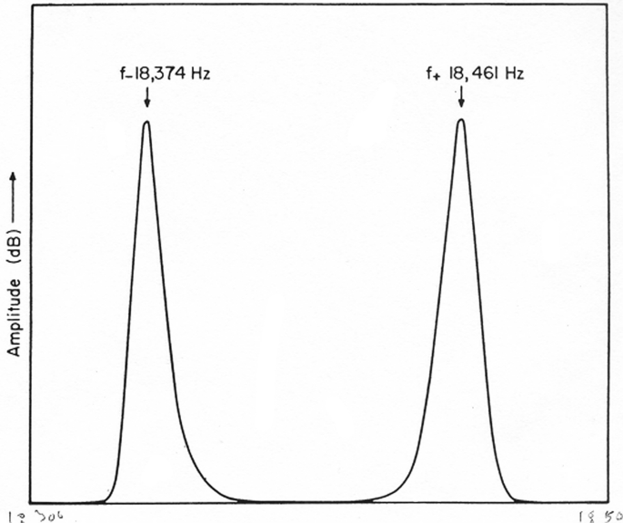

  

  Degenerate modes of a toroidal resonator that are split due to steady flow in the torus

  Fig. 13.26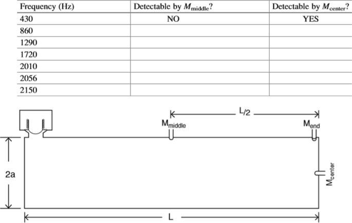

  

  Cross-sectional diagram of a cylindrical resonator that is L long and has a diameter, D = 2a. It is driven by an electrodynamic loudspeaker at the left end of the tube and three microphones are located as shown

Sketched in Fig. 13.27 is the resonance spectrum produced by driving by the loudspeaker and detecting the sound pressure using M_end. The frequency of each peak in the spectrum is labeled.

• (a) Sound speed. If L = 40 cm, what is the speed of sound of the gas contained within the resonator?

• (b) Resonator radius. What is the radius, a (in centimeters), of the resonator?

• (c) Resonance detectability. Complete the table below by indicating which of the resonance peaks would be observable at the middle microphone M_middle and at the microphone at the center of the rigid end M_center by placing a YES in the space if the microphone detects the mode and a NO in the space if that microphone does not detect the mode.

Fig. 13.27

Sketch of the frequency response of the cylindrical resonator shown in Fig. 13.26. The frequency of each resonance is indicated by the arrow, ↓, and is labeled by its frequency in hertz. The signal being displayed was acquired by M_end, located at the intersection of the tube and the end cap opposite the loudspeaker

• 5. Pressure-released rectangular waveguide. The data for phase speed, c_ph vs. frequency, provided in Table 13.9, was obtained for a rectangular, water-filled waveguide, with an anechoic termination, that has a free surface (the air-water interface) and boundaries lined with highly compressible closed-cell foam making all of the boundaries pressure-released. The acoustic pressure in the waveguide was determined by inserting a small hydrophone below the free surface. The hydrophone’s location was determined (±0.5 mm) from a scale attached to the top of the waveguide over distance up to 3 m from the source. The phase speed was determined with an oscilloscope in the x-y (Lissajous) mode, and the distance was recorded to determine the wavelength in the z direction by measuring the distance between successive changes in phase of 360° at precisely known frequencies. Photographs of the waveguide and the anechoic termination are provided in Fig. 13.28.

Table 13.9 Phase speed in a pressure-released waveguide

Fig. 13.28

Waveguide and anechoic termination. (Left) The waveguide is filled with water to a depth of about 17 cm. The three walls of the waveguide are lined with Styrofoam™ to provide a pressure-released surfaces. Note the millimeter scale attached to the top-right edge of the guide. (Right) The anechoic termination, not visible at the left, is shown. It is designed to provide a gently sloping beach of sound absorptive rubber “pyramids”

The phase speed can be expressed in terms of two parameters, the thermodynamic speed of sound in the medium, c_o, and the cut-off frequency, f_co. Transform Eqs. (1.117) or (13.69) so the data in Table 13.9 can be plotted as a straight line and use a best-fit straight line to extract the values for c_o and f_co and their estimated statistical uncertainties.

• 6. Cylindrical waveguide. An air-filled (c = 345 m/sec) semi-infinite rigid tube of circular cross-section (radius, a = 2 cm) is driven at the closed end by a compact source located inside the (closed) end-plane at an intersection of the plane and the tube (z = 0), shown schematically in Fig. 13.29 as the black circle.

  • (a) Number of modes. If the source is driven sinusoidally at a frequency, f = 12.0 kHz, how many propagating modes will be excited and what will be their phase speeds?

  • (b) Excitation of modes. If the source is moved to the center of the end cap, which of the above modes will no longer be excited?

• 7. Group speed. A 20-m-long piece of 6″ (nominal) Schedule 40 PVC pipe (inner radius, a = 5.11 cm) [35] contains air (c = 345 m/s) at atmospheric pressure and is closed at both ends by rigid terminations. A 20.0-millisecond-long tone burst containing 100 cycles of a 5 kHz tone is launched from one of the rigid ends at the intersection of the end and the pipe wall. (See the diagram for Problem 6 in Fig. 13.29.) The pulse propagates to the other end where it is reflected and arrives back at the first end. What is maximum difference in arrival times of the pulse that has been “dispersed” by the fact that the group speed is different for acoustic energy that travels in the different modes? [Hint: The first arrival will be the leading edge of the pulse that made the round trip at the thermodynamic sound speed c_o: t_first = (40 m)/(345 m/s) = 116 ms.]

• 8. Active noise cancellation in an air conditioning duct. Shown in Fig. 13.30 is the block diagram for an active noise control system that injects sound with a loudspeaker that is intended to cancel the sound produced by the “periodic primary source,” for example, a fan that is part of the ventilation system [36]. If the rigid-walled duct has a square cross-section with inside dimension of 1.0 ft. × 1.0 ft., what is the highest-frequency component of the noise that can be cancelled if the control algorithm can only process plane wave fronts traveling at the thermodynamic sound speed in air (c = 345 m/s)?

• 9. Paddle-driven rectangular waveguide. Shown below is the top view of a rigid-walled waveguide that is being driven by a rigid paddle that oscillates sinusoidally at radian frequency, ω = 1400 rad/s, about a fixed axis with an amplitude, θ_o = 0.20 radians, so that θ (t) = 0.20 sin (ωt).

Fig. 13.29

Cylindrical waveguide with a source that is indicated by the solid black circle is located at an intersection of a rigid end cap and the cylindrical waveguide wall

Fig. 13.30

Block diagram of an active noise cancellation system. The duct which contains the loudspeaker and the microphone has a square cross-section that is 1.0 ft × 1.0 ft

The width of the waveguide, W = 40 cm, and the height of the waveguide is much less that its width, H ≪ W. The waveguide extends to infinity in the z direction and is filled with sulfur hexafluoride gas (SF₆) which has a sound speed c = 151 m/s at room temperature (Fig. 13.31).

• (a) Phase Speed. What is the phase speed, c_ph, of the only mode which the paddle is capable of exciting that can propagate down the waveguide in the z direction?

• (b) Group Speed. If the paddle creates a pulse with 17 cycles at the same frequency, ω = 1400 rad/s, by increasing the amplitude of its motion from 0 radians to 0.2 radians and back to 0 radians with the sine-squared amplitude envelope shown in Fig. 13.32, how long does it take for the center of the envelope to travel 100 meters down the waveguide?

• 10. Modes in a non-separable nuclear reactor coolant pool. Shown in Fig. 13.33 is the plan view of a nuclear research reactor cooling pool [37]. It is filed with light (ordinary) water to a depth of 24 ft. = 7.32 m. Other dimensions are included in the caption of Fig. 13.33.

  • (a) Transformed dimensions. What is the equivalent length of the pool, if it is transformed into a uniform rectangular shape that is 4.27 m wide and the depth remains 7.32 m?

  • (b) Lowest-frequency modes. Assuming that the surface of the pool is pressure-released and all the other five boundaries are rigid and impenetrable, determine the 20 lowest-frequency modes and their corresponding mode numbers. Present your results in tabular form.

  • (c) Schroeder frequency and critical distance. The reverberation time measured at 1.6 kHz was T₆₀ = 0.17 s. What are the values of the Schroeder frequency, f_S, and the critical distance, r_d?

  • (d) Number of modes below f_S. Determine the approximate number of modes at frequencies below f_S.

  • (e) Density of modes. What is the density of modes having frequencies below f_S?

• 11. Echo satellite. A gas-filled balloon was launched into low Earth orbit on 12 Aug 1960 to act as a reflector of radio waves used for communications. The balloon, shown symbolically on the postage stamp in Fig. 13.34, had a diameter of 30.5 m, and the balloon’s material was 12.7-micron-thick metalized PET (Mylar™) film [27]. The Echo I satellite re-entered the Earth’s atmosphere and burnt up on 24 May 1968.

Fig. 13.31

This waveguide is excited by the rotational oscillations of the paddle vibrating at angular frequency, ω

Fig. 13.32

Pulse train generated by the oscillating paddle in Fig. 13.31

Fig. 13.33

Plan view of the two coupled pools in the Breazeale Nuclear Reactor. The depth of the water in both bays is 7.32 m (24′). The “floor” of the South Bay is an irregular hemi-hexagon. The reactor’s core is usually located at about the center of that hexagonal portion. For modal calculations, assume that the pool is acoustically equivalent to a rectangular pool with the same planar area. The narrowest portion of the South Bay is 1.22 m wide, and the 14-ft.-wide rectangular portion extends 3.82 m behind the dividing wall. That wall is 46 cm thick and has a 1.52-m-wide gap. Under that adiabatic transformation, the “equivalent” reactor pool should be 4.27 m (14′) wide. Your transformation should preserve the volume of the water contained in both bays. The hemi-hexagonal South Bay has a volume, V_reactor = 151 m³ ≌ 40,000 gallons. The North Bay has a volume, V_storage = 114 m³ ≌ 30,000 gallons. Your modal analysis will designate the vertical direction as the z axis, the width as the x axis (horizontal in this figure), and the length as the y axis (vertical in this figure)

Fig. 13.34

US postage stamp commemorating the Echo Program

• (a) Radial modes. The fundamental frequency of radial mode of the gas inside the balloon was ${f}_{0,0,1}^{\mathrm{release}}$ = 3.6 Hz. What were the frequencies of the next three higher-frequency radial modes?

• (b) Gas sound speed. What was the speed of sound of the gas contained within the balloon?

• 12. Modes of a rigid-walled spherical resonator. Determine the three lowest-frequency radial resonance frequencies for the spherical resonator used by the US National Bureau of Standards, shown in Fig. 13.20, to determine the universal gas constant, ℜ ≡ 8.314462 J mol⁻¹ K⁻¹, if the sphere was filled with argon at T = 273.16 K and standard atmospheric pressure, p_m = 101,325 Pa. The radius of the sphere is a = 9.000 cm.

• 13. Effective radius of the Space Shuttle cargo bay model in Fig. 13.18. Assuming the plastic model of the cargo bay contains air, what is the value of the cargo bay model’s effective radius, a, and its uncertainty, based on the frequencies provided in Table 13.6?

• 14. Waveguide mode excitation. An air-filled waveguide is excited at z = 0 with a transducer that is diagrammed in Fig. 13.35. The waveguide and transducer both have L_x = 15 cm and L_y = 12 cm. The phasing of the nine independent transducer segments is indicated by the + and – signs.

  • (a) Plane wave mode. Will the plane wave mode of the waveguide be excited if the amplitude of all sections are the same?

  • (b) Lowest-frequency non-plane wave modes. What are the mode numbers and cut-off frequencies of the three lowest-frequency non-plane wave modes that will be excited by this transducer?

  • (c) Impulse excitation. If all of the transducer’s segments are excited by a single pulse of very short duration, and the indicated phasing is maintained (e.g., the central segment moves forward and the ones above and below it move backward), which mode will be detected first by a microphone placed a great distance, z ≫ L_x and z ≫ L_y, from the transducer?

Fig. 13.35

Nine-segment transducer that excites a waveguide with the same cross-sectional area

References

L.P. Eisenhart, Separable systems in Euclidean 3-space. Phys. Rev. 45(6), 427–428 (1934)
P.M. Morse, Vibration and Sound, 2nd edn (McGraw-Hill, New York, 1948), p. 396. Reprinted (ASA, 1981). ISBN 0-88318-876-7
B.F.G. Katz, E.A. Wetherill, The fall and rise of the Fogg art Museum lecture hall: A forensic study. Acoust. Today 3(3), 10–16 (2007)
L. L. Beranek, Concert and Opera Halls: How they Sound (Acoustical Society of America, New York, 1996); ISBN 1-56396-530-5
L.L. Beranek, Concert hall acoustics: Recent findings. J. Acoust. Soc. Am. 139(4), 1548–1556 (2016)
J. Liu, S. Garrett, Relationship between Nusselt number and the thermoviscous (Rott) functions. J. Acoust. Soc. Am. 119(3), 1457–1462 (2006). See for discussion of complex compressibility
Sound Absorption and Sound Absorption Coefficients by the Reverberation Room Method, ASTM C423 (American Society for Testing and Materials, Philadelphia, PA 19103)
Measurement of Sound Absorption in a Reverberation Room, ISO 354 (International Organization for Standardization, CH-1211 Geneva 20, Switzerland)
R.J. Peppin, A. Scharine, Methods for Calculation of the Absorption of Sound in the Atmosphere (American National Standard, ANSI/ASA S1.26-2014). See §5.2.1
M.R. Schroeder, The ‘Schroeder frequency’ revisited. J. Acoust. Soc. Am. 99(5), 3240–3241 (1996)
M. Kleiner, J. Tichy, Acoustics of Small Rooms (Taylor & Francis, Boca Raton, 2014); ISBN 978-0-203-86924-6 (eBook-PDF)
K.A. Gillis, M.R. Moldover, A.R.H. Goodwin, Accurate acoustic measurements in gases under difficult conditions. Rev. Sci. Inst. 62, 2213–2217 (1991)
L.D. Landau, E.M. Lifshitz, Fluid Mechanics, 2nd edn. (Butterworth-Heinemann, Oxford, 1987). ISBN 0 7506 2767 0. §15
R. Eisberg, R. Resnick, Quantum Physics of Atoms, Molecules, Solids, Nuclei, and Particles (Wiley, New York, 1974); ISBN 0-471-23464-8
R.T. Weidner, R.L. Sells, Elementary Modern Physics (Allyn and Bacon, Boston, 1960)
L.D. Landau, E.M. Lifshitz, Fluid Mechanics, 2nd edn (Butterworth-Heinemann, Oxford, 1987). See Eq (15.18); ISBN 0 7506 2767 0
M. Abramowitz, I. Stegun, Handbook of Mathematical Functions with Formulas, Graphs, and Mathematical Tables (National Bureau of Standards, Applied Mathematics Series #55, 1964)
E. Polturak, S.L. Garrett, S.G. Lipson, Precision acoustic gas analyzer for binary gas mixtures. Rev. Sci. Inst. 57(11), 2837–2841 (1986)
E. Jahnke, F. Emde, Tables of Functions with Formulae and Curves, 4th edn (Dover, New York, 1945)
P.M. Morse, Vibration and Sound, 2nd edn (McGraw-Hill, 1948). Reprinted by the Acoust. Soc. Am., 1995. See §32; ISBN 0-88318-876-7
I. Rudnick, Physical Acoustics at UCLA in the Study of Superfluid Helium, in Proc. E. Fermi Summer School, Varenna, Italy, 1974
P.M. Morse, K.U. Ingard, Theoretical Acoustics (McGraw-Hill, 1968), Problem 19, pp. 603–604
J.D. Maynard, Topics in Acoustics, Class Notes (The Pennsylvania State University (2006)
D.C. Swanson, Precision spectral peak frequency measurement using a window leakage ratio function. Mech. Systems and Sig. Process 54–55, 1–15 (2015)
M. Greenspan, Simple derivation of the Boltzmann-Ehrenfest adiabatic principle. J. Acoust. Soc. Am. 27(1), 34–35 (1955)
O.B. Wilson, R.W. Leonard, Measurements of sound absorption in aqueous salt solutions using a resonance method. J. Acoust. Soc. Am. 26(2), 223–226 (1954)
H.M. Jones, I.I. Shapiro, P.E. Zadunaisky, Solar radiation effects, gas leakage rates, and air densities inferred from the orbit of Echo I, in Proceedings 2nd International Space Science Symposium, ed. by H.C. Van De Hulst, C. De Jager, A.F. Moore, Florence, April 10–14, 1961 (North Holland, 1961)
P.-J. Shih, Y.-R. Guo, Resonance frequency of fluid-filled and prestressed spherical shell – A model of the human eyeball. J. Acoust. Soc. Am. 139(4), 1784–1792 (2016)
M.R. Moldover, J.P.M. Trusler, T.J. Edwards, J.B Mehl, R.S. Davis, Measurement of the universal gas constant ℜ using a spherical acoustic resonator. Phys. Rev. Lett. 60(4), 249–252 (1988) and M.R. Moldover, et al, J. Res. Natl. Bur. Stand. 93, 85–144 (1988)
L. Pitre, F. Sparasci, L. Risegari, C. Guianvarc’h, C. Martin, M.E. Himbert, M.D. Plimmer, A. Allard, B. Marty, P.A. Giuliano Albo, B. Gao, M.R. Moldover, J.B. Mehl, New measurement of the Boltzmann constant k by acoustic thermometry of helium-4 gas. Metrologia 54, 856–873 (2017)
B.G. Schreger, Laennec’s new system of diagnosis. Q. J. Foreign Med. Surg. 2, 51–68 (1820)
K.U. Ingard, Fundamentals of Waves and Oscillations (Cambridge, 1988); ISBN 0 521 33957 X
C. M. Harris, Noise Control in Buildings: A Practical Guide for Architects and Engineers (McGraw-Hill, 1994); ISBN 0-07-028887-8
C.F. Eyring, Reverberation time in ‘dead’ rooms. J. Acoust. Soc. Am. 1(1), 217–241 (1930)
E.A. Avallone, T. Baumeister II (eds), Marks’ Standard Handbook for Mechanical Engineers, 10th edn (McGraw-Hill, 1996). See Table 8.7.31, pp. 8–193; ISBN 0-07-004997-1
P.A. Nelson, S.J. Elliot, Active Control of Sound (Academic Press, 1993) ISBN 0-12-515426-7
S.L. Garrett, J.A. Smith, R.W.M. Smith, B.J. Heidrich, M.D. Heibel, Using the sound of nuclear energy. Nuc. Technol. 195(3), 353–362 (2016)
Author information
Authors and Affiliations
Rights and permissions
Open Access This chapter is licensed under the terms of the Creative Commons Attribution 4.0 International License (http://creativecommons.org/licenses/by/4.0/), which permits use, sharing, adaptation, distribution and reproduction in any medium or format, as long as you give appropriate credit to the original author(s) and the source, provide a link to the Creative Commons license and indicate if changes were made.
The images or other third party material in this chapter are included in the chapter's Creative Commons license, unless indicated otherwise in a credit line to the material. If material is not included in the chapter's Creative Commons license and your intended use is not permitted by statutory regulation or exceeds the permitted use, you will need to obtain permission directly from the copyright holder.
Copyright information
© 2020 The Author(s)
About this chapter
Cite this chapter
Garrett, S.L. (2020). Three-Dimensional Enclosures. In: Understanding Acoustics. Graduate Texts in Physics. Springer, Cham. https://doi.org/10.1007/978-3-030-44787-8_13
Download citation
DOI: https://doi.org/10.1007/978-3-030-44787-8_13
Published:
Publisher Name: Springer, Cham
Print ISBN: 978-3-030-44786-1
Online ISBN: 978-3-030-44787-8
eBook Packages: Physics and AstronomyPhysics and Astronomy (R0)