Radiation and Scattering

Abstract

At this point, we have made a rather extensive investigation into the sounds that excite Helmholtz resonators as well as the departures from equilibrium that propagate as plane waves through uniform or inhomogeneous media. We have not, as yet, dealt with how those sounds are actually produced in fluids. Our experience tells us that sound can be generated by vibrating objects (e.g., loudspeaker cones, stringed musical instruments, drums, bells), by modulated or unstable flows (e.g., jet engine exhaust, whistles, fog horns, speech), by electrical discharges in the atmosphere (i.e., thunder), or by optical absorption (e.g., modulated laser beams). In this chapter, we will develop the perspective and tools that will be used for the calculation of the radiation efficiency of various sources and combinations of sources, like the sound reinforcement system shown in Fig. 12.1.

At this point, we have made a rather extensive investigation into the sounds that excite Helmholtz resonators as well as the departures from equilibrium that propagate as plane waves through uniform or inhomogeneous media. We have not, as yet, dealt with how those sounds are actually produced in fluids. Our experience tells us that sound can be generated by vibrating objects (e.g., loudspeaker cones, stringed musical instruments, drums, bells), by modulated or unstable flows (e.g., jet engine exhaust, whistles, fog horns, speech), by electrical discharges in the atmosphere (i.e., thunder), or by optical absorption (e.g., modulated laser beams). In this chapter, we will develop the perspective and tools that will be used for the calculation of the radiation efficiency of various sources and combinations of sources, like the sound reinforcement system shown in Fig. 12.1.

Fig. 12.1

Photograph of the sound reinforcement system used by the Grateful Dead [1]. Nearly the entire stage is occupied with discrete vertical line arrays of loudspeakers to radiate the full-frequency spectrum of their music toward the audience with minimal leakage toward the ceiling where there would be excessive reverberation that would degrade the intelligibility

Only sound sources that behave in accordance with linear acoustics will be examined (until Chap. 15). We will find that the entire problem of both radiation and of scattering from small discrete objects can be reduced to understanding the properties of a compact source of sound that is small compared to the wavelength of the sound it is radiating.

“Superposition is the compensation we receive for enduring the limitations of linearity.” Blair Kinsman [2]

We will then combine many of these radiation units, called monopoles, in various ways, including the option of having different units in different locations with different relative phases. Through superposition, this will permit construction of other convenient radiators that range from transversely vibrating incompressible objects (represented by two closely spaced monopoles that are radiating 180° out-of-phase) to arrays of discrete radiators (e.g., line arrays of various sizes like those shown in Fig. 12.1). Integration over infinitesimal monopole sound sources will allow modeling of extended vibrating objects (i.e., continuous, rather than discrete) such as loudspeaker cones, lightning bolts, and laser beams.

For convenience, our initial vision of a compact source will be assumed to be a pulsating sphere with radius, a ≪ λ. That pulsating sphere produces a sinusoidally varying volume velocity, ${U}_1\left(a,t\right)=\mathit{\Re e}\left[\hat{\mathbf{U}}(a){e}^{j\omega\;t}\right]$. To generate such a volume velocity, we will let the radius of that sphere, r, oscillates harmonically with a single frequency, ω = 2πf. Those radial oscillations can be represented as $r(t)=\mathit{\Re e}\left[a+\hat{\boldsymbol{\upxi}}{e}^{j\omega\;t}\right]$; hence $\left|{U}_1\left(a,t\right)\right|=4\uppi {a}^2\omega \left|\hat{\boldsymbol{\upxi}}\right|$, where we have made the assumption that $a\gg \left|\hat{\boldsymbol{\upxi}}\right|$, so that the surface that applies force to the surrounding fluid can be treated as a spherical shell.

As will be demonstrated, an ordinary loudspeaker enclosure, like the one shown in Fig. 12.2, can be treated as a “compact source,” or monopole, if its characteristic physical dimensions are small compared to the wavelength of sound produced. If the loudspeaker enclosures were approximated by a rectangular parallelepiped with volume, V, then “compactness” would require that V^1/3 ≪ λ.

Fig. 12.2

The loudspeaker enclosure at the right has an irregular shape and provides a total enclosed volume, V. To be treated as a “compact source,” we require V^1/3 ≪ λ = c/f = 2πc/ω. The loudspeaker cone, visible at the top of the enclosure, has an effective piston area, A_pist

The oscillatory motion of the loudspeaker cone will be the source of the oscillatory volume velocity in the surrounding fluid. If the cone’s effective piston area is A_pist, located at x = 0, and its linear position as a function of time is ${x}_1\left(0,t\right)=\mathit{\Re e}\left[\hat{\mathbf{x}}{e}^{j\omega\;t}\right]$, then $\left|\hat{\mathbf{U}}\left(0,t\right)\right|=\omega \left|\hat{\mathbf{x}}\right|{A}_{pist}\cos \left(\omega\;t+\phi \right)$.

As long as the compactness criterion is satisfied, it is theoretically impossible to remotely determine the physical shape of a compact source—if the radiation from a source is that of a monopole, then it is only the source’s volume velocity, U₁(a, t), that is related to the sound pressure, p₁(R,t), detected at distances, R ≫ a, beyond the maximum physical extent of the source.¹

Within the constraint of compactness, it does not matter if $\left|\hat{\mathbf{U}}(a)\right|=4\uppi {a}^2\omega \left|\hat{\boldsymbol{\upxi}}\right|$ or $\left|\hat{\mathbf{U}}(0)\right|={A}_{pist}\omega \left|\hat{\mathbf{x}}\right|$, the sound radiated into the far field will be identical. Given that realization, then for a compact source, dimensional analysis guarantees that the solution of the steady-state radiation problem reduces to calculation of the acoustic transfer impedance, ${\mathbf{Z}}_{\mathbf{tr}}=\hat{\mathbf{p}}(R)/\hat{\mathbf{U}}(a)$, with units that are the same as those for the acoustic impedances we have studied in our investigation of lumped elements: |Z_tr| ∝ ρ_mc/A, where ρ_m is the mean density of the medium, c is its sound speed, and A is a constant with the dimensions of area [m²]. The transfer impedances for several systems were provided in Sect. 10.7.4 since they were required to make reciprocity calibrations of electroacoustic transducers.

1 Sound Radiation and the “Causality Sphere”

Light travels at the speed of light; sound travels at the speed of sound. Although those statements seem simplistic, if not tautological, they have calculable consequences that are significant. If a disturbance has a duration, Δt, then those speeds guarantee that the consequences of that event can initially only have influence within a distance, d = cΔt, from the source of that disturbance. The term causality sphere was introduced in Einstein’s Theory of General Relativity as the boundary in spacetime beyond which events cannot affect an outside observer. Although most commonly associated with cosmological issues and black holes, the concept is directly relevant to every form of energy that can only move through space with a finite propagation speed.

Before attempting a direct calculation of the acoustic pressure radiated by a compact source that is pulsating in an unbounded fluid medium, it will be instructive to make a simple estimate of the acoustic transfer impedance between an oscillating source of fluid located at the origin of some coordinate system and the pressure at some remote location, a distance, R, from the origin, using only the adiabatic gas law derived in Sect. 7.1.3: pV ^γ = constant. Before making such a calculation for a source of sound radiating spherically in three dimensions, it will be reassuring to use the same procedure to reproduce a result that we have derived earlier by other means.

If we consider a close-fitting piston at the end of an infinite tube of uniform cross-section,² so that both the tube and the piston have a cross-sectional area, A, then that piston can launch a sound wave down the tube. If the piston produces a volume velocity, $U\left(0,t\right)=\mathit{\Re e}\left[\hat{\mathbf{U}}(0){e}^{j\omega\;t}\right]$, then the acoustic transfer impedance, Z_tr, of such a tube, provided in Eq. (10.85) or in Eq. (10.106), can be used to calculate the steady-state acoustic pressure of the traveling wave produced by the piston’s oscillations.

$$ \hat{\mathbf{p}}={\mathbf{Z}}_{\mathbf{tr}}\hat{\mathbf{U}}(0)=\frac{\rho_mc}{A}\hat{\mathbf{U}}(0)\kern1em \mathrm{and}\kern1em {p}_1\left(x,t\right)=\mathit{\Re e}\left[\hat{\mathbf{p}}{e}^{j\left(\omega\;t- kx\right)}\right] $$

(12.1)

This result describes a plane wave that propagates down the tube with magnitude, $\left|\hat{\mathbf{p}}\right|$, while assuming that thermoviscous dissipation on the tube walls is negligible.

Let’s now calculate this same result in another way. If we consider an interval during which the piston moves between its extreme positions, the piston will sweep out a volume in one-half of a period, $\delta V=\left|\hat{\mathbf{U}}(0)\right|\left(T/2\right)=\left|\hat{\mathbf{U}}(0)\right|/2f$, where T = f⁻¹ = 2π/ω is the period of the piston’s oscillations. In that time, the piston can “influence” a volume of the fluid within the tube, V = (Aλ/2) = (AcT/2), since the sound could travel a distance equal to one-half wavelength. Substitution of δV and V into the adiabatic gas law produces a corresponding δp.

$$ {\displaystyle \begin{array}{c}{pV}^{\gamma } = const.\kern1em \Rightarrow \kern1em \frac{\delta p}{p_m}=-\gamma \frac{\delta V}{V}\kern1em \Rightarrow \kern1em \delta p={p}_1=-\gamma {p}_m\frac{\delta V}{V}\\ {}\left|\hat{\mathbf{p}}\right|=\left|-\gamma {p}_m\frac{T}{2}\frac{\hat{\mathbf{U}}(0)}{Ac\left(T/2\right)}\right|=\frac{\gamma {p}_m\left|\hat{\mathbf{U}}(0)\right|}{Ac}=\frac{\rho_m{c}^2}{Ac}\left|\hat{\mathbf{U}}(0)\right|=\frac{\rho_mc}{A}\left|\hat{\mathbf{U}}(0)\right|\end{array}} $$

(12.2)

The result for $\left|\hat{\mathbf{p}}\right|$ is identical to the previous result from Eq. (12.1).

The situation diagrammed in Fig. 12.3 assumes that there is a compact sphere of radius, a, at the origin of a coordinate system, R = 0. The radius of that sphere oscillates sinusoidally with a radial displacement magnitude, $\left|\hat{\boldsymbol{\upxi}}\right|$. The surface area of that sphere is 4πa², so if $\left|\hat{\boldsymbol{\upxi}}\right|\ll a$, then when the sphere goes from its equilibrium value, a, to its maximum radius, $a+\left|\hat{\boldsymbol{\upxi}}\right|$, it will sweep out a volume change, $\delta V=4\uppi {a}^2\left|\hat{\boldsymbol{\upxi}}\right|$. The time it takes to sweep that volume change is one-quarter of the acoustic period, T/4 = (4f)⁻¹.

Fig. 12.3

The “Sphere of Causality.” This diagram represents two concentric spheres. The inner sphere has a radius, a. That radius oscillates sinusoidally at a frequency, f = ω/2π, with an amplitude, $\left|\hat{\boldsymbol{\upxi}}\right|$. The radius of the inner sphere goes from its equilibrium value, r = a, to its maximum displacement, $r=a+\left|\hat{\boldsymbol{\upxi}}\right|$, in one-quarter of an acoustic period: T/4 = (4f)⁻¹. During that time, the effects of that displacement of fluid volume, $\delta V=4\uppi {a}^2\left|\hat{\boldsymbol{\upxi}}\right|$, can only propagate a distance of one-quarter wavelength from the origin, R_λ/4 = λ/4 = c/4f. That distance is the radius of the causality sphere since information carried by sound can only propagate at the speed of sound, c. The volume enclosed by that “causality sphere,” indicated by the dashed circle in two dimensions, is V_λ/4 = (π/48)λ³

Since the speed of sound is c, any “disturbance” created by the source during that quarter period can only influence the fluid out to a distance, R_λ/4 = c(T/4) from the source. Let’s assume we are making a video that starts when the spherical source goes through its equilibrium radius, r = a, then continues expanding for one-quarter of an acoustic period, T/4. During that time interval, the source changes its volume by δV = U₁(a)/ω, since the radius is changing sinusoidally with time, pushing fluid out ahead of it. Once again, as in Eq. (12.2), logarithmic differentiation of the adiabatic gas law will relate the average pressure change, <p₁(R)>_s, within the causality sphere of volume, V_λ/4 = (4π/3)R³ = (π/48)λ³, to δV.

$$ \frac{{\left\langle {p}_1\right\rangle}_s}{p_m}=\gamma \frac{\delta V}{V_{\lambda /4}}\kern1em \Rightarrow {\left\langle {p}_1\right\rangle}_s=\gamma {p}_m\frac{\left|\hat{\mathbf{U}}(a)\right|}{\omega\;{V}_{\lambda /4}}={\rho}_m{c}^2\frac{\left|\hat{\mathbf{U}}(a)\right|}{\omega\;{V}_{\lambda /4}} $$

(12.3)

The final version at the right of Eq. (12.3) again uses the fact that the square of the sound speed in an ideal gas is given by c² = γp_m/ρ_m. We can solve for the average acoustic transfer impedance <Z_tr>_s = <p₁(R)/U₁(a)>_s between the volume velocity at the surface of the source, U₁(a), and the average pressure, <p₁(R)>_s, at an observation point just inside the causality sphere at R = λ/4.

$$ {\left\langle {\mathbf{Z}}_{\mathbf{tr}}\right\rangle}_s=\frac{{\left\langle {p}_1(R)\right\rangle}_s}{U_1(a)}=\frac{6}{\uppi^2}\frac{\rho_mc}{R\lambda}\cong 0.61\frac{\rho_mc}{R\lambda} $$

(12.4)

As we will see when we solve the exact hydrodynamic equations, this approximate result is close to the exact result, which produces a numerical pre-factor for Eq. (12.4) that is 0.50 instead of 0.61.

This result is only approximate since the actual acoustic pressure within the “causality sphere” is a function of the distance from the source. We would have obtained a different result for the numerical pre-factor in Eq. (12.4) had we let the “event” last one-half period so that the source went from its minimum radius, $a-\left|\hat{\boldsymbol{\upxi}}\right|$, to its maximum radius, $a+\left|\hat{\boldsymbol{\upxi}}\right|$. That change in volume, δV, would be doubled, but the volume of the “causality sphere” would have increased by a factor of eight. Under that scenario, the numerical pre-factor in Eq. (12.4) would have decreased from 0.61 to 0.15.

This variability is due to the fact that the pressure within the causality sphere is not uniform. We expect wavelike motion, not simple hydrostatic compression, as assumed by the use of the adiabatic gas law in Eq. (12.2) to produce δp. This was not an issue in the causality calculation for the duct where p₁ was uniform throughout for a traveling wave in one dimension, since the “average” and the amplitude were identical. For the three-dimensional case, acoustic pressure amplitude is a function of distance from the source.

The purpose of such a crude calculation was to demonstrate that the earlier concepts introduced to produce an equation of state, describe sound in lumped-element networks, or for one-dimensional propagation are just as relevant to understanding the process of sound radiation. In the next section, the exact result will be derived when the wave equation is solved exactly for a spherically symmetric wave expanding in three dimensions.

2 Spherically Diverging Sound Waves

The exact result for the acoustic transfer impedance, Z_tr, which provides the acoustic pressure at every remote location, p₁(R), in terms of the volume velocity created at the source, U₁(a), can be obtained if we solve the wave equation in spherical coordinates. The Euler equation, also expressed in spherical coordinates, can be used to match the radial velocity of the fluid to the radial velocity of the compact spherical source, ${\hat{\mathbf{v}}}_{\mathbf{r}}(a)$, remembering that the representation of the volume velocity of the source as a pulsating sphere is only a mathematical convenience. The result will be applicable to any compact source, independent of its shape.

When the wave equation was derived in Cartesian coordinates in Sect. 10.2, the result was generalized by expressing the wave equation in vector form by introducing the Laplacian operator, ∇² = ∂²/∂x² + ∂²/∂y² + ∂²/∂z². For the compact source in an unbounded medium, a spherical coordinate system would be appropriate (and convenient) since all directions are equivalent; we expect no variation in the sound field with either polar angle, 90° ≥ θ ≥ −90°, or azimuthal angle 0° ≤ φ < 360°. In spherical coordinates, the Laplacian can be written in terms of r, θ, and φ [3].

$$ {\nabla}^2=\frac{1}{r^2}\left[\frac{\partial }{\partial r}\left({r}^2\frac{\partial }{\partial r}\right)\right]+\frac{1}{r^2\sin \theta}\frac{\partial }{\partial \theta}\left(\sin \theta \frac{\partial }{\partial \theta}\right)+\frac{1}{r^2{\sin}^2\theta}\frac{\partial^2}{\partial {\varphi}^2} $$

(12.5)

Since the space surrounding our source is assumed to be isotropic, hence spherically symmetric, p₁(R) does not depend upon θ or φ, so derivatives with respect to those variables must vanish. Equation (12.5) can be substituted into the linearized wave equation.

$$ {\nabla}^2p=\frac{1}{r^2}\left[\frac{\partial }{\partial r}\left({r}^2\frac{\partial p}{\partial r}\right)\right]=\frac{1}{c^2}\frac{\partial^2p}{\partial {t}^2} $$

(12.6)

The “product rule” for differentiation can be used to demonstrate that Eq. (12.6) is equivalent to Eq. (12.7).

$$ \frac{\partial^2(rp)}{\partial {r}^2}=\frac{1}{c^2}\frac{\partial^2(rp)}{\partial {t}^2} $$

(12.7)

This is just a new single parameter (i.e., quasi-one-dimensional) wave equation that describes the space and time evolution of the product of radial distance from the origin and the acoustic pressure at that distance, (rp); hence the solution to Eq. (12.7) is $(pr)=\mathit{\Re e}\left[\hat{\mathbf{C}}{e}^{j\left(\omega\;t\mp kr\right)}\right]$, where $\hat{\mathbf{C}}$ is a constant (phasor) that may be complex to account for any required phase shift and an arbitrary designation of the time we chose to make t = 0. We will specify that complex (phasor) amplitude, $\hat{\mathbf{C}}$, by matching this solution to the volume velocity of the source at its surface, r = a. The two solutions to Eq. (12.7) correspond to outgoing (ωt – kr) or incoming (ωt + kr) spherical waves, also referred to as divergent and convergent waves, respectively. Since we are considering radiation from a sound source in a homogeneous, isotropic, unbounded medium (i.e., no reflections), we will now focus only on the outgoing solution.

$$ {p}_1\left(r,t\right)=\mathit{\Re e}\left[\frac{\hat{\mathbf{C}}}{r}{e}^{j\left(\omega\;t- kr\right)}\right] $$

(12.8)

The magnitude of the acoustic pressure decreases with distance from the source. As will be demonstrated in the derivation of Eq. (12.18), the total radiated power, Π_rad, is independent of distance from the source’s acoustic center (i.e., the origin of our spherical coordinate system) if dissipation is ignored.

To match the velocity of the fluid to the velocity of the source at its surface, r = a, Eq. (12.8) can be substituted into the linearized Euler equation.

$$ {\rho}_m\frac{\partial \overrightarrow{v}}{\partial t}=-\overrightarrow{\nabla}p $$

(12.9)

The gradient operator, $\overrightarrow{\nabla}$, can also be expressed in spherical coordinates [3].

$$ \overrightarrow{\nabla}p\left(r,\theta, \varphi \right)=\frac{\partial p\left(r,\theta, \varphi \right)}{\partial r}\hat{r}+\frac{1}{r}\frac{\partial p\left(r,\theta, \varphi \right)}{\partial \theta}\hat{\theta}+\frac{1}{r\sin \theta}\frac{\partial p\left(r,\theta, \varphi \right)}{\partial \varphi}\hat{\varphi} $$

(12.10)

Again, for our spherically symmetric case, p₁(r, t) is independent of θ and φ, so only the first term on the right-hand side of Eq. (12.10) is required to calculate the radial component of the wave velocity, v_r (r, t). The application of the product rule generates two terms.

$$ {\displaystyle \begin{array}{c}{\rho}_m\frac{\partial {v}_r}{\partial t}=-\frac{\partial }{\partial r}\left[\frac{\hat{\mathbf{C}}}{r}{e}^{j\left(\omega \kern0.1em t- kr\right)}\right]\\ {}=\frac{\hat{\mathbf{C}}}{r^2}{e}^{j\left(\omega\;t- kr\right)}+ jk\frac{\hat{\mathbf{C}}}{r}{e}^{j\left(\omega\;t- kr\right)}=\frac{\hat{\mathbf{C}}}{r}{e}^{j\left(\omega \kern0.1em t- kr\right)}\left[\frac{1}{r}+ jk\right]\end{array}} $$

(12.11)

Since we have assumed single-frequency harmonic time dependence, the time derivative in Eq. (12.11) can be replaced by jω while recalling that c = ω/k.

$$ {v}_r\left(r,t\right)=\mathit{\Re e}\left[\frac{p_1\left(r,t\right)}{j{\omega \rho}_m}\left(\frac{1}{r}+ jk\right)\right]=\mathit{\Re e}\left[\frac{p_1\left(r,t\right)}{\rho_mc}\left(1+\frac{1}{jkr}\right)\right] $$

(12.12)

2.1 Compact Monopole Radiation Impedance

Equation (12.12) can be rewritten to provide the specific acoustic impedance, ${\mathbf{z}}_{\mathbf{sp}}=\hat{\mathbf{p}}/{\hat{\mathbf{v}}}_{\mathbf{r}}$, for propagation of outgoing (diverging) spherical waves. As with plane waves, the sign of the specific acoustic impedance is reversed for incoming (convergent) spherical waves.

$$ {\mathbf{z}}_{\mathbf{sp}}\equiv \frac{\hat{\mathbf{p}}}{{\hat{\mathbf{v}}}_{\mathbf{r}}}=\frac{\rho_mc}{1+\left(\raisebox{1ex}{$1$}\!\left/ \!\raisebox{-1ex}{$ jkr$}\right.\right)}={\rho}_mc\frac{(kr)^2}{1+{(kr)}^2}+j{\rho}_mc\frac{kr}{1+{(kr)}^2}={\rho}_mc\cos \phi\;{e}^{j\phi} $$

(12.13)

All three versions of Eq. (12.13) are useful, although in different contexts. The rightmost version suggests a geometric interpretation based on Fig. 12.4.

Fig. 12.4

Geometric interpretation of Eq. (12.13) representing the phase, ϕ, of the (complex) specific acoustic impedance, z_sp, for an outgoing spherical wave. The phase angle, ϕ, between the acoustic pressure, $\hat{\mathbf{p}}$, and the radial component of the acoustic particle velocity, ${\hat{\mathbf{v}}}_{\mathbf{r}}$, is ϕ = cot⁻¹(kr)

For very large values of kr, the curvature of the spherical wave fronts is slight, and the wave fronts (locally) are approximately planar. For kr = 2πr/λ ≫ 1, ${\mathbf{z}}_{\mathbf{sp}}=\hat{\mathbf{p}}/{\hat{\mathbf{v}}}_{\mathbf{r}}\cong {\rho}_mc$, for the propagation of outgoing (diverging) spherical waves, as shown by the solid line in Figs. 12.5 and 12.6 that approaches that constant value as ka increases. The specific acoustic impedance becomes a real number, and the acoustic pressure, $\hat{\mathbf{p}}$, and the radial component of the fluid’s acoustic particle velocity, ${\hat{\mathbf{v}}}_{\mathbf{r}}$, are very nearly in-phase, ϕ ≌ 0°.

Fig. 12.5

The complex radiation impedance of a monopolar sound source, z_sp, divided by the fluid medium’s characteristic impedance, ρ_mc, from Eq. (12.13). The solid line is the real part of the radiation impedance, and the dashed line is the imaginary part. For small ka, the slope of the imaginary part is initially proportional to frequency, indicating mass-like behavior of the fluid at the monopole’s surface

Fig. 12.6

The complex radiation impedance of a monopolar sound source, z_sp, divided by the fluid medium’s characteristic impedance, ρ_mc, from Eq. (12.13), except that the horizontal axis is now logarithmic. The solid line is the real part of the radiation impedance, and the dashed line is the imaginary part. Plotted this way, the similarity to Fig. 4.25 and Fig. 5.20, for the real and imaginary elastic modulus of a viscoelastic solid, and Fig. 14.3 or Fig. 14.4, for the sound speed and attenuation in F₂, is apparent

It is instructive to reproduce Fig. 12.5, but with a logarithmic ka axis as shown in Fig. 12.6. The similarity between the shape of the real and imaginary portions of the radiation impedance and the real and imaginary parts of the elastic modulus in Fig. 4.25 and Fig. 5.20, or the sound speed and attenuation in fluorine gas in Fig. 14.4, is not coincidental. It is a consequence of any linear response theory that is constrained by causality, as specified in the Kramers-Kronig relations of Eqs. (4.77) and (4.78), discussed in Sect. 4.4.4. Just as in those examples, the real and imaginary parts of the radiation impedance are not independent [4].

In the opposite limit, at ka = 2πa/λ ≪ 1,³ on the surface of the radially pulsating source, the specific acoustic impedance is almost purely imaginary, as shown by the dashed line in Figs. 12.5 and 12.6.

$$ \underset{ka\to 0}{\lim}\left[{\mathbf{z}}_{\mathbf{sp}}(a)\right]\cong j{\rho}_m cka= j\omega\;{\rho}_ma $$

(12.14)

Recalling our experience with the simple harmonic oscillator, Eq. (12.14) suggests that the fluid surrounding the source is behaving like an effective mass. The magnitude of the force, $\left|\hat{\mathbf{F}}(a)\right|$, acting on the pulsating sphere can be obtained by integrating the pressure, $\hat{\mathbf{p}}(a)$, over the surface of the sphere to produce the mechanical reactance, x_rad(a) = ℑm[Z_mech(a)], that the pulsating sphere “feels” at its surface.

$$ {\displaystyle \begin{array}{c}\mathit{\Im m}\left[{\mathbf{Z}}_{\mathbf{mech}}\right]=\kern0.15pc \mathit{\Im m}\left[\frac{\hat{\mathbf{F}}(a)}{{\hat{\mathbf{v}}}_{\mathbf{r}}(a)}\right]=4\uppi {a}^2\left({\rho}_m\omega\;a\right)\\ {}=\kern0.15pc {\omega \rho}_m\left(4\uppi {a}^3\right)=3{\omega \rho}_m\left(\frac{4\uppi}{3}{a}^3\right)\kern1em \mathrm{for}\kern1em ka\ll 1\end{array}} $$

(12.15)

The volume of the spherical source is V = (4π/3)a³, so the effective (inertial) hydrodynamic mass of the fluid surrounding the spherical source is equal to three times the mass of the fluid displaced by the source radiating sound in the small ka limit.

This is critical for the design of sound sources that operate in dense fluids (i.e., liquids rather than gases) since the source has to provide sufficient power to accelerate and decelerate the surrounding fluid as it pulsates. We generally represent this load as a radiation reactance, x_rad. As will be discussed shortly, in Sect. 12.3, for a spherical gas bubble in a liquid, this effective mass is the dominant source of inertia for simple harmonic bubble oscillations.

Although the largest component of the specific acoustic impedance at the surface of the sphere is imaginary (i.e., mass reactance), the real (i.e., resistive) component must be non-zero, because radiation of sound is the mechanism by which energy from the source is propagated into the surrounding fluid. The second version of z_sp in Eq. (12.13) is useful here since it provides the real and imaginary contributions individually.

$$ \mathit{\Re e}\left\{\underset{ka\to 0}{\lim}\left[{\mathbf{z}}_{\mathbf{sp}}(a)\right]\right\}\equiv {r}_{rad}\cong {\rho}_mc{(ka)}^2 $$

(12.16)

It is worthwhile pointing out that real impedances are commonly associated with dissipative processes that convert acoustical or vibrational energy to heat. In the case of radiation, power is removed from the source, but our calculations have been lossless (i.e., we have been using the Euler equation, not the Navier-Stokes equation). The real component of the radiation impedance is an “accounting loss” rather than an irreversible increase in entropy. For radiation, the energy propagates away; it is not absorbed, its expelled.

The total, time-averaged radiated acoustic power, 〈Π_rad〉_t, is the rate at which the source does “p∗dV” work on the surrounding fluid for the in-phase components of the acoustic pressure, $\hat{\mathbf{p}}(a)$, and the (radial) acoustic particle velocity, ${\hat{\mathbf{v}}}_{\mathbf{r}}(a)$, at the source’s surface.

$$ {\displaystyle \begin{array}{c}{\left\langle {\Pi}_{rad}\right\rangle}_t=\frac{1}{T}{\int}_0^T\hat{\mathbf{F}}(a)\cdotp {\hat{\mathbf{v}}}_{\mathbf{r}}(a)\;\mathrm{d}t\;\mathrm{d}S=\frac{1}{T}{\int}_0^T\left|\hat{\mathbf{p}}(a)\right|\;\left|\frac{\mathrm{d}V(a)}{\mathrm{d}t}\right|\cos \phi\;\mathrm{d}t\\ {}=\frac{1}{T}{\int}_0^T\left|\hat{\mathbf{p}}(a)\right|\;\left|\hat{\mathbf{U}}(a)\right|\cos \phi\;\mathrm{d}t\end{array}} $$

(12.17)

The component of $\hat{\mathbf{p}}(a)$ that is in-phase with ${\hat{\mathbf{v}}}_{\mathbf{r}}(a)$ can be expressed in terms of the radiation resistance, r_rad, which is the real part of the specific acoustic impedance, z_sp(a), on the surface of the sphere. Since $\mathit{\Re e}\left[\hat{\mathbf{p}}(a)\right]={r}_{rad}\left|{\hat{\mathbf{v}}}_{\mathbf{r}}(a)\right|$ and $\left|\hat{\mathbf{U}}(a)\right|=4\uppi {a}^2\left|{\hat{\mathbf{v}}}_{\mathbf{r}}(a)\right|$, we can express Eq. (12.17) in terms of r_rad and ${\hat{\mathbf{v}}}_{\mathbf{r}}(a)$.

Using the expression for r_rad in Eq. (12.16) and expressing ${\hat{\mathbf{v}}}_{\mathbf{r}}(a)$ in terms of the magnitude of the source strength, $\left|\hat{\mathbf{U}}(a)\right|$, provide a compact expression for the time-averaged power, 〈Π_rad〉_t, radiated from the source based on the real component of the specific acoustic impedance at the source’s surface, ℜe[z_sp(a)] ≡ r_rad.

$$ {\left\langle {\Pi}_{rad}\right\rangle}_t=\frac{\uppi}{2}\frac{\rho_mc}{\lambda^2}{\left|\hat{\mathbf{U}}(a)\right|}^2=\frac{\uppi}{2}\frac{\rho_m}{c}{f}^2{\left|\hat{\mathbf{U}}(a)\right|}^2 $$

(12.18)

The right-hand version of this result demonstrates why it is more difficult to radiate low frequencies. Either the velocity of the surface needs to be increased, which frequently causes distortion, or the loudspeaker’s area must be increased, assuming that (ka)² ≪ 1. This is why the enclosures for reproduction of bass utilize loudspeakers of large diameter to provide adequate source strength, $\left|\hat{\mathbf{U}}(a)\right|$, as suggested in Fig. 12.1.

2.2 Compact Monopole Acoustic Transfer Impedance

To determine the amplitude constant, $\hat{\mathbf{C}}$, in Eq. (12.8), we can consider our pulsating sphere of mean radius, a, and radial velocity, ${\hat{\mathbf{v}}}_{\mathbf{r}}(a)= j\omega\;\hat{\boldsymbol{\upxi}}$, and evaluate Eq. (12.12) at r = a.

$$ {v}_r\left(a,t\right)=\mathit{\Re e}\left[ j\omega\;\hat{\boldsymbol{\upxi}}\;{e}^{j\omega\;t}\right]=\mathit{\Re e}\left[\frac{\hat{\mathbf{C}}}{a{\rho}_mc}{e}^{j\left(\omega\;t- ka\right)}\left(1+\frac{1}{j ka}\right)\right] $$

(12.19)

The compactness requirement guarantees that ka ≪ 1, so e^−jka ≅ 1 and [1 + (1/jka)] ≌ (1/jka). Substituting these near-field limits into Eq. (12.19), along with the fact that $\left|\hat{\mathbf{U}}(a)\right|=4\uppi {a}^2\left|{\hat{\mathbf{v}}}_{\mathbf{r}}(a)\right|$, uniquely determines the complex (phasor) pressure amplitude constant, $\hat{\mathbf{C}}$.

$$ \hat{\mathbf{C}}=\omega \kern0.1em {\rho}_mc\;\hat{\boldsymbol{\upxi}}\;{ka}^2=\frac{\rho_m ck}{4\uppi}\hat{\mathbf{U}}(a) $$

(12.20)

Substitution of $\hat{\mathbf{C}}$ back into Eq. (12.8) provides the exact solution for the acoustic pressure, p₁(r,t), in terms of the magnitude of the source’s volume velocity, $\left|\hat{\mathbf{U}}(a)\right|$, and the wavelength of sound, λ = (2π/k).

$$ {p}_1\left(r,t\right)=\frac{\rho_m ck}{4\pi r}\left|\hat{\mathbf{U}}(a)\right|\mathit{\Re e}\left[{e}^{j\left(\omega\;t- kr\right)}\right]=\frac{\rho_mc}{2 r\lambda}\left|\hat{\mathbf{U}}(a)\right|\mathit{\Re e}\left[{e}^{j\left(\omega\;t- kr\right)}\right] $$

(12.21)

The exact solution for the acoustic transfer impedance, Z_tr, can be calculated from Eq. (12.21), providing the solution to this steady-state radiation problem.

$$ \left|{\mathbf{Z}}_{\mathbf{tr}}\right|\equiv \left|\frac{\hat{\mathbf{p}}(R)}{\hat{\mathbf{U}}(a)}\right|=\frac{\rho_mc}{2 R\lambda}=0.50\frac{\rho_mc}{R\lambda} $$

(12.22)

This result compares closely to the “causality sphere” approximation of Eq. (12.4) that was based on the adiabatic gas law but ignored the wavelike variation in pressure with position that is expressed exactly in Eq. (12.8).

The acoustic transfer impedance will now let us express the acoustic pressure, $\hat{\mathbf{p}}(R)$, at some remote point in the far field (kR ≫ 1), a distance, R, from the sound source’s acoustic center, R = 0. This compact sound source of source strength, |U₁(a)|, radiates sound with a wavelength, λ = c/f = 2πc/ω. At that location in the far field, we can assume that $\hat{\mathbf{p}}(R)$ is in-phase with ${\hat{\mathbf{v}}}_{\mathbf{r}}(R)$, based on Eq. (12.13), and that their ratio is given by the progressive plane wave value of the characteristic impedance z_sp (R) = ρ_mc. This simplifies the calculation of the far-field time-averaged intensity of the sound, ${\left\langle \overrightarrow{I}(R)\right\rangle}_t$, using Eq. (10.36).

$$ {\displaystyle \begin{array}{c}{\left\langle \overrightarrow{I}(R)\right\rangle}_t=\kern0.15pc \left(\frac{1}{2}\right)\mathit{\Re e}\left[\hat{\mathbf{p}}(R){\hat{\mathbf{v}}}_{\mathbf{r}}^{\ast}(R)\right]=\frac{{\left|\hat{\mathbf{p}}(R)\right|}^2}{2{\rho}_mc}\\ {}=\frac{1}{2{\rho}_mc}{\left(\frac{\rho_mc}{2 R\lambda}\left|\hat{\mathbf{U}}(a)\right|\right)}^2=\frac{\rho_mc}{8{R}^2{\lambda}^2}{\left|\hat{\mathbf{U}}(a)\right|}^2\end{array}} $$

(12.23)

The time-averaged acoustic intensity is inversely proportional to the square of the distance from the sound source, but the time-averaged total radiated power, 〈Π_rad〉_t, is independent of distance, since all forms of dissipation have been neglected.

$$ {\left\langle {\Pi}_{rad}\right\rangle}_t=4\uppi {R}^2{\left\langle I(R)\right\rangle}_t=\frac{\uppi}{2}\frac{\rho_mc}{\lambda^2}{\left|\hat{\mathbf{U}}(a)\right|}^2 $$

(12.24)

Of course, in the absence of any dissipation in the surrounding fluid, this is the same radiated power we calculated “locally” by using the radiation resistance “felt” by the source, r_rad (a), on its surface (i.e., in the near field), expressed in Eq. (12.18).

2.3 General Multipole Expansion*

Since the monopole is such a significant concept for our understanding of radiation and scattering, it is worthwhile to review the assumptions and processes that led to the results of Eqs. (12.13), (12.15), (12.18), (12.19), (12.21), (12.22), and (12.23). Fundamentally, the three-dimensional problem of Eq. (12.5) was transformed to the quasi-one-dimensional problem of Eq. (12.6) based on a claim of spherical symmetry (i.e., isotropy) and the assertion that the shape of the pulsating source of volume velocity was irrelevant (and unknowable based on the far-field radiation pattern),¹ so that only the source strength, $\left|\hat{\mathbf{U}}(a)\right|$, was significant for determination of the radiated sound field.

That assertion of source-shape independence was not proven, since it would be necessary to solve the full three-dimensional problem, then determine under what circumstances the higher-order multipolar contributions are negligible. The solution to the full three-dimensional problem, using the Laplacian of Eq. (12.5) in the wave equation, is a product of spherical Bessel functions, j_n (kr), and the associated Legendre polynomials, ${P}_l^m\left(\cos\;\theta \right)$.

$$ p\left(r,\theta, \vartheta; t\right)=\mathit{\Re e}\left[\sum {\hat{\mathbf{C}}}_{\mathbf{n},\mathbf{m},\mathbf{l}}{e}^{j\omega\;t}{j}_n(kr)\sqrt{\frac{2l+1}{2\uppi}\frac{\left(l-m\right)!}{\left(l+m\right)!}}{P}_l^m\left(\cos \theta \right)\left\{\begin{array}{c}\cos \left( m\varphi \right)\\ {}\sin \left( m\varphi \right)\end{array}\right\}\right] $$

(12.25)

The constants, ${\hat{\mathbf{C}}}_{\mathbf{n},\mathbf{m},\mathbf{l}}$, are determined in the same way as we determined $\hat{\mathbf{C}}$ in Eq. (12.8); by matching the velocity components of the wave (using Euler’s equation) to the velocity distribution on the surface of the source. The complete set of functions provided in the infinite summation of Eq. (12.25) can be fit to a source of any shape where the various parts of the surface are moving in any direction and with any relative phase, although the result is still restricted to a single frequency [5]. Our solution of Eq. (12.8) corresponds to the spherically symmetric n = 0 spherical Bessel function, j₀ (kr) = sin (kr)/(kr), which forces m = l = 0, so that there is no angular dependence.⁴

Our analysis, based on a compact spherical source, produced results that are applicable to sound sources that have no resemblance to a sphere, for example, a circular piston executing simple harmonic oscillations mounted in an enclosure that is a rectangular parallelepiped or the body of a dog (e.g., Fig. 12.2). The results obtained only depend upon specification of the source strength, $\left|\hat{\mathbf{U}}(a)\right|$, and our ability to enclose the source within a spherical shell having a circumference much less than the wavelength (i.e., ka ≪ 1) that is pulsating with a complex radial oscillation amplitude, $\hat{\boldsymbol{\upxi}}$, making the source strength magnitude, $\left|\hat{\mathbf{U}}(a)\right|=4\uppi {a}^2\omega \left|\hat{\boldsymbol{\upxi}}\right|$.

After using hydrodynamic mass to calculate the resonance frequency of a bubble in the next section, we will continue to avoid dealing with the complete mathematical solution of Eq. (12.25) by using the principle of superposition to sum the acoustic fields of simple monopole sources. This will facilitate calculation of the behavior of more complex sources that lack spherical symmetry and produce a significant angular dependence of their radiated sound fields.

3 Bubble Resonance

Having calculated the hydrodynamic mass associated with the radial oscillations of a compact spherical source in Eq. (12.15), this concept can be applied to an interesting and important lumped-element fluidic resonator for which the hydrodynamic mass makes the entire inertial contribution. A gas bubble in a liquid will have an equilibrium radius, a, that is determined by the competition between the surface tension that will cause the bubble to collapse and the gas pressure inside the bubble that will resist the external force of the liquid pressure and of the surface tension.

The static pressure difference, p_in – p_out, across a curved interface is given by Laplace’s formula that can be expressed in terms of the principle radii of curvature and the surface tension, α [6].

$$ {p}_{in}-{p}_{out}=\alpha \left(\frac{1}{R_1}+\frac{1}{R_2}\right) $$

(12.26)

For a spherical bubble, R₁ = R₂ = a, where a is the radius of the bubble, so the pressure difference caused by the surface tension is 2α/a. If the gas inside the bubble is the vapor of the surrounding liquid, then there will be a minimum bubble radius, R_min, determined when the vapor pressure and Laplace pressures are equal. In the case where a < R_min, the bubble is unstable and will collapse by squeezing the vapor back into the liquid state.

For a “clean” air-water interface at 20 °C, the surface tension, α = 72.5 × 10⁻³ N/m, and P_vap = 2.3 kPa, so R_min = 0.063 mm = 63 μm. As we will see, our interests are concentrated on larger bubbles, many of which may contain a non-condensable gas (e.g., air) that stabilizes the bubbles against collapse.

The gas pressure, p_in, within a stable bubble surrounded by water, is usually determined by the depth of the bubble below the water’s surface. Since p_in = p_o + ρ_mg z, where p_o is atmospheric pressure, g is the acceleration due to gravity, ρ_m is the mass density of the water (not the gas!), and z is the distance below the free surface, as discussed in Sect. 8.3. If the mean radius of the bubble, a, is displaced from equilibrium by an amount, $\left|\hat{\boldsymbol{\upxi}}\right|$, while maintaining its spherical shape, the excess force, $\delta F\left(\hat{\boldsymbol{\upxi}}\right)$, that the pressure applies to the bubble’s surface can be determined from the adiabatic gas law, if we assume that a > δ_κ, so the compressions and expansions are nearly adiabatic, again using Eq. (12.2).

$$ \delta {p}_{in}=-\gamma {p}_{in}\frac{\delta V}{V}=-\gamma {p}_{in}\frac{4\uppi {a}^2\left|\hat{\boldsymbol{\upxi}}\right|}{\left(\raisebox{1ex}{$4\uppi $}\!\left/ \!\raisebox{-1ex}{$3$}\right.\right){a}^3}=-3\gamma {p}_{in}\frac{\left|\hat{\boldsymbol{\upxi}}\right|}{a} $$

(12.27)

Integrated over the surface area of the bubble, this excess pressure, $\delta {p}_{in}=\left|\hat{\mathbf{p}}\right|$, produces an excess force, $\delta F\left(\hat{\boldsymbol{\upxi}}\right)$, which is proportional to the amplitude of the oscillatory change in radius, $\hat{\boldsymbol{\upxi}}$, and motivates an expression that is equivalent to Hooke’s law:

$$ \delta F=\left(4\uppi {a}^2\right)\delta {p}_{in}=-12\uppi a\gamma {p}_{in}\left|\hat{\boldsymbol{\upxi}}\right|\kern1em \Rightarrow \kern1em {\mathrm{K}}_{eff}=12\uppi a\gamma {p}_{in} $$

(12.28)

The minus signs in Eqs. (12.27) and (12.28) arise because the pressure increases when $\left|\hat{\boldsymbol{\upxi}}\right|$ decreases. By analogy with Hooke’s law, the effective stiffness constant, Κ_eff, is just the magnitude of the coefficient of such displacements, $\hat{\boldsymbol{\upxi}}$.

The only inertial mass of any significance is the hydrodynamic mass, m_eff, of the fluid that must accelerated in and out radially as the bubble’s radius changes. This hydrodynamic mass can be calculated using Eq. (12.15).

$$ {m}_{eff}=3{\rho}_mV=4\uppi {a}^3{\rho}_m $$

(12.29)

That effective mass can be combined with the effective gas stiffness of Eq. (12.28) to create a simple harmonic oscillator with a resonance frequency, f_o = ω_o/2π.

$$ {\omega}_o=\sqrt{\frac{{\mathrm{K}}_{eff}}{m_{eff}}}=\frac{1}{a}\sqrt{\frac{3\gamma {p}_{in}}{\rho_m}} $$

(12.30)

Here, it is important to remind ourselves that p_in is the gas pressure but ρ_m is the density of the surrounding water. If the restoring force due to surface tension is included, Eq. (12.30) can be modified to incorporate that additional restoring force (stiffness) [7].

$$ {\omega}_o=\frac{1}{a\sqrt{\rho_m}}\sqrt{3\gamma {p}_{in}-\frac{2\alpha }{a}} $$

(12.31)

Although the addition of the surface tension appears to decrease the resonance frequency in Eq. (12.31), the surface tension increases the frequency since p_in also would now include the Laplace pressure of Eq. (12.26). In applying either Eq. (12.30) or Eq. (12.31) to evaluate ω_o, it is important to remember that p_in is the pressure of the gas inside the bubble, with γ being determined by the gas, but ρ_m is the density of the surrounding fluid since it is the dominant source of inertance (i.e., kinetic energy storage).

Equations (12.30) and (12.31) were first derived by Minnaert in 1933 [7]. Although his frequency was calculated under adiabatic conditions for spherical bubbles, Strasberg has shown that even for spheroidal bubbles with a ratio of major-to-minor axes of a factor of two, the oscillation frequency differs from the Minnaert result by only 2%⁵ [8]. Figure 12.7 shows some recent table-top laboratory measurements of bubble resonance frequencies vs. bubble radius which agree with Eq. (12.30) to within experimental error [9].

Fig. 12.7

Resonance frequencies of millimeter-sized bubbles whose resonance frequency was measured acoustically in a desktop aquarium [9]. At a frequency of 1.5 kHz, δ_κ = 68 μm ≪ a, placing these measurements well within the adiabatic limit (see Fig. 12.9). The solid line represents the full theory of Commander and Prosperetti [10], which is very nearly the same as the Minnaert theory from Eq. (12.30) in this limit

3.1 Damping of Bubble Oscillations

The damping of the bubble resonances is a consequence of losses due to radiation and due to boundary layer thermal relaxation at the air-water interface (as it was for the spherical compliance of a Helmholtz resonator calculated in Sect. 9.4.4). The reciprocal of the quality factor that characterizes each of these dissipative effects can then be summed, as in Eq. (9.40) or Eqs. (10.58) and (10.61), to determine Q_total in the adiabatic limit where a ≫ δ_κ.

$$ \frac{1}{Q_{total}}=\frac{1}{Q_{th}}+\frac{1}{Q_{rad}} $$

(12.32)

Using Eq. (9.38), the time-averaged power dissipation per unit area due to thermal relaxation, ${\dot{e}}_{th}$, is quadratic in the amplitude of the oscillating pressure within the bubble, ${\left|\hat{\mathbf{p}}\right|}^2$, and the total, time-averaged power dissipation, 〈Π_th〉_t, will be ${\dot{e}}_{th}$ times the surface area of the bubble.

$$ {\dot{e}}_{th}=\frac{\gamma -1}{4\gamma}\frac{{\left|\hat{\mathbf{p}}\right|}^2}{p_m}{\omega \delta}_{\kappa}\kern1em \Rightarrow \kern1em {\left\langle {\Pi}_{th}\right\rangle}_t=4\uppi {a}^2{\dot{e}}_{th}=\frac{\gamma -1}{\gamma}\uppi {a}^2{\omega \delta}_{\kappa}\frac{{\left|\hat{\mathbf{p}}\right|}^2}{p_m} $$

(12.33)

The total energy stored in the bubble oscillation is equal to the maximum potential energy density, (P.E./Vol.)_max, times the volume of the bubble, (4π/3)a³. The potential energy density was calculated in Eq. (10.35).

$$ {\left(\frac{P.E.}{V}\right)}_{max}=\frac{1}{2}\frac{{\left|\hat{\mathbf{p}}\right|}^2}{\rho_m{c}^2}=\frac{1}{2}\frac{{\left|\hat{\mathbf{p}}\right|}^2}{\gamma {p}_{in}}\kern1em \Rightarrow \kern1em {E}_{stored}=\frac{2\uppi {a}^3}{3}\frac{{\left|\hat{\mathbf{p}}\right|}^2}{\gamma {p}_{in}} $$

(12.34)

The quality factor due to thermal relaxation losses on at the spherical gas-water interface can be expressed using Eq. (B.2).

$$ {Q}_{th}=\frac{\omega {E}_{stored}}{{\left\langle {\Pi}_{th}\right\rangle}_t}=\frac{2}{3\left(\gamma -1\right)}\frac{a}{\delta_{\kappa }}\kern1em \mathrm{for}\kern1em a>{\delta}_{\kappa } $$

(12.35)

Note that this result is identical to the result for Q_th calculated for thermal relaxation loss on the surface of the spherical volume with radius, R, of a Helmholtz resonator in Eq. (9.48). From Eq. (9.14), ${\delta}_{\kappa }=\sqrt{2\kappa /{\rho}_m{c}_P\omega }$, so δ_κ is proportional to ω^−½. From Eq. (12.30), a is proportional to ω⁻¹, so the thermal quality factor, Q_th, is proportional to ω^−½. In the adiabatic limit, the thermal damping, which is proportional to the reciprocal of the Q_th, increases with the square root of frequency, as shown in Fig. 12.8.

Fig. 12.8

The damping constant for an air-filled bubble in water that is shown on the vertical axis is the reciprocal of the quality factors of Eqs. (12.35) and (12.37). The observed peak in the thermal damping and in the total damping occurs where the behavior of the gas inside the bubble is transitioning between adiabatic at lower frequencies to isothermal at higher frequencies. This is shown explicitly in Fig. 12.9. The viscous damping, unimportant below 500 kHz, is due to shear stresses at the air-water interface [11].

The time-averaged power lost to acoustic radiation is given by Eqs. (12.18) and (12.24). The bubble’s source strength, $\left|\hat{\mathbf{U}}(a)\right|$, is related to the internal gas pressure oscillation amplitude, $\left|\hat{\mathbf{p}}\right|$, by the adiabatic gas law in the form that appears in Eq. (12.2).

$$ \left|\hat{\mathbf{p}}\right|=\left(\gamma {p}_{in}\right)\frac{\delta V}{V}=\left(\gamma {p}_{in}\right)\frac{\left|\hat{\mathbf{U}}(a)\right|}{\omega \kern0.5em V}\kern1em \Rightarrow \kern1em \left|\hat{\mathbf{U}}(a)\right|=\frac{\omega \kern0.5em V}{\gamma {p}_{in}}\left|\hat{\mathbf{p}}\right| $$

(12.36)

Substitution of Eq. (12.36) into the expression for quality factor used in Eq. (12.35) determines the quality factor due to the power radiated by the bubble, Q_rad. This reduces to another even simpler form after various substitutions.

$$ {Q}_{rad}=\frac{\omega {E}_{stored}}{\Pi_{rad}}={c}_{{\mathrm{H}}_2\mathrm{O}}\sqrt{\frac{3{\rho}_{{\mathrm{H}}_2\mathrm{O}}}{\gamma {p}_{in}}} $$

(12.37)

The radiation quality factor, Q_rad, as well as its reciprocal, corresponding to the radiative loss, is frequency independent, so by Eq. (12.30), it is also independent of the resonant bubble’s radius. This behavior is illustrated in Fig. 12.8, taken from Devin [11].

The peak in the dissipation due to thermal relaxation on the air-water interface visible in Fig. 12.8 corresponds to the behavior of the gas changing over from adiabatic for larger bubbles at lower resonance frequencies to isothermal for smaller bubbles at higher frequencies. Such behavior is characteristic of a single relaxation time process like that shown in Fig. 4.25. This adiabatic-to-isothermal transition is shown explicitly in Fig. 12.9, also from Devin [11], which plots the thermal damping and the gas stiffness as a function of the ratio of the bubble’s diameter, 2a, to the thermal penetration depth, δ_κ.

Fig. 12.9

(Left) The thermal damping factor is plotted as a function of the ratio of bubble diameter, 2a, to the thermal penetration depth, δ_κ: 2ϕ₁ = 2/δ_κ, or 2ϕ₁R_o = 2a/δ_κ. The damping has its peak at about a ≅ (⁵/₂) δ_k. (Right) The transition of the stiffness of the gas within the bubble from adiabatic behavior for large bubbles to isothermal for small bubbles is also plotted in terms of 2ϕ₁R_o = 2a/δ_κ [11]

To develop some appreciation for these results, consider an air-filled bubble with a diameter of 1.0 mm (a = 5 × 10⁻⁴ m) that is located 10 meters below the surface of the water, so that p_in = 1.0 MPa. Since 3γp_in ≅ 4.2 MPa ≫ 2α/a = 290 Pa, Eq. (12.30) can be used to calculate the Minnaert frequency, f_o = ω_o/2π = 20.6 kHz. At that frequency, the thermal penetration depth in air, δ_κ, is 5.9 microns. Using Eq. (12.35), Q_th = 144, and using Eq. (12.37), Q_rad = 70, making Q_total = 47.

4 Two In-Phase Monopoles

Armed with our understanding of the radiation from a compact source (monopole) in an unbounded homogeneous isotropic fluid medium, we can begin our investigation of more complex radiators, like the line arrays filling the stage in Fig. 12.1 and the piston source (woofer) of Fig. 12.2. We will start by consideration of just two monopole sources that are oscillating in-phase,⁶ with equal amplitudes, at some frequency, f = ω/2π, which have their acoustic centers separated by a distance, d, as shown in Fig. 12.10.

Fig. 12.10

Two compact (monopole) sound sources separated by a distance, d, that are radiating in-phase (as indicated by their “+” signs). The line through their centers (red) defines a unique direction. The plane (green) is the perpendicular bisector of the line joining the centers of the two sources. The vector, $\overrightarrow{r}$ (blue), is the distance from the intersection of the line and plane to an observation point that makes an angle, θ, with that symmetry plane. Due to the rotational symmetry about the line, the radiated sound field is independent of the azimuthal angle, φ

To calculate the radiated sound field of that pair of in-phase sources (sometime called a bipole), we will use the principle of superposition to combine the pressures produced by the two monopoles that are treated individually. There is an interesting philosophical point implicit in that approach, since the behavior of the individual monopoles was predicated on their radiation pattern being spherically symmetric. Clearly that symmetry has been broken for the case of two compact sources radiating simultaneously. The reason that we can use the superposition of spherically symmetric sources to produce a non-spherically symmetric radiation pattern is (again) the fact that we are restricting ourselves to “linear acoustics.”

We are assuming that the radiation from one source does not change either the properties of the medium or the radiation behavior of the other source. There are cases where this assumption is violated, sometimes with disastrous consequences [12]. The understanding of the inter-element interactions in high-amplitude SONAR array applications became important in the late 1950s when high-powered search SONAR arrays were developed using the then newly available lead-zirconate-titanate piezoelectric ceramic materials [13, 14].

We will restrict ourselves to the case where superposition is valid and add the pressure fields of the two monopole sources. Before calculating the pressure field by this method, we can examine a few simple cases. If the separation of the two sources is much closer than a wavelength, d ≪ λ, then we have essentially doubled the source strength, and our expression for the acoustic transfer impedance of a monopole in Eq. (12.22) tells us that we have doubled the acoustic pressure and quadrupled the radiated acoustic power, based on Eq. (12.18) or Eq. (12.24).

If the separation of the two sources is exactly one-half wavelength, d = λ/2, then when the sound produced by the first source reaches the location of the second source, the two sources will be radiating 180° out-of-phase. Along the direction of the line joining the two sources, known by those who specialize in array design as the end-fire direction (θ = ±90°), the radiated pressure will be zero if the strengths of the two individual monopole sources are identical. Along the equatorial plane (θ = 0^°), shown in Fig. 12.10, the distance to either source is identical so the pressure on that plane is doubled. Those who specialize in array design call the direction defined by that plane as the broadside direction.

To calculate the sound field of the bipole produced at any observation point a distance, $\left|\overrightarrow{r}\right|$, from the midpoint of the line joining the sources at an angle, θ, above the equatorial plane, as shown in Figs. 12.10 and 12.11, we can simply sum the spherically symmetric radiation produced by the individual sources, given by Eq. (12.21), paying particular attention to their relative phases in the far field.

$$ p\left(\left|\overrightarrow{r}\right|,\theta; t\right)=\mathit{\Re e}\left[\frac{\left|{\hat{\mathbf{C}}}_{\mathbf{1}}\right|}{\left|{\overrightarrow{r}}_1\right|}{e}^{j\left(\omega t-{k}_1\left|{\overrightarrow{r}}_1\right|+\phi \right)}+\frac{\left|{\hat{\mathbf{C}}}_{\mathbf{2}}\right|}{\left|{\overrightarrow{r}}_2\right|}{e}^{j\left(\omega t-{k}_2\left|{\overrightarrow{r}}_2\right|-{\phi}_2\right)}\right] $$

(12.38)

For the bipole, we can let ϕ₁ = ϕ₂ = 0, since the sources are in-phase and let k₁ = k₂ = k = ω/c, since the only way they can maintain a fixed phase relation is if they have the same frequency, ω₁ = ω₂ = ω. We are assuming the source strengths are identical, having included their relative phases explicitly allowing their amplitudes to be represented by a scalar, $C=\left|{\hat{\mathbf{C}}}_{\mathbf{1}}\right|=\left|{\hat{\mathbf{C}}}_{\mathbf{2}}\right|={\rho}_m ck\left|\hat{\mathbf{U}}(a)\right|/4\pi$, according to Eq. (12.20).

Fig. 12.11

Coordinate system for superposition of the two in-phase compact sources separated by a distance, d. The distance from the center of the two sources to the observation point is indicated by $\overrightarrow{r}$, which makes an angle, θ, with the plane that is the perpendicular bisector of the line joining the two sources. The distance from the upper source is r₂, and the distance from the lower source is r₁. The dashed perpendicular lines show the difference in path lengths between the two sources and the vector $\overrightarrow{r}$. In this diagram, the upper sources are closer than r by a distance, Δr₂ ≅ (d/2) sin θ. The lower source is farther by a distance, Δr₁ ≅ (d/2) sin θ

The two distances between the observation point and the individual sources can be expressed in terms of the path length differences, Δr, that are indicated in Fig. 12.10 by the lines to the dashed perpendiculars to $\overrightarrow{r}$.

The sum expressed in Eq. (12.38) can be re-written to incorporate the bipole assumptions and the geometry of Fig. 12.10.

$$ p\left(\left|\overrightarrow{r}\right|,\theta; t\right)=\mathit{\Re e}\left\{\left[\frac{e^{- jk\Delta {r}_1}}{\left(1+\raisebox{1ex}{$\Delta {r}_1$}\!\left/ \!\raisebox{-1ex}{$\left|\overrightarrow{r}\right|$}\right.\right)}+\frac{e^{+ jk\Delta {r}_2}}{\left(1-\raisebox{1ex}{$\Delta {r}_2$}\!\left/ \!\raisebox{-1ex}{$\left|\overrightarrow{r}\right|$}\right.\right)}\right]\frac{C}{\left|\overrightarrow{r}\right|}{e}^{j\left(\omega\;t-k\left|\overrightarrow{r}\right|\right)}\right\} $$

(12.39)

The factor at the far right of Eq. (12.39) has the form of an ordinary diverging spherical wave. The terms in square brackets require an interpretation that will become most transparent if we consider an observation point that is far from the two sources, in terms of their separation, $\left|\overrightarrow{r}\right|\gg d$. In that case, $\Delta {r}_1\cong \Delta {r}_2\ll \left|\overrightarrow{r}\right|$.

In the far field, $\left|\overrightarrow{r}\right|\gg d$, we can neglect the small differences created by Δr in the denominators of the terms in the square brackets of Eq. (12.39), since those involve the ratio, $\Delta r/\left|\overrightarrow{r}\right|\ll 1$. Since Δr appears within the arguments of exponentials, we will interpret their effects by expressing the path length differences applying simple trigonometry in Fig. 12.11 and Garrett’s First Law of Geometry.

$$ \Delta {r}_1\cong \Delta {r}_2\cong \frac{d}{2}\sin \theta $$

(12.40)

Substitution of this far-field (i.e., $\left|\overrightarrow{r}\right|\gg d$) result into Eq. (12.39) produces a pressure distribution, p(r, θ, t), with a directional component involving the angle, θ. Given a source strength, the amplitude depends only upon the separation of the sources, d, and the wavelength of the radiated sound, λ = 2π/k.

$$ {\displaystyle \begin{array}{c}p\left(\left|\overrightarrow{r}\right|,\theta; t\right)\cong \mathit{\Re e}\left\{\left[{e}^{- jk\Delta {r}_1}+{e}^{+ jk\Delta {r}_2}\right]\frac{C}{\left|\overrightarrow{r}\right|}{e}^{j\left(\omega t-k\left|\overrightarrow{r}\right|\right)}\right\}\\ {}\kern5.75em =\mathit{\Re e}\left\{\left[{e}^{- jk\frac{d}{2}\sin \theta }+{e}^{jk\frac{d}{2}\sin \theta}\right]\frac{C}{\left|\overrightarrow{r}\right|}{e}^{j\left(\omega t-k\left|\overrightarrow{r}\right|\right)}\right\}\end{array}} $$

(12.41)

The trigonometric identity, $\cos \theta =\left(\raisebox{1ex}{$1$}\!\left/ \!\raisebox{-1ex}{$2$}\right.\right)\left({e}^{j\;\theta }+{e}^{-j\;\theta}\right)$, allows expression of the final result in terms of a product of the axial pressure along the equatorial plane, θ = 0°, ${p}_{ax}\left(\left|\overrightarrow{r}\right|\right)=p\left(\left|\overrightarrow{r}\right|,\theta ={0}^{{}^{\circ}}\right)$, and a directionality factor, H(θ).

$$ p\left(\left|\overrightarrow{r}\right|,\theta; t\right)={p}_{ax}\left(\left|\overrightarrow{r}\right|;t\right)H\left(\theta \right)=\mathit{\Re e}\left\{\frac{2{Ce}^{j\left(\omega\;t-k\left|\overrightarrow{r}\right|\right)}}{\left|\overrightarrow{r}\right|}\right\}\left[\cos \left(\frac{kd}{2}\sin \theta \right)\right] $$

(12.42)

First, let’s check that ${p}_{ax}\left(\left|\overrightarrow{r}\right|\right)H\left(\theta \right)$ in Eq. (12.42) produces the intuitive results with which this investigation was initiated.

$$ H\left(\theta \right)=\cos \left(\frac{kd}{2}\sin \theta \right) $$

(12.43)

If d ≪ λ and ϕ = 0°, then kd/2 = πd/λ ≪ 1; hence H (θ) ≌ cos 0° = 1 for all θ, demonstrating that the combination of two sources behaves as a single source with twice the source strength, since ${p}_{ax}\left(\left|\overrightarrow{r}\right|\right)=2C/\left|\overrightarrow{r}\right|$. If d = λ/2, then kd/2 = π/2, so when sin θ = ±1, H(θ) = cos (±π/2) = 0; hence, we observe no sound radiated along the direction of the line joining the centers of the two monopole sources (θ = ±90°), again, as expected.

With some confidence in Eqs. (12.42) and (12.43), we can now explore arrangements of the two sources that produce sound fields that may not be as intuitively obvious. From Eq. (12.43), it is easy to see that H(θ) = 1 anytime that (kd/2) sin θ_n = nπ, where n = 0, 1, 2, … There will be n directions, θ_n, where the sound radiated by the bipole will be maximum when sin θ_n = 2nπ/kd = nλ/d with n ≤ d/λ. Similarly, H(θ) = 0 if (kd/2) sin θ = (2m + 1)π/2, where m = 0, 1, 2, … There will be m directions, θ_m, where the sound radiated by the bipole will be zero when sin θ_m = (2 m + 1)π/kd = (2 m + 1)λ/2d, with (2 m + 1) ≤ 2d/λ.

Figure 12.12 shows the resulting beam pattern in two and three dimensions for d/λ = 3/2, or kd = 3π. There will be two nodal directions: m = 0, so sin θ_m = 0 = 1/3 and θ_m = 0 = 19.5°, and m = 1, so sin θ_m = 1 = 3/3 and θ_m = 1 = 90°. Note that if m = 2, (2 m + 1)π/kd = 5π/3π > 1. There will also be two maximal (i.e., anti-nodal) directions. With n = 0, sin θ_n = 0 = 0, so θ_n = 0 = 0°. With n = 1, sin θ_n = 1 = 2/3, so θ_n = 1 = 41.8°.

Fig. 12.12

Two representations of the directionality factor, H(θ), of the sound field radiated by a pair of in-phase compact simple sources of equal amplitude that are separated by d = 3λ/2, corresponding to kd = 3π. (Left) The two-dimensional representation of H (θ) provided in Eq. (12.43) that exploits the rotational symmetry about the axis joining the two sources to illustrate the essential structure of the directionality for that two-element array. (Right) The body of revolution formed by H(θ) is three-dimensional surface. This figure is rotated from the orientation at the left to provide a better view of the node that occurs along the polar directions. [Directionality plots courtesy of Randall Ali]

Recall that the axial symmetry guarantees that these directional nodes (i.e., zero pressure directions for sources of identical source strength) and anti-nodes (i.e., directions of maximum sound pressure) define cones in three dimensions, as shown in Fig. 12.12 (right).

4.1 The Method of Images

A more important feature of H(θ), as given in Eq. (12.43) for the bipole configurations shown in Figs. 12.10 and 12.11, is that along the equatorial plane (θ = 0°), H(θ) always exhibits a local maximum: dH(0)/dθ = 0. Based on the Euler equation, expressed in spherical coordinates in Eqs. (12.9) and (12.10),⁷ the particle velocity v_θ(θ = 0°), that is everywhere normal to the equatorial plane (θ = 0°), must vanish. Since no fluid passes through that plane, the radiation field of the bipole would be unchanged if the equatorial plane was replaced by an infinite rigid boundary. This fact provides a rigorous motivation for incorporation of boundaries by the “method of images” that allows us to place “phantom” sources outside the fluid volume of interest to satisfy a boundary condition; in this case, the division of an infinite space into a semi-infinite “half-space” through the introduction of a rigid, impenetrable boundary. This result demonstrates that if a single monopole were placed a distance, d/2, in front of a rigid, impenetrable surface, the fact that the component of the fluid’s acoustical particle velocity that is normal to that surface vanishes allows us to satisfy that boundary condition as long as we remain aware that the half-space behind the boundary is not a legitimate domain for the solution.

To initiate the discussion of the reflection of plane waves in Chap. 11, we considered the case of an echo bouncing off a large rigid surface depicted in Fig. 11.1. There, to satisfy the boundary condition, we postulated a counter-propagating wave to cancel the fluid particle velocity created by the incoming wave. Now we have shown explicitly that such a wave could be created by an “image source” that would also satisfy the boundary condition. In addition, the method of images has provided a solution that is not restricted to plane waves, although it contains the plane wave solution in the limit that d/2 ≫ λ. The image solution also reinforces the fact that the acoustic pressure on the boundary is twice that which would have been produced by the same source radiating into an infinite (rather than semi-infinite) medium.

Figure 12.13 is a two-dimensional projection of an example where a spherical source of sound is located a distance of five wavelengths from a rigid reflector. An image source, an equal distance behind the reflector, is oscillating in-phase with the source to guarantee that the normal particle velocity at the rigid reflector will be zero. The resultant sound field within the fluid provides the classic “two-slit” interference pattern that was discovered by Thomas Young in 1803 for light waves [15]. Figure 12.13 is Young’s original diagram that shows the same result as shown for a single light source in front of a rigid boundary. Young first discovered interference effects when he heard the “beats” produces by two sound sources radiating with slightly different frequencies.

Fig. 12.13

The compact spherical source at the left (black) is placed a distance of five wavelengths, d/2 = 5λ, from a rigid boundary indicated by the hatched black line. The condition that the normal components of velocity at the boundary vanish is satisfied by placing an image source (red), oscillating in-phase with the real source (black), at the same distance behind the boundary. In this figure, the two sources are separated by ten wavelengths so kd = 2πd/λ = 20π. We visualize the resulting sound field with green circles, representing pressure maxima, separated by one wavelength, emanating from the real source and orange circles emanating from the image source. Behind the boundary, the circles are shown as dashed since there is no actual sound in that region. Within the fluid, any place where green and orange circles touch, the pressure will be doubled. Midway between those intersections, there will always be silence

Why did we not observe these interference effects when we investigated the reflection and refraction of plane waves in Chap. 11? The answer is simple: we did not look! In Chap. 11, we assumed that the plane waves consisted of pulses that were of sufficiently short duration that they interfered at the boundary but did not overlap far from the boundary, as shown in Fig. 11.1. The current treatment of a spherical source of sound adjacent to a rigid impenetrable boundary assumed continuous waves. If we return to Fig. 11.1, we see the incident plane wave fronts (blue) and the reflected plane wave fronts (green) produce pressure doubling where they intersect and silence half-way between.

The method of images has allowed us to solve the rather challenging problem of the sound field of a spherically radiating sound source in the proximity of a rigid boundary for an arbitrary separation between the source and the boundary. If we examine the opposite limit from that shown in Fig. 12.13 (or Fig. 12.14 for light) and consider a source that is much closer to the boundary than the wavelength of the sound it is radiating, d/2 ≪ λ or kd ≪ 1, then we see that the source produces everywhere twice the pressure it would have if the boundary were not present. This case is commonly referred to as a baffled source, the “baffle” being the rigid boundary.

Fig. 12.14

Diagram representing the superposition of two in-phase light sources located at points A and B, separated by nine wavelengths, from the original paper by Thomas Young [15]. Amplitude doubling is apparent along the line starting at the left from the midpoint between A and B to the right of the diagram between D and E. This result is known as the “Young’s double-slit experiment” and was central to the debate about the wavelike vs. the corpuscular nature of light [16].

Since the acoustic pressure and the associated acoustic particle velocity are both doubled, the intensity of the sound is increased by a factor of four, although the radiated power is only doubled, since we can now only integrate the radiated intensity over a hemisphere. How is it possible that the same source can produce twice the acoustic pressure and radiate twice the acoustic power just by placing it very near a rigid boundary?

The answer is built into our assumptions regarding the behavior of the source. Throughout this discussion of radiation, we have assumed that the volume velocity of the source is independent of the load that it “feels” from the surrounding fluid, that is, we have assumed a “constant current” source.⁸ The presence of the boundary doubled the pressure at the source (and elsewhere), so the specific acoustic impedance of the fluid at the source’s surface, as expressed in Eq. (12.13), ${\mathbf{z}}_{\mathbf{sp}}(a)=\hat{\mathbf{p}}(a)/{\hat{\mathbf{v}}}_{\mathbf{r}}(a)$, is doubled. It is possible that this increase in radiative resistance (though not hydrodynamic mass which depends upon the equilibrium fluid mass density) could reduce the volume velocity of a real source.

We can play the same trick again if we want to calculate the sound pressure radiated by a compact source of constant source strength that is located in a corner, as shown schematically in Fig. 12.15. If again we assume that d/2 ≪ λ or kd ≪ 1, then we see that the source produces everywhere four times the pressure it would have if the boundaries were not present, again assuming the real source provides a constant volume velocity.⁹ The intensity is now 16 times as large as that radiated by the same source in the absence of the two orthogonal boundary planes, but the radiated power is only 4 times as large since the intensity is now integrated only over one quadrant of a sphere.

Fig. 12.15

Schematic representation of a compact spherical source located near the intersection of two rigid impenetrable plane surfaces indicated by the hatched black lines. In this case the source (black) creates three image sources (red). The upper left and bottom right image sources cannot create the zero normal acoustic particle velocity on the two orthogonal rigid surfaces without the third image source at the bottom left to provide a symmetrical quartet that ensures the orthogonal cancellation

This approach can be repeated to create a sound field for a source near the intersection of three rigid, orthogonal, impenetrable planes by reflecting the arrangement in Fig. 12.15 about the third orthogonal plane, creating a total of eight sources (i.e., seven image sources). This results in 8 times the pressure, 64 times the intensity, and 8 times the radiated power (by integration over the octet of a sphere).

Needless to say, the effects of rigid impenetrable walls are very important for sound reinforcement applications in rooms, both for enhancement of bass response when kd < 1⁹ and for variation in the sound field amplitude with position for higher frequencies when kd > 1. The interference effects diagrammed in Figs. 12.13 and 12.14 produce significant variability in the acoustic intensity for different frequencies in different locations. Such variation is highly undesirable in a critical listening environment such as a recording studio (and its control booth) or a concert venue. We will revisit this problem from a different perspective (i.e., “normal modes”) when we analyze the sound in three-dimensional enclosures and waveguides in Chap. 13 of this textbook.

As we could see by going from one perfectly reflecting plane to two and then to three orthogonal reflecting planes, the application of the method of images can start to become complicated. If fact, if we considered only two parallel planes with a single source located in between, an infinite number of image sources would be required, since each image source would generate another behind the opposite boundary and so on ad infinitum [17]. The method has been applied successfully to more complex problems, like sound in a wedge-shaped region [18], similar to a gently sloping beach, or curved surfaces [19], and is popular for solving boundary-value problems in other fields, such as electrostatics (i.e., image charges) near conducting or dielectric interfaces and in magnetostatics due to image current loops [20].

5 Two Out-Of-Phase Compact Sources (Dipoles)

We can repeat the previous analysis for two out-of-phase monopoles, separated by a distance, d, using the same analytical approaches that produced our bipole results in Eq. (12.42). This out-of-phase combination of two compact monopoles is known as a dipole. The results for the dipole will be useful, important, and dramatically different, since the out-of-phase superposition leads to cancellation of the radiated acoustic pressure in the limit that the separation of the two out-of-phase sources becomes very small compared to the wavelength of sound, kd ≪ 1.

If we designate the upper source in Fig. 12.11 as having a phase ϕ₂ = 180° = π radians with ϕ₁ = 0°, but retain our other assumptions, k₁ = k₂ = k = ω/c, ω₁ = ω₂ = ω, and let ${\hat{\mathbf{C}}}_{\mathbf{1}}=-{\hat{\mathbf{C}}}_{\mathbf{2}}$ and $C=\left|{\hat{\mathbf{C}}}_{\mathbf{1}}\right|={\rho}_m ck\left|\hat{\mathbf{U}}(a)\right|/4\uppi$, then we can proceed by changing the sign of one term within the square brackets in Eq. (12.39).

$$ p\left(\left|\overrightarrow{r}\right|,\theta; t\right)=\mathit{\Re e}\left\{\left[\frac{e^{- jk\Delta {r}_1}}{\left(1+\raisebox{1ex}{$\Delta {r}_1$}\!\left/ \!\raisebox{-1ex}{$\left|\overrightarrow{r}\right|$}\right.\right)}-\frac{e^{+ jk\Delta {r}_2}}{\left(1-\raisebox{1ex}{$\Delta {r}_2$}\!\left/ \!\raisebox{-1ex}{$\left|\overrightarrow{r}\right|$}\right.\right)}\right]\frac{C}{\left|\overrightarrow{r}\right|}{e}^{j\left(\omega t-k\left|\overrightarrow{r}\right|\right)}\right\} $$

(12.44)

Using the trigonometric relation of Eq. (12.40) to again represent the path length differences, the far-field pressure of the dipole can be expressed in analogy with the bipole result of Eq. (12.41).

$$ p\left(\left|\overrightarrow{r}\right|,\theta; t\right)\cong \mathit{\Re e}\left\{\left[{e}^{- jk\frac{d}{2}\sin \theta }-{e}^{jk\frac{d}{2}\sin \theta}\right]\frac{C}{\left|\overrightarrow{r}\right|}{e}^{j\left(\omega t-k\left|\overrightarrow{r}\right|\right)}\right\} $$

(12.45)

The trigonometric identity sinθ = (2j)⁻¹(e^j θ − e^−j θ) allows the final result to be expressed in terms of a product of the maximum pressure along the axial direction θ = 90°, ${p}_{ax}\left(\left|\overrightarrow{r}\right|\right)=p\left(\left|\overrightarrow{r}\right|,{90}^{{}^{\circ}}\right)$, and a directionality factor, H_dipole(θ).

$$ {\displaystyle \begin{array}{c}p\left(\left|\overrightarrow{r}\right|,\theta \right)=\kern0.25pc {p}_{ax}\left(\left|\overrightarrow{r}\right|\right){H}_{dipole}\left(\theta \right)=\mathit{\Re e}\left\{-j\frac{2C}{\left|\overrightarrow{r}\right|}{e}^{- jkr}\left[\sin \left(\frac{kd}{2}\sin \theta \right)\right]\right\}\\ {}=\kern0.15pc \mathit{\Re e}\left\{-j\frac{\rho_m ck}{2\pi \left|\overrightarrow{r}\right|}{e}^{- jkr}\left|\hat{\mathbf{U}}(a)\right|\left[\sin \left(\frac{kd}{2}\sin \theta \right)\right]\right\}\\ {}=\kern0.15pc \mathit{\Re e}\left\{-j\frac{\rho_mc}{\left|\overrightarrow{r}\right|\lambda }{e}^{- jkr}\left|\hat{\mathbf{U}}(a)\right|{H}_{dipole}\left(\theta \right)\right\}\end{array}} $$

(12.46)

Comparison of the final expression in Eq. (12.46) to the expression for the pressure produced by a monopole in Eq. (12.21) shows that ${p}_{ax}\left(\left|\overrightarrow{r}\right|\right)$ is twice the pressure produced by a single monopole. This is as expected. If the two anti-phase sources are separated by odd-integer multiples of the half-wavelength, d = (2n + 1)λ/2, then the pressure along the line joining their centers will be twice that of a single monopole with source strength, $\left|\hat{\mathbf{U}}(a)\right|$. Unlike the bipole, the directionality factor, H_dipole(θ), suppresses acoustic pressure along the equatorial plane, θ = 0° for kd ≪ 1. The dipolar radiation patterns are shown in Fig. 12.16 for kd ≪ 1 and in Fig. 12.16 for kd = 3π.

Fig. 12.16

Dipole directional pattern, H(θ), for two compact spherical sources separated by a distance, d, that is significantly less than one wavelength of sound: kd ≪ 1. (Left) The radiation is bi-directional as shown by this two-dimensional plot. It is important to recognize that the directionality function in Eq. (12.46) dictates that the two lobes are out-of-phase with respect to each other. (Right) Body of revolution formed by H(θ) is a three-dimensional representation of the dipole’s directivity, viewed along the equatorial plane, to show the null. [Directionality plots courtesy of Randall Ali]

If d ≪ λ, then kd/2 = πd/λ ≪ 1; hence we can use the small-angle Taylor series approximation of sin x ≌ x to express H_dipole(θ) ≌ (kd/2) sin θ, which has a maximum value of (kd/2) at θ = 90° and at θ = 0° is zero. This is what we would expect; the path lengths to both sources are always equal for any observation point on the equatorial plane, and the anti-phased sources will always sum to zero pressure along that direction. In the small kd limit, the maximum pressure is always smaller than that of a monopole of equal source strength by a factor of (kd).

$$ {\hat{\mathbf{p}}}_{dipole}/{\hat{\mathbf{p}}}_{monopole}\propto kd\kern1em \mathrm{for}\kern1em kd\ll 1 $$

(12.47)

A compact dipole source is always a less efficient radiator than a monopole of equivalent source strength (i.e., volume velocity).

It is worthwhile pointing out that the reduction in radiated pressure, symbolized by Eq. (12.46), is the reason that all loudspeakers intended for radiation of low-frequency sound are placed in some kind of enclosure so that the source strength due to the oscillations of the speaker’s diaphragm that are produced by the back surface of the speaker cone does not cancel the volume velocity generated by the cone’s front surface.¹⁰

Just as we used the bipole to produce the sound field of a source at an arbitrary distance from a rigid boundary, the dipole produces a “pressure release surface” along the entire equatorial plane. This is a convenient way to satisfy the boundary condition for a source submerged below the air-water interface. If we imagine the situation depicted in Fig. 12.13, but let the black and red simple sources be 180° out-of-phase, then the plane bisecting the line connecting the two sources will support oscillatory fluid flow perpendicular to the plane but no oscillatory pressure. The cancellation of the acoustic pressure along that plane is clearly seen in Fig. 12.12 if the green circles radiating from the black source represent pressure maxima and the orange circles radiating from the red source represent pressure minima. Where those circles intersect the pressure sums to zero.

If the separation of the two anti-phase sources is greater than a half-wavelength (i.e., kd ≥ π), then the dipole will generate a directional pattern with multiple nodal surfaces (again, those surfaces are cones in three dimensions) and multiple maxima, as shown in Fig. 12.17. This is just what we saw for the bipole in that limit, shown in Fig. 12.11, which also set kd = 3π.

Fig. 12.17

Two representations of the directionality, H(θ), produced by the sound field radiated by a pair of compact simple sources of equal amplitude which are 180° out-of-phase (i.e., a dipole) that are separated by 3λ/2, corresponding to kd = 3π. (Left) The two-dimensional representation of H_dipole(θ), provided in Eq. (12.46), that exploits the rotational symmetry about the axis joining the two sources to provide the essential structure of the directionality for that two-element array. (Right) The body of revolution formed by H(θ) is three-dimensional. This figure is tilted slightly from the orientation at the left to provide a better view of the anti-node that occurs along the polar directions. Comparison of this figure to Fig. 12.12 shows that they are identical, differing only in the reversal of the nodes and anti-nodes along polar and equatorial directions. [Directionality plots courtesy of Randall Ali]

From Eq. (12.46), it is easy to see that H_dipole(θ) = 0 anytime that (kd/2) sin θ_m = mπ, where m = 0, 1, 2, … There will be m directions, θ_m, where the sound radiated by the dipole will be zero when sin θ_m = 2mπ/kd = mλ/d where m ≤ d/λ. Similarly, H_dipole(θ) = 1 if (kd/2) sin θ_n = (2n + 1)π/2 where n = 0, 1, 2, … There will be n directions, θ_n, where the sound radiated by the dipole will be maximum when sin θ_n = (2n + 1)π/kd = (2n + 1)λ/2d where (2n + 1) ≤ 2d/λ.

Figure 12.18 shows the beam pattern for d/λ = 2, or kd = 4π. There will be three nodal directions, m = 0, so sin θ_m = 0 = 0° and sin θ_m = 1 = 1/2 so θ_m = 1 = 30° and sin θ_m = 2 = 2/2 and θ_m = 2 = 90°. Note that if m = 3, (2 m + 1)π/kd = 7π/4π > 1. There will be two maximal directions. With n = 0, sin θ_n = 0 = ¼, so θ_n = 0 = 14.5°. With n = 1, $\mathit{\sin}\kern0.5em {\theta}_{n=1}=\raisebox{1ex}{$3$}\!\left/ \!\raisebox{-1ex}{$4$}\right.$, so θ_n = 1 = 48.6°.

Fig. 12.18

Two representations of the directionality, H(θ), for the sound field radiated by a pair of compact simple sources of equal amplitude which are 180° out-of-phase (i.e., a dipole) that are separated by 2λ corresponding to kd = 4π. (Left) A two-dimensional representation that shows the nodal directions are θ_null = 0°, 30°, and 90°. The maxima occur for θ_max = 14.5° and 48.6°. (Right) Body of revolution formed by H(θ) is a three-dimensional representation of the directionality of the sound field that is rotated to show both the nodal surface that is the equatorial plane (θ_null = 0°) and the two conical lobes above and below the equatorial plane. [Directionality plots courtesy of Randall Ali]

5.1 Dipole Radiation

The compact monopole and the compact dipole play a central role in our understanding of both the radiation and the scattering of sound by objects placed in an otherwise uniform medium. In Chap. 10, the speed of sound was interpreted as being determined by the complementary (and independent) influences of the compressibility and the inertia of the medium. If an object that is much smaller than the wavelength of sound has a compressibility that differs from the surrounding medium, then the incident sound’s pressure will cause that object to compress more or compress less than the surrounding medium. If we think of a bubble in a fluid, then the incident sound will cause the bubble to be compressed and expanded more than the surrounding fluid. That forced oscillatory change in the bubble’s volume is equivalent to the generation of a volume velocity that will be the source of a spherically spreading sound wave producing an acoustic pressure described in Eq. (12.21) and radiating sound power to the far field as described in Eqs. (12.18) and (12.24), within an otherwise unbounded medium.

Since we still chose to limit our attention to amplitudes that are small enough that linear superposition holds, the scattered wave and the original disturbance that excited the bubble’s oscillations will interfere. In case of a bubble, if the frequency of excitation produced by an incident sound wave is close to the Minnaert frequency of Eq. (12.30), the scattered pressure can even exceed the incident pressure.¹¹ If the scattering object is less compressible than the surrounding medium, then the less compressible object can be represented as producing a volume velocity that is out-of-phase with the incident pressure wave as a means of satisfying the boundary conditions at the surface of that less compressible object.

The characteristic of the medium that is complementary to the compressibility for determining sound speed is the medium’s mass density. If a compact object has the same density as the surrounding medium, then the object will experience the same acoustic velocity as that induced in the surrounding medium by the incident sound wave. If the compact object is denser than the surrounding medium, then the object’s velocity will be less than that created by the incident sound wave in the surrounding medium and will thus produce relative motion between the object and the medium. For an object that is less dense, a bubble, for example, then its induced motion will be greater than the surrounding fluid’s motion, again producing relative motion between the object and the surrounding medium but with opposite sign. In both cases, the relative motion will produce dipole radiation.

This previous discussion was intended to motivate the need to produce a description of dipole radiation that is as complete and detailed as the description of monopole radiation provided in Sect. 12.2. The solution of most other problems in radiation and scattering can be expressed in terms of the superposition of compact monopoles and compact dipoles. For monopoles, the compactness criterion was expressed in terms of the equivalent radius, a, of the monopole, and the wavenumber, k = 2π/λ, such that ka ≪ 1.³ For a dipole, the compactness criterion is expressed in terms of the separation, d, as depicted in Figs. 12.10 and 12.11, of the two out-of-phase sources of volume velocity, kd ≪ 1.

As before, our expression for the pressure radiated by a dipole, in Eq. (12.46), can be used to produce the corresponding fluid velocity using the Euler equation.

$$ {\displaystyle \begin{array}{c}p\left(\left|\overrightarrow{r}\right|,\theta \right)=\mathit{\Re e}\left\{-j\frac{\rho_mc}{\lambda \left|\overrightarrow{r}\right|}\left|\hat{\mathbf{U}}(a)\right| kd\kern0.5em \sin \theta \right\}\\ {}\kern10.55em =\mathit{\Re e}\left\{-{jk}^2\frac{\rho_mc}{4\uppi \left|\overrightarrow{r}\right|}\left|\overrightarrow{d}\hat{\mathbf{U}}(a)\right|\cos {\theta}_p\right\}\kern1em \mathrm{if}\kern0.5em kd\ll 1\end{array}} $$

(12.48)

In this expression, the magnitude of the product of the source strength and the separation of the two out-of-phase monopoles has been combined, $\left|\overrightarrow{d}\hat{\mathbf{U}}(a)\right|$. That combination is known as the dipole strength and is sometimes given a different symbol.

I like to leave the dipole strength in the format of Eq. (12.48) to remind myself that there is now a unique direction, $\overrightarrow{d}$, associated with the dipole strength. It is also important to remember that $\left|\hat{\mathbf{U}}(a)\right|$ is the volume velocity of one of those two monopoles, just as it was throughout the derivation that resulted in Eq. (12.46).

The appearance of the unique direction, $\overrightarrow{d}$, breaks the spherical symmetry exploited to derive the monopole radiation, although azimuthal symmetry is still preserved (i.e., rotation about the $\overrightarrow{d}$-axis has no physical significance). Since Eqs. (12.46) and (12.48) depend upon the angle, θ, measured with respect to the elevation above the plane, which is the perpendicular bisector of the $\overrightarrow{d}$, as shown in Figs. 12.10 and 12.11, the right-hand version of Eq. (12.48) introduces the polar angle, θ_p, that is measured from line joining the two out-of-phase monopoles. The amplitude of the particle velocity will also have a polar component, ${\hat{\mathbf{v}}}_{\boldsymbol{\uptheta}}$, as well as a radial component, ${\hat{\mathbf{v}}}_{\mathbf{r}}$. This is dictated by the expression for the pressure gradient in spherical coordinates that was provided in Eq. (12.10).

To capture both the near- and far-field behavior, the pressure produced by the compact dipole can be expanded in a Taylor series by taking the gradient of the monopole pressure and multiplying that gradient by the separation, $\overrightarrow{d}$.

$$ {p}_{dipole}\left(\left|\overrightarrow{r}\right|,\theta, t\right)=\mathit{\Re e}\left\{-{k}^2\frac{\rho_mc\left|\overrightarrow{d}\hat{\mathbf{U}}(a)\right|}{4\pi \left|\overrightarrow{r}\right|}\cos {\theta}_p\left(1+\frac{j}{k\left|\overrightarrow{r}\right|}\right){e}^{j\left(\omega\;t-k\left|\overrightarrow{r}\right|\right)}\right\} $$

(12.49)

In the far field, for kr ≫ 1, Eq. (12.49) reduces to Eq. (12.48). As with the monopole, the dipole pressure field varies inversely with distance, $\left|\overrightarrow{r}\right|$, from the dipole. Use of the Euler equation and the expression for the pressure gradient in Eq. (12.10) provides expressions for the radial and polar components of the particle velocity produced by dipole radiation.

$$ {\hat{\mathbf{v}}}_{\mathbf{r}}=-{k}^2\frac{\left|\overrightarrow{d}\hat{\mathbf{U}}(a)\right|}{4\uppi \left|\overrightarrow{r}\right|}\cos {\theta}_p\left(1+\frac{2j}{k\left|\overrightarrow{r}\right|}-\frac{2}{{\left(k\left|\overrightarrow{r}\right|\right)}^2}\right){e}^{j\left(\omega\;t-k\left|\overrightarrow{r}\right|\right)} $$

(12.50)

$$ {\hat{\mathbf{v}}}_{\boldsymbol{\uptheta}}=- jk\frac{\left|\overrightarrow{d}\hat{\mathbf{U}}(a)\right|}{4\uppi {\left|\overrightarrow{r}\right|}^2}\sin {\theta}_p\left(1+\frac{j}{k\left|\overrightarrow{r}\right|}\right){e}^{j\left(\omega\;t-k\left|\overrightarrow{r}\right|\right)} $$

(12.51)

The existence of a polar component to the velocity field should not be surprising. If we think of the dipole as one monopole expelling fluid during one-half of the acoustic cycle that is ingested by the other monopole, followed by a role reversal during the next half-cycle, there has to be a component of the fluid’s velocity, at least close to the two out-of-phase monopoles, that has a polar contribution, in addition to the radial contribution. The fluid must shuttle back and forth, as illustrated by the streamlines in Fig. 12.22.

The radial component of the time-averaged radiated intensity is proportional to the in-phase product of pressure and particle velocity.

$$ {\left\langle {I}_r\right\rangle}_t={\rho}_mc{\left(\frac{k^2\left|\overrightarrow{d}\hat{\mathbf{U}}(a)\right|}{4\uppi \left|\overrightarrow{r}\right|}\right)}^2{\cos}^2{\theta}_p\kern1em \mathrm{for}\kern0.5em ka\ll 1 $$

(12.52)

There are no components of the intensity vector, $\overrightarrow{I}$, in either the polar or azimuthal directions: ${I}_{\theta_p}={I}_{\phi }=0$. The total radiated power, 〈Π_dipole〉_t, is just the integral of Eq. (12.52) over all directions, but 〈I_r〉_t ∝ r⁻², so the radiated power will be independent of distance, as it was for monopoles, since dissipation is still being neglected.

$$ {\left\langle {\Pi}_{dipole}\right\rangle}_t=2\uppi {r}^2{\int}_0^{\pi }{\left\langle {I}_r\right\rangle}_t\sin {\theta}_p\kern0.5em d{\theta}_p={\rho}_mc\frac{4{\uppi}^2}{3{\lambda}^4}{\left|\overrightarrow{d}\hat{\mathbf{U}}(a)\right|}^2=\frac{\rho_m{\omega}^4}{12\uppi {c}^3}{\left|\overrightarrow{d}\hat{\mathbf{U}}(a)\right|}^2 $$

(12.53)

This result has made use of the following definite integral:

$$ {\int}_0^{\pi }{\cos}^2{\theta}_p\sin {\theta}_p\kern0.5em d{\theta}_p=\frac{2}{3} $$

(12.54)

The pressure and velocity can be used to calculate the compact dipole’s mechanical impedance, Z_dipole, of the compact dipole, r = a.

$$ {\mathbf{Z}}_{\mathbf{dipole}}(a)=\frac{\rho_mc\left(\uppi {a}^2\right)}{3}{(ka)}^4+\frac{j\omega}{2}\left({\rho}_m\frac{4\uppi {a}^3}{3}\right)\left[1+\frac{(ka)^2}{2}\right] $$

(12.55)

As with the monopole result in Eq. (12.16), the dipole’s radiation resistance is the real part of Eq. (12.55). For the compact monopole, the radiation resistance is proportional to (ka)², while for the compact dipole, it is proportional to (ka)⁴. Higher-order combinations have radiation resistances that are proportional to even higher powers of (ka). For a quadrupole, r_rad ∝ (ka)⁶, as addressed in Problem 10 and in Eq. (12.136).

Again, as in the case of the monopole’s mechanical impedance in Eq. (12.15), the imaginary contribution is reminiscent of the mass reactance. In the dipole case, the effective mass, m_eff, is one-half the mass of the fluid that is displaced in the limit that (ka) ≪ 1. When applied to two out-of-phase monopoles, this additional mass has to be accelerated and decelerated. As will be seen in Sect. 12.6, this is also the hydrodynamic mass that must be added to a rigid sphere executing oscillatory motion in a fluid, as it was in Chap. 8, Problem 3 [21].

In general, the hydrodynamic mass is proportional to the “order,” m, of the monopoles that are combined to create the compact source [22].

$$ \frac{m_{eff}}{\rho_m\left(\frac{4\pi {a}^3}{3}\right)}=\frac{3}{\left[\left(m+1\right)\kern0.5em \cdotp \kern0.5em 1\kern0.5em \cdotp \kern0.5em 3\kern0.5em \cdotp \kern0.5em 5\kern0.5em \cdotp \kern0.5em \cdotp \kern0.5em \cdotp \kern0.5em \left(2m+1\right)\right]} $$

(12.56)

For a monopole, m = 0 so the ratio is 3, as calculated in Eq. (12.15). For the dipole, m = 1, so the ratio is ½, as calculated in Eq. (12.55). For a quadrupole, m = 2 so that ratio would be ¹/₁₅.

5.2 Cardioid (Unidirectional) Radiation Pattern

The assumption behind our calculation of radiation from a compact spherical source was that its radiation pattern was omnidirectional. Our solution for the dipole source resulted in patterns that were bi-directional for two identical anti-phased sources that were separated by less than one-half wavelength, as shown in Fig. 12.16. In some applications, we seek a source (or receiver) that is unidirectional [23]. One way to achieve this goal is by combining a compact (ka ≪ 1) omnidirectional (spherical) source and a compact (kd ≪ 1) dipole.

The fact that the two lobes of the compact dipole’s directional pattern are 180° out-of-phase with each other means that when a dipole is added to an omnidirectional source, their fields will add in one direction but will subtract in the opposite direction. If the far-field pressure amplitude of the omnidirectional source and the dipole are equal, then the sound field in one direction will be twice that of the omnidirectional source operating in isolation, but in the opposite direction, the omnidirectional source and the dipole will exactly cancel, and no sound will be radiated along that direction.

Such a superposition of a dipole and an omnidirectional source produces a cardioid directionality pattern, shown in Fig. 12.19, which appears to be heart-shaped in its two-dimensional representation. Although our definition of angle, θ, was based on elevation above the plane normal to the line connecting the source pair, as shown in Figs. 12.10 and 12.11, a more common choice is the polar angle measured from the line joining the two sources. To avoid confusion, the polar angle will be subscripted, θ_p, in this section as it was when it was introduced in the previous section.

Fig. 12.19

The superposition of an omnidirectional source and a compact dipole produces the cardioid directional pattern shown in a two-dimensional representation. The pattern is called a cardioid because it resembles a heart-shaped ♥ pattern. The amplitude is twice that of the omnidirectional source for θ_p = 90° and is zero for θ_p = −90°. [Directionality plot courtesy of Randall Ali]

$$ {H}_{dipole}\left({\theta}_p\right)=\cos {\theta}_p\kern1em \mathrm{if}\kern0.5em kd\ll 1 $$

(12.57)

Equation (12.47) demonstrates that the ratio of the far-field radiated sound pressure from a dipole source to that from an omnidirectional compact spherical sound source is frequency dependent. Since the spacing, d, between the sources that produce the dipole is usually fixed, it is necessary to provide a frequency-dependent attenuation to the omnidirectional source if the cardioid pattern is to be maintained over a range of frequencies. This can be accomplished by high-pass filtering the signal that drives the omnidirectional source. The sum will produce a constant directional pattern as long as kd < 1, although the amplitude of the signal will grow linearly with frequency from low frequencies up to the frequency where kd ≌ 1. If the amplitude of the dipole and monopole contributions are equal, their sum produces a cardioid directional function, H_cardioid (θ_p).

$$ {H}_{cardioid}\left({\theta}_p\right)=1+\cos {\theta}_p $$

(12.58)

5.3 Pressure Gradient Microphones

It is more common to produce a cardioid pattern for microphones than for sound sources. One obvious method would be to use two closely spaced omnidirectional microphone cartridges. The sum of their signals would provide an omnidirectional output that could be high-pass filtered (electronically), while their difference would provide the dipole signal that could be combined with the filtered “omni” signal to produce a properly frequency-weighted sum.

More clever systems can exploit acoustical networks that allow the sound pressure to access both sides of a single diaphragm. This approach was patented by Benjamin Bauer [24] and was the basis of the Shure Model 55S “Unidyne^®” microphone, shown in Fig. 2.20 (right). That iconic microphone celebrated the 75th anniversary of its initial production in 2014 [25].

Bauer’s approach is shown schematically in Fig. 2.19 (left). In that diagram, the front of the diaphragm is exposed directly to the sound pressure, ${\hat{\mathbf{p}}}_{\mathbf{front}}$. The rear of the diaphragm is facing a volume (compliance) that is exposed to the same sound wave, though at a slightly different position, through a flow resistance, frequently provided by fabric, a mesh screen, or a combination of both. Figure 12.20 is a simplification of the microphone in Fig. 2.19 (left) that eliminates the transduction mechanism and shows only the diaphragm (without its suspension) and a rear-access port filled with a porous medium acting as a flow resistance, R_flow, providing access to the volume (compliance), V, where the internal pressure within that volume, ${\hat{\mathbf{p}}}_{\mathbf{back}}$, applies a force to the rear of the diaphragm.

Fig. 12.20

Schematic representation of two microphone enclosures that omits any transduction mechanism, like the electrodynamic scheme shown in Fig. 2.19 (left). Sound pressure impinging on either the upper or lower enclosure applies a force directly on the “front” of the diaphragm (grey rectangle). Sound can also cause air flow through the flow resistance at the rear of the enclosure (parallel lines) that will create pressure within the volume (compliance) and thus apply a force to the rear of the diaphragm. Assume that a plane wave is traveling to the right and that the presence of enclosures does not perturb that wave. (Upper) In the orientation shown (θ_p = 0°), the sound must travel an additional distance, Δℓ, before it reaches the port containing the resistance. (Lower) In this orientation (θ_p = ±90°), the wave excites both the diaphragm and the resistance port at the same time (i.e., in-phase) so that Δℓ = 0

In Fig. 12.20, the microphone is shown in two different orientations with respect to a propagating plane wave that is assumed to be approaching from the left. Before determining the values of R_flow and V that would produce a cardioid directional pattern from the resulting motion of a single diaphragm, it will be useful to consider the case where R_flow = 0, so that the pressure at the port is applied directly to the rear of the diaphragm.

If R_flow = 0, then the lower orientation (θ_p = ±90°), shown in Fig. 12.20, will have ${\hat{\mathbf{p}}}_{\mathbf{front}}={\hat{\mathbf{p}}}_{\mathbf{back}}={\hat{\mathbf{p}}}_{\mathbf{rear}}$, so that there will be no net force on the diaphragm of area, A_pist. For the upper orientation (θ_p = 0°), the sound that reaches the port must propagate an additional effective distance, Δℓ, before reaching the port.¹² The net force, ${\hat{\mathbf{F}}}_{\mathbf{net}}$, caused by the pressure difference across the diaphragm, will depend upon the area of the diaphragm, A_pist, and the pressure gradient in the direction of propagation, ∂p/∂x, produced by the plane wave as well as the orientation of the normal to the microphone’s diaphragm with respect to the wave’s direction of propagation, θ_p.

Since it is assumed that the presence of the microphone does not distort the sound field of the incoming plane wave, the pressure at the port, ${\hat{\mathbf{p}}}_{\mathbf{rear}}$, can be expressed in terms of the pressure on the diaphragm, ${\hat{\mathbf{p}}}_{\mathbf{front}}$. The pressure of a traveling plane wave can be expressed as a complex exponential, as in Eq. (10.14), to simplify calculation of the gradient.

$$ {\hat{\mathbf{p}}}_{\mathbf{rear}}={\hat{\mathbf{p}}}_{\mathbf{front}}+\frac{\partial \left({\hat{\mathbf{p}}}_{\mathbf{front}}{e}^{- jk x}\right)}{\partial x}\Delta \mathrm{\ell}={\hat{\mathbf{p}}}_{\mathbf{front}}\left[1- jk\left(\Delta \mathrm{\ell}\right)\cos {\theta}_p\right] $$

(12.59)

The net force across the diaphragm is proportional to the pressure difference, since R_flow has been temporarily set to zero and access to the rear of the diaphragm is unimpeded.

$$ {\hat{\mathbf{F}}}_{\mathbf{net}}={A}_{pist}\left({\hat{\mathbf{p}}}_{\mathbf{front}}-{\hat{\mathbf{p}}}_{\mathbf{rear}}\right)= jk{\hat{\mathbf{p}}}_{\mathbf{front}}{A}_{pist}\left(\Delta \mathrm{\ell}\right)\cos {\theta}_p $$

(12.60)

Since k = ω/c, and $j\omega \hat{\mathbf{v}}$ is proportional to the pressure gradient through the Euler equation, these pressure gradient microphones are also called velocity microphones.

For the case where R_flow = 0, the diaphragm in an enclosure like those shown in Fig. 12.20 will have a bi-directional sensitivity pattern like that for a compact dipole, as shown in Fig. 12.16, if the diaphragm’s motion is converted to some electrical signal by an appropriate transduction mechanism.

A popular implementation of such a pressure gradient microphone in studio recording applications [23] is the ribbon microphone [26]. It that case, the “diaphragm” is a very thin corrugated metal strip placed in a magnetic field. The acoustically induced pressure difference on either side of the “ribbon” causes it to vibrate and generate an electrical voltage that is proportional to its velocity [27].

If R_flow ≠ 0, then the combination of R_flow and the compliance of the microphone’s enclosure volume, V, can be characterized by a time constant, τ_RC, that produces a low-pass filter between the acoustic pressure felt by the back of the diaphragm, ${\hat{\mathbf{p}}}_{\mathbf{back}}$, and the acoustic pressure at the entrance to the port, ${\hat{\mathbf{p}}}_{\mathbf{rear}}$, as expressed in Eq. (12.59).

$$ {\tau}_{RC}={R}_{flow}C=\frac{R_{flow}V}{\gamma {p}_m} $$

(12.61)

The net force on the diaphragm of the pressure gradient microphone, shown in Fig. 12.20, can be determined by using the equivalent circuit of Fig. 12.21. The acoustical impedance of the diaphragm, Z_dia, represents the stiffness, moving mass, and mechanical damping of the microphone’s diaphragm. The compliance of the volume is C, and the flow resistance of the rear port is R_flow.

$$ {\displaystyle \begin{array}{c}{\hat{\mathbf{p}}}_{\mathbf{front}}={\hat{\mathbf{U}}}_{\mathbf{front}}\left({\mathbf{Z}}_{\mathbf{dia}}+\frac{1}{j\omega C}\right)-\frac{{\hat{\mathbf{U}}}_{\mathbf{back}}}{j\omega C}\\ {}{\hat{\mathbf{p}}}_{\mathbf{rear}}=\frac{{\hat{\mathbf{U}}}_{\mathbf{front}}}{j\omega C}-{\hat{\mathbf{U}}}_{\mathbf{front}}{R}_{flow}\left(1+\frac{1}{j\omega {R}_{flow}C}\right)\end{array}} $$

(12.62)

The pressure difference, $\Delta \hat{\mathbf{p}}$, across the diaphragm, can be found by combining Eq. (12.59) with Eq. (12.62).

Fig. 12.21

Equivalent circuit representation of the pressure gradient microphone in Fig. 12.20. The diaphragm will respond to the pressure difference, $\Delta \hat{\mathbf{p}}={\hat{\mathbf{p}}}_{\mathbf{front}}-{\hat{\mathbf{p}}}_{\mathbf{back}}$. The relationship between ${\hat{\mathbf{p}}}_{\mathbf{front}}$ and ${\hat{\mathbf{p}}}_{\mathbf{rear}}$ is provided in Eq. (12.59)

$$ \frac{\Delta \hat{\mathbf{p}}}{{\hat{\mathbf{p}}}_{\mathbf{front}}}=\frac{{\mathbf{Z}}_{\mathbf{dia}}{R}_{flow}\left[1+\frac{\left(\Delta \mathrm{\ell}\right)}{c{\tau}_{RC}}\cos {\theta}_p\right]}{{\mathbf{Z}}_{\mathbf{dia}}{R}_{flow}-j\left[\frac{R_{flow}+{\mathbf{Z}}_{\mathbf{dia}}}{\omega C}\right]}=D\left(1+B\cos {\theta}_p\right) $$

(12.63)

Two constants have been introduced for the right-hand version of Eq. (12.63). B = τ_Δℓ/τ_RC is the ratio of the front-to-back propagation delay, τ_Δℓ = (Δℓ)/c, and the filter’s time constant, τ_RC. D involves the physical properties of the diaphragm and its suspension, the enclosure’s volume, and the flow resistance of the port.

$$ B=\frac{\left(\Delta \mathrm{\ell}\right)}{cR_{flow}C}=\frac{\tau_{\Delta \mathrm{\ell}}}{\tau_{RC}}\kern1em \mathrm{and}\kern0.5em D=\frac{{\mathbf{Z}}_{\mathbf{dia}}}{{\mathbf{Z}}_{\mathbf{dia}}+\left[\frac{R_{flow}+{\mathbf{Z}}_{\mathbf{dia}}}{j{\omega \tau}_{RC}}\right]} $$

(12.64)

By making the propagation delay equal to the filter time constant, B = 1, the cardioid directionality pattern of Fig. 12.19 is produced. If R_flow = ∞, so that the port is blocked, B = 0 and the pattern is omnidirectional (i.e., monopolar). In the first case, where R_flow = 0, τ_RC = 0, so B = ∞ and the dipole directionality of Fig. 12.16 is obtained.

5.4 The DIFAR Directional Sonobuoy

The ability to produce a directional sensor that was demonstrated in Sect. 12.5.1 and a commercially viable implementation that produces unidirectional (cardioid) sensitivity in air was described in Sect. 12.5.3. In underwater acoustic applications, it is often advantageous to have a hydrophone system that can determine the direction of a submerged sound source. In principle, if two such systems were deployed, then the location of the source could be determined by triangulation.

The most widely used such directional hydrophone system is the US Navy’s AN/SSQ-53 DIFAR sonobuoy. During the Cold War, submarine surveillance aircraft used to eject these sonobuoys, when flying close to the ocean surface, to locate submarines. This practice was so widespread that there are sections of the ocean floor at strategically significant geographical locations (known to sailors as “choke points”) that are literally covered with such sonobuoys that would be programmed to sink after a pre-determined interval after deployment, usually ranging for 30 min to 8 h. Today, such directional sonobuoys are still manufactured by a number of vendors, and smaller numbers of such sonobuoys are now used for studying marine mammals, as well as for military purposes.

The Directional Frequency Analysis and Recording (DIFAR) sonobuoy combines two orthogonal dipole sensors, usually called the N–S and the E–W dipole, with an omnidirectional hydrophone. In addition, the DIFAR system would also have an electronic magnetic compass [28] to determine the free-floating directional hydrophone’s orientation and a radio-frequency transmitter that could send the hydrophone and compass information over a user-selectable choice of 96 different channels that would broadcast over a range of radio frequencies between 136.0 MHz and 173.5 MHz. Before ejection, a unique channel would be chosen for each DIFAR to allow multiple hydrophones to operate simultaneously in adjacent areas without interference.

Just as before, the N–S dipole could be summed with the omnidirectional hydrophone to produce a northward listening cardioid, or the N–S dipole could be subtracted from the omnidirectional hydrophone to produce as southward listening cardioid. A similar east-west directionality could be synthesized, all with reference to the orientation established by the internal magnetic compass. By comparing the magnitude of the received signals in each direction, the direction to the source could be determined. The use of frequency-selective signal processing could simultaneously determine the direction to different sources if their radiated sound signature had unique frequency content.

A more efficient method that uses only three dipole sensors, with axes that are separated by 120°, to obtain the desired directional information and avoid the possibility that a source could be oriented along a detection node has been described and demonstrated [29]. The function relies upon the trigonometric sum of the signals being a constant [30].

$$ \sum \limits_{k=0}^N{\cos}^2\left(\phi +\frac{2\uppi k}{N}\right)=\frac{N}{2} $$

(12.65)

This is the generalization of the better-known trigonometric identity, cos²ϕ + sin²ϕ = 1.

6 Translational Oscillations of an Incompressible Sphere

As we have shown, sound sources that displace fluid by changing their volume periodically in time will behave as simple (compact) spherically symmetric radiators if ka ≪ 1. On the other hand, two such sources in close proximity with oscillations that are 180° out-of-phase will produce a dipolar radiation field. As expressed in Eq. (12.58), the radiation efficiency of the compact dipole (kd ≪ 1) is less than the monopole (simple source) having the same source strength. In effect, the fluid volume ejected by one of the dipole’s pair of sources is ingested by the other during one-half of the cycle, and their roles reverse during the following half-cycle, so there is no net production of volume velocity. It is only the phase difference produced by the displacement of their centers which results in non-zero radiated sound pressure. This dipole behavior can therefore be produced by a rigid object of constant volume that simple oscillates (translationally) back and forth and consequently produces no net periodic change in fluid volume.

A loudspeaker that is not placed in an enclosure behaves as a rigid disk that is oscillating back and forth. The amount of fluid that is displaced in one direction by the motion of one side of disk (i.e., speaker cone) is the same as the fluid that is pulled in the opposite direction by the other side of the disk. There is no net periodic change in fluid volume. Similarly, the incompressible sphere that experiences oscillatory translational motion, as shown by the streamlines in Fig. 12.22, pushes fluid ahead while it sucks the same amount of fluid from behind.

Fig. 12.22

The translational oscillatory excursions of solid objects produce fluid flow that is identical to that of two out-of-phase simple (monopole) sources, if the dimensions of the objects are small compared to the wavelength of sound at the frequency of the oscillations. The flow pattern for an incompressible sphere, shown here by the fluid’s streamlines, is the same as that produced by a dipole. As the sphere moves upward, it displaces fluid that is then collected below the sphere. Since the sphere is assumed to be incompressible, the amount of fluid pushed away by the upward motion must be the same as that pulled in behind the sphere [31]

The equivalence of the sound radiated by a rigid sphere undergoing translational oscillations to a dipole can be established again by expressing the velocity of the sphere’s surface in Hankel functions and Legendre polynomials [31]. If the center of the sphere has a time-dependent velocity, $u(t)=\mathit{\Re e}\left[{\hat{\mathbf{u}}}_{\mathbf{o}}{e}^{j\omega\;t}\right]$, and ka ≪ 1, then its equivalent dipole strength, ${\left|\overrightarrow{d}\hat{\mathbf{U}}(a)\right|}_{sphere}$, can be expressed by equating the time-averaged power, 〈Π_rad〉_t, calculated in Eq. (12.53), with the same result for the oscillating compact rigid sphere of volume, V_sphere = 4πa³/3 [32].

$$ {\left|\overrightarrow{d}\hat{\mathbf{U}}(a)\right|}_{sphere}=\frac{3\left|{\hat{\mathbf{u}}}_{\mathbf{o}}\right|}{2\sqrt{2}}{V}_{sphere}\cong 1.06\left|{\hat{\mathbf{u}}}_{\mathbf{o}}\right|{V}_{sphere} $$

(12.66)

I like to interpret this equivalence by considering a cylinder of radius, a, having the same volume of the sphere of that radius, making the height, h, of such a cylinder equal to 4a/3. In that picture, the volume velocity, $\left|\hat{\mathbf{U}}(a)\right|$, generated by the disk that forms one end of the cylinder, with area, A_pist = πa², is simply $\left|U(a)\right|={A}_{pist}\left|{\hat{\mathbf{u}}}_{\mathbf{o}}\right|$. If the separation of the ends is set equal to $\left|\overrightarrow{d}\right|=h=4a/3$, then the source strength of the “equivalent’ cylinder is the same as that of the sphere to within 6% (0.5 dB): ${\left|\overrightarrow{d}\hat{\mathbf{U}}(a)\right|}_{sphere}=1.06{\left|\overrightarrow{d}\hat{\mathbf{U}}(a)\right|}_{cylinder}$.

6.1 Scattering from a Compact Density Contrast

Having expressed the dipole strength of an incompressible sphere executing translational oscillations in Eq. (12.66), the scattering produced by such a compact inhomogeneity, due to its presence in a sound field, can be calculated by determining the relative motion of the fluid and the center of the sphere.¹³ If we assume a plane wave, then the free-field complex pressure amplitude at the sphere’s location in the absence of the rigid sphere would be ${\hat{\mathbf{p}}}_{\mathbf{ff}}$. The complex amplitude of the net translational force, $\hat{\overrightarrow{\mathbf{F}}}$, will be the integral of that pressure over the surface of the sphere in the direction determined by the gradient of the pressure where $\hat{n}=\overrightarrow{k}/\left|\overrightarrow{k}\right|$ is the unit vector in the same direction as the plane wave’s propagation and $\hat{\mathbf{v}}={\hat{\mathbf{p}}}_{\mathbf{ff}}/{\rho}_mc$ is the free-field fluid particle velocity amplitude [33].

$$ {\displaystyle \begin{array}{c}\hat{\overrightarrow{\mathbf{F}}}={\oint}_S{\hat{\mathbf{p}}}_{\mathbf{ff}}d\overrightarrow{S}\cdotp \hat{n}= j\omega\;{\rho}_m{V}_{sphere}\hat{\mathbf{v}}\left(3\frac{\sin (ka)- ka\cos (ka)}{(ka)^3}\right)\\ {}\hat{\overrightarrow{\mathbf{F}}}=j{\omega \rho}_m\;{V}_{sphere}\hat{\mathbf{v}}\left(1-\beta \right)\kern1em \mathrm{where}\kern0.5em \beta \cong \frac{(ka)^2}{10}-\frac{(ka)^4}{280}+\cdots \end{array}} $$

(12.67)

For a compact source, ka ≪ 1, so β can usually be neglected.

The complex velocity amplitude of the sphere, ${\hat{\mathbf{u}}}_{\mathbf{o}}$, that appears in Eq. (12.66), is determined by the one-dimensional linearized Euler equation.

$$ -\frac{\partial \left({\hat{\mathbf{p}}}_{\mathbf{ff}}{e}^{j\left(\omega\;t-k\left|\overrightarrow{r}\right|\right)}\right)}{\partial \left|\overrightarrow{r}\right|}={\rho}_m\frac{\partial \left(\hat{\mathbf{v}}{e}^{j\left(\omega\;t-k\left|\overrightarrow{r}\right|\right)}\right)}{\partial t}=j{\omega \rho}_m{\hat{\mathbf{u}}}_{\mathbf{o}}{e}^{j\left(\omega\;t-k\left|\overrightarrow{r}\right|\right)} $$

(12.68)

The net force can then be approximated by the product of the free-field pressure gradient and the volume of the rigid sphere.

$$ \hat{\mathbf{F}}\cong -\left(\frac{\partial \left({\hat{\mathbf{p}}}_{\mathbf{ff}}{e}^{j\left(\omega\;t-k\left|\overrightarrow{r}\right|\right)}\right)}{\partial \left|\overrightarrow{r}\right|}\right){V}_{sphere}=j{\omega \rho}_m{\hat{\mathbf{u}}}_{\mathbf{o}}{V}_{sphere}{e}^{j\left(\omega\;t-k\left|\overrightarrow{r}\right|\right)}\kern1em \mathrm{if}\kern0.5em \beta =0 $$

(12.69)

If there are no other external forces on the sphere’s surface (possibly produced by the some elastic suspension system like that shown in Fig. 12.23) and no other contributions to fluid flow (possibly produced by the sphere being subjected to a steady current), then it is possible to determine the ratio of the sphere’s velocity amplitude, ${\hat{\mathbf{u}}}_{\mathbf{o}}$, to the free-field fluid particle velocity, $\hat{\mathbf{v}}$, in the absence of the sphere [34].

$$ \left|\frac{{\hat{\mathbf{u}}}_{\mathbf{o}}}{\hat{\mathbf{v}}}\right|=\frac{3{\rho}_m}{\rho_m+2{\rho}_s}\kern1em \mathrm{where}\kern0.5em {\rho}_s=\frac{m_{sphere}}{V_{sphere}} $$

(12.70)

This result demonstrates that the velocity of a spherical volume which has a non-zero density contrast with the surrounding fluid will move at a velocity that is not the same as the surrounding fluid.

Fig. 12.23

Neutrally buoyant fluid particle velocity sensor and its suspension system. The four white plastic loops provide the elastic suspension system for the neutrally buoyant geophone (see Sect. 2.6 and Figs. 2.22 and 2.23) at the center which is 8 cm long and 3.5 cm in diameter [33]

This result is plausible in the limit of a neutrally buoyant sphere that has the same effective density as the surrounding fluid, ρ_s = ρ_m, since such an inhomogeneity must move with the fluid. Also, an immobile rigid sphere that is somehow constrained would have an infinite effective density, ρ_s = ∞, thus producing $\left|{\hat{\mathbf{u}}}_{\mathbf{o}}\right|=0$, based on Eq. (12.70), as implied by its assumed immobility.

The more interesting consequence of Eq. (12.70) is that an object that is less dense than the surrounding medium (e.g., a bubble) “moves ahead” of the fluid (see Problem 14). For a very low effective density object, like a gas bubble in a liquid, ρ_s ≪ ρ_m, ${\hat{\mathbf{u}}}_{\mathbf{o}}=-3\hat{\mathbf{v}}$. In the case of scattering of sound by a bubble, this increase in translational velocity is not nearly as important as the fact that such a compressible object will radiate as a monopole when driven by ${\hat{\mathbf{p}}}_{\mathbf{ff}}$. For the case of a fish with a gas-filled swim bladder, the tripling of the bladder’s velocity makes it a much more sensitive detector of the acoustically induced motion of the surrounding fluid motion (see Problem 5).

Since a neutrally buoyant object with ρ_s = ρ_m moves with the surrounding fluid, it is possible to make a dipole sensor by instrumenting the object with some inertial vibration sensor, like an accelerometer or a geophone (see Sect. 2.6). One advantage of such a dipole sensor over the subtraction of two monopole (omnidirectional) sensors is that there is no requirement that the two omnidirectional sensors have exactly the same sensitivity and frequency response to guarantee that resulting minimum in the directional pattern has zero sensitivity. A laboratory version of such a velocity sensor that incorporates a geophone as the motion sensor is shown in Fig. 12.23. A high-sensitivity, low-noise, two-axis fiber-optic interferometric accelerometer [35] in a neutrally buoyant case could also serve as a two-axis velocity sensor [36].

Having an expression that relates the translational velocity of a solid object driven by an externally imposed sound field to the velocity of the surrounding fluid makes it possible to use Eq. (12.49) to calculate the relative velocity amplitude, ${\hat{\mathbf{v}}}_{\mathbf{rel}}$, of the rigid sphere with respect to the fluid’s velocity, $\hat{\mathbf{v}}={\hat{\mathbf{p}}}_{\mathbf{ff}}/\left({\rho}_mc\right)$.

$$ {\hat{\mathbf{v}}}_{\mathbf{rel}}={\hat{\mathbf{u}}}_{\mathbf{o}}-\hat{\mathbf{v}}=\frac{2\left({\rho}_m-{\rho}_s\right)}{\left({\rho}_m+2{\rho}_s\right)}\hat{\mathbf{v}}=\frac{2\left({\rho}_m-{\rho}_s\right)}{\left({\rho}_m+2{\rho}_s\right)}\frac{{\hat{\mathbf{p}}}_{\mathbf{ff}}}{\rho_mc} $$

(12.71)

For the infinitely dense sphere (i.e., fixed and rigid), ${\hat{\mathbf{v}}}_{\mathbf{rel}}=-\hat{\mathbf{v}}$; the relative velocity is the negative of the fluid’s velocity. The equivalent dipole scattering strength, ${\left|\overrightarrow{d}\hat{\mathbf{U}}(a)\right|}_{sphere}$, is given by Eq. (12.66) in terms of the relative velocities of the sphere and the fluid.

$$ {\left|\overrightarrow{d}\hat{\mathbf{U}}(a)\right|}_{sphere}=\frac{3{V}_{sphere}}{\sqrt{2}}\frac{\left({\rho}_m-{\rho}_s\right)}{\left({\rho}_m+2{\rho}_s\right)}\frac{{\hat{\mathbf{p}}}_{\mathbf{ff}}}{\rho_mc} $$

(12.72)

Substitution into the expression for the dipole’s far-field pressure in Eq. (12.48) provides the scattered acoustic pressure, ${p}_{scat}\left(\left|\overrightarrow{r}\right|,{\theta}_d\right)$, in terms of the incident acoustic pressure, ${\hat{\mathbf{p}}}_{\mathbf{ff}}$.

$$ {\displaystyle \begin{array}{c}{p}_{scat}\left(\left|\overrightarrow{r}\right|,{\theta}_p\right)=\mathit{\Re e}\left\{-{jk}^2{\hat{\mathbf{p}}}_{\mathbf{ff}}{e}^{j\left(\omega\;t-k\left|\overrightarrow{r}\right|\right)}\frac{3{V}_{sphere}}{4\uppi \sqrt{2}}\frac{1}{\left|\overrightarrow{r}\right|}\left(\frac{\rho_m-{\rho}_s}{\rho_m+2{\rho}_s}\right)\cos {\theta}_p\right\}\\ {}=\mathit{\Re e}\left\{\frac{-j{(ka)}^2}{\sqrt{2}}{\hat{\mathbf{p}}}_{\mathbf{ff}}{e}^{j\left(\omega\;t-k\left|\overrightarrow{r}\right|\right)}\left(\frac{a}{\left|\overrightarrow{r}\right|}\right)\left(\frac{\rho_m-{\rho}_s}{\rho_m+2{\rho}_s}\right)\cos {\theta}_p\right\}\end{array}} $$

(12.73)

The second expression assumes that the scattering volume is spherical. Although this treatment ignores the viscous forces on the rigid sphere, it can be shown, using the results of Sect. 9.4, that such forces are usually negligible in the limit that ka ≪ 1 [33].

The far-field intensity is proportional to the square of the acoustic pressure, as given by Eq. (10.40), so the ratio of the time-averaged scattered intensity, 〈I_scat〉_t, to the free-field time-averaged incident intensity, 〈I_ff〉_t, is proportional to (ka)⁴.

$$ \left|\frac{{\left\langle {I}_{scat}\right\rangle}_t}{{\left\langle {I}_{ff}\right\rangle}_t}\right|={\left(\frac{p\left(\left|\overrightarrow{r}\right|,{\theta}_p\right)}{\left|{\hat{\mathbf{p}}}_{\mathbf{ff}}\right|}\right)}^2=\frac{(ka)^4}{2}{\left(\frac{a}{\left|\overrightarrow{r}\right|}\right)}^2{\left(\frac{\rho_m-{\rho}_s}{\rho_m+2{\rho}_s}\right)}^2{\cos}^2{\theta}_p $$

(12.74)

The dependence of the scattered intensity has the same ω⁴ frequency dependence as the scattering of light, known as Rayleigh scattering, which accounts for the blue color of the sky [37, 38]. In the case of light scattering from molecules, the cause is different: the electromagnetic wave induces a fluctuating dipole moment and that oscillating dipole radiates the scattered electromagnetic wave.

For the description of a scattering object’s ability to produce scattered energy, it is convenient to express the ratio of the scattered power to the incident intensity in terms of a differential scattering cross section, dσ/dΩ, with units of [m²/steradian]. It is the ratio of the time-averaged power scattered into a given solid angle element, dΩ =  sin θ dθ dφ, to the mean energy flux density of the incident wave (i.e., the intensity). The integral of dσ/dΩ over all solid angle is the total scattering cross section, σ. Again, using the definite integral of Eq. (12.54), the total scattering cross-section for the rigid sphere of effective density, ρ_s, can be calculated.

$$ \sigma =\left(\uppi {a}^2\right){(ka)}^4\frac{28}{9}{\left(\frac{\rho_m-{\rho}_s}{\rho_m+2{\rho}_s}\right)}^2\kern1em \mathrm{for}\kern0.5em ka\ll 1 $$

(12.75)

In the above form, it is clear that an incompressible (i.e., rigid) spherical region with a density that is different from the surrounding medium scatters far less power than the incident plane wave intensity times the contrast region’s physical cross-sectional area, πa². The density contrast factor is also limited to a small range: 1 ≥ [(ρ_m − ρ_s)/(ρ_m + 2ρ_s)]² ≥ 0. If the sphere is immobilized (i.e., ρ_s = ∞), then σ = (7/9)(πa²)(ka)⁴. A similar result for a thin disk of radius, a_disk, is ${\sigma}_{disk}=\left(16/27\right)\left(\uppi {a}_{disk}^2\right){\left({ka}_{disk}\right)}^4$ [39].

6.2 Scattering from a Compact Compressibility Contrast

The same strategy can be employed to determine the scattered pressure field due to a plane wave that impinges on a compact region that has a different compressibility than the surrounding medium. The adiabatic compressibility, K_s, of the surrounding medium is the reciprocal of its adiabatic bulk modulus, B_s, so by Eq. (10.21), ${K}_s={B}_s^{-1}={\left({\rho}_m{c}^2\right)}^{-1}$. Again, for a compact scatterer, the shape of the scattering body is irrelevant.⁵ For convenience, the compact compressibility contrast region will be treated as a sphere with volume, V_sphere = 4πa³/3.

The radius of the sphere, a, will be modulated by the amplitude of the incident pressure wave, ${\hat{\mathbf{p}}}_{\mathbf{ff}}$, that is assumed to arise due to a traveling plane wave. The volume change of that scatterer is related to the bulk modulus of the fluid in that compact region by Eq. (10.20).

$$ \delta V=3{V}_{sphere}\frac{\delta a}{a}=3{V}_{sphere}\frac{\left|\hat{\boldsymbol{\upxi}}\right|}{a}=-{V}_{sphere}\frac{\left|{\hat{\mathbf{p}}}_{\mathbf{ff}}\right|}{B_s}=-{V}_{sphere}\frac{\left|{\hat{\mathbf{p}}}_{\mathbf{ff}}\right|}{\rho_s{c}_s^2} $$

(12.76)

In this case, ρ_s is the density of the fluid in the compact scattering region, and c_s² is the square of the sound speed of that contrasting fluid.

Just as the relative velocity of the fluid and the sphere in Eq. (12.71) was used to calculate the dipole strength in Eq. (12.72), the induced volume change, δV, in Eq. (12.76), must be compared to the change in the equilibrium volume of a region with equal volume if the medium were uniformly compressible. That difference between the volume change in the region with the compressibility contrast and the volume change that would have occurred can be used to calculate the amplitude of the equivalent scattering volume velocity, ${\hat{\mathbf{U}}}_{\mathbf{scat}}(a)$.

$$ {\hat{\mathbf{U}}}_{\mathbf{scat}}(a)=-\omega\;{\hat{\mathbf{p}}}_{\mathbf{ff}}\frac{V_{sphere}}{\rho_s{c}_s^2}\left(1-\frac{\rho_s{c}_s^2}{\rho_m{c}^2}\right) $$

(12.77)

If the compressibility of the scattering region is the same as that of the surrounding fluid, then $\left|{\hat{\mathbf{U}}}_{\mathbf{scat}}(a)\right|=0$, as it must, so that there is no scattered wave if there is no inhomogeneity. If the scattering region is much more compressible than the surrounding fluid (e.g., a gas-filled bubble in water), then the more compressible medium dominates the induced volume velocity; hence $\left|{\hat{\mathbf{U}}}_{\mathbf{scat}}(a)\right|=\omega \kern0.5em \delta V$, where δV is given by Eq. (12.76).

A particularly interesting case is the incompressible sphere, where ${\rho}_s{c}_s^2\gg {\rho}_m{c}^2$. For a steel sphere, ρ_sc_s² ≅ 290 GPa, and for water, ${\rho}_m{c}_{{\mathrm{H}}_2\mathrm{O}}^2$ ≅ 2.25 GPa. For air under standard conditions, ρ_mc² = γp_m ≅ 142 kPa. In that case, ${\hat{\mathbf{U}}}_{\mathbf{scat}}(a)$ is determined by the compressibility of the medium (not the sphere), ρ_mc², thus producing a scattered wave that satisfies the rigid boundary condition at the sphere, δV = 0 and $\delta a=\left|\hat{\boldsymbol{\upxi}}\right|=0$, when combined with the incident wave.

The source strength in Eq. (12.77) will produce isotropic spherical acoustic pressure waves, $p\left(\left|\overrightarrow{r}\right|\right)$, with an amplitude determined by Eq. (12.21), where the contrasting compressible region is again represented by a sphere of volume, V_sphere = 4πa³/3.

$$ \frac{p\left(\left|\overrightarrow{r}\right|\right)}{\left|{\hat{\mathbf{p}}}_{\mathbf{ff}}\right|}=\frac{(ka)^2}{3}\left(\frac{a}{\left|\overrightarrow{r}\right|}\right)\left(\frac{\rho_m{c}^2}{\rho_s{c}_s^2}-1\right) $$

(12.78)

The far-field intensity is proportional to the square of the acoustic pressure, as given by Eq. (10.40), so the ratio of the time-averaged scattered intensity, 〈I_scat〉_t, to the time-averaged free-field incident intensity, 〈I_ff〉_t, is proportional to (ka)⁴, as it was for the rigid sphere in Eq. (12.74). Integration over all solid angle to obtain the total scattering cross-section is simplified, since this scattered sound field is isotropic.

$$ \sigma =\frac{4}{9}\left(\uppi {a}^2\right){(ka)}^4{\left(\frac{\rho_m{c}^2}{\rho_s{c}_s^2}-1\right)}^2\kern1em \mathrm{for}\kern0.5em ka\ll 1 $$

(12.79)

Again, the total scattering cross-section, σ, will be smaller than the geometrical cross-section, πa², by a factor of (ka)⁴, as it was in Eq. (12.75), except the density contrast factor, ${\left[\left({\rho}_m{c}^2/{\rho}_s{c}_s^2\right)-1\right]}^2$, can be very large. For air trapped near the water surface, ${\left[\left({\rho}_{{\mathrm{H}}_2\mathrm{O}}{c}_{{\mathrm{H}}_2\mathrm{O}}^2/{\rho}_{air}{c}_{air}^2\right)-1\right]}^2=$ 2.5 × 10⁸. Under such circumstances, the total scattering cross-section can be much larger than the physical cross section. For the case of a bubble being driven at frequencies near its Minnaert frequency, it can be even larger.

6.3 Scattering from a Single Bubble or a Swim Bladder

The results of the previous section are correct as long as the sound field driving the compressions and expansions of the compressibility contrast region occur at frequencies below the Minnaert frequency in Eq. (12.30). Although that frequency was calculated in Sect. 12.3, as it applied to a stable spherical gas-filled bubble in a liquid, the result is generally applicable to any compressible region regardless of the shape, as long as that region is compact [8].

Any periodic change in volume of that region requires that the surrounding fluid be accelerated. The acceleration of the surrounding fluid is conveniently represented by an effective (hydrodynamic) mass, calculated in Eq. (12.15), that is equal to three times the mass of the fluid displaced by the compressible region’s volume. The competition between the compressibility of the contrast region and the inertia of the surrounding fluid will drive quasi-one-dimensional harmonic oscillations with the variation in the radius of the bubble, ${\xi}_1(t)=\mathit{\Re e}\left[\hat{\boldsymbol{\upxi}}{e}^{j\left(\omega\;t\right)}\right]=\mathit{\Re e}\left[\left|\hat{\boldsymbol{\upxi}}\right|{e}^{j\left(\omega t+\Theta \right)}\right]$, where the phase, Θ, has been included explicitly to emphasize the fact that the response of the bubble’s radius to the varying pressure produced by the incident wave will not necessarily be in-phase with the acoustic pressure that is driving the bubble, as would be the case for any driven simple harmonic oscillator (see Sect. 2.5.1).

Recall that if the forcing function is applied at a frequency, ω, below the natural frequency, ω_o, which would be the Minnaert frequency of Eq. (12.30) or Eq. (12.31), then the driven system is stiffness-controlled. In the case of the bubble, this means that the bubble’s radius, a + ξ₁(t), will decrease when the acoustic pressure due to the incident sound wave increases. With ω < ω_o, the inertia of the surrounding fluid is not important in determining the bubble’s response, and the expression for the resultant volume velocity, ${\hat{\mathbf{U}}}_{\mathbf{scat}}(a)$, given in Eq. (12.77), will provide an accurate representation of the spherically symmetric scattered sound field when substituted into the monopolar transfer impedance of Eq. (12.22).

If the incident wave has a frequency that is larger than the Minnaert frequency, the bubble’s behavior is mass controlled and therefore dominated by the inertia of the surrounding fluid. In this limit, there are two interesting differences. The first is that above resonance, the phase will shift by nearly 180°. This fact was exploited to extend the low-frequency performance of a bass-reflex loudspeaker enclosure in Sect. 8.8. The radius of the bubble will grow when the acoustic pressure of the incident wave is positive. Also, as the frequency increases above ω_o, the radial velocity of the bubble’s surface will decrease.

If the incident sound field is oscillating at a frequency very close the bubble’s natural frequency, ω ≅ ω_o, then the bubble’s motion will be resistance-controlled so that the amplitude of the bubble’s radial velocity will be determined by its quality factor, calculated in Sect. 12.3.1.

Treating the bubble as a quasi-one-dimensional simple harmonic oscillator, the force is determined by the free-field pressure amplitude of the incident wave, ${\hat{\mathbf{p}}}_{\mathbf{ff}}$, times the mean surface area of the bubble, 4πa², assuming that ka ≪ 1, so that ${\hat{\mathbf{p}}}_{\mathbf{ff}}$ is uniform over the bubble’s surface. The bubble’s radial velocity, ${\dot{\xi}}_1(t)=\mathit{\Re e}\left[ j\omega\;\hat{\boldsymbol{\upxi}}{e}^{j\omega\;t}\right]$, in response to the pressure’s driving force, is given by the mechanical impedance in Eq. (2.62).

$$ \left|{\hat{\mathbf{U}}}_{\mathbf{scat}}(a)\right|=4\uppi {a}^2{\dot{\xi}}_1={\left(4\uppi {a}^2\right)}^2\frac{\left|{\hat{\mathbf{p}}}_{\mathbf{ff}}\right|}{\left|{\mathbf{Z}}_{\mathbf{mech}}\right|}=\frac{12\pi a}{\rho_m{\omega}_o}\frac{\left|{\hat{\mathbf{p}}}_{\mathbf{ff}}\right|}{{\left[{\left(\frac{\omega }{\omega_o}-\frac{\omega_o}{\omega}\right)}^2+\frac{1}{Q^2}\right]}^{\frac{1}{2}}} $$

(12.80)

The acoustic transfer impedance of Eq. (12.22), Z_tr, relates the isotropically scattered pressure, p(r), to the complex incident acoustic pressure amplitude, ${\hat{\mathbf{p}}}_{\mathbf{ff}}$.

$$ p\left(\left|\overrightarrow{r}\right|\right)={\mathbf{Z}}_{\mathbf{tr}}\left|{\hat{\mathbf{U}}}_{\mathbf{scat}}(a)\right|\kern0.5em \Rightarrow \kern0.5em \frac{p\left(\left|\overrightarrow{r}\right|\right)}{\left|{\hat{\mathbf{p}}}_{\mathbf{ff}}\right|}=3\left(\frac{a}{\left|\overrightarrow{r}\right|}\right)\left(\frac{\omega }{\omega_o}\right){\left[{\left(\frac{\omega }{\omega_o}-\frac{\omega_o}{\omega}\right)}^2+\frac{1}{Q^2}\right]}^{\hbox{-} \frac{1}{2}} $$

(12.81)

In the limit of low frequencies, ω < ω_o, Eq. (12.81) recovers the (ka)² dependence of the radiated pressure from Eq. (12.78).

$$ \underset{\omega \to 0}{\lim}\left[\frac{p\left(\left|\overrightarrow{r}\right|\right)}{\left|{\hat{\mathbf{p}}}_{\mathbf{ff}}\right|}\right]=3\left(\frac{a}{\left|\overrightarrow{r}\right|}\right){\left(\frac{\omega }{\omega_o}\right)}^2\propto {(ka)}^2 $$

(12.82)

At frequencies above the Minnaert frequency, the radiated pressure is independent of the driving frequency.

As before, the scattered pressure in Eq. (12.81) can be used to calculate the total scattering cross-section for a resonant bubble as a function of the driving frequency [40].

$$ \sigma =\frac{\left(4\uppi {a}^2\right){\left(\omega /{\omega}_o\right)}^2}{\left[{\left(\frac{\omega }{\omega_o}-\frac{\omega_o}{\omega}\right)}^2+\frac{1}{Q^2}\right]} $$

(12.83)

Using the 1.0 mm diameter air-filled bubble at a depth of 10 m, which was the example at the end of Sect. 12.3.1, we can evaluate Eq. (12.83) at f_o = 20.6 kHz with Q_total = 47. With ${c}_{H_2O}$ = 1500 m/s, (ka) = 0.043 ≪ 1. Figure 12.24 plots the ratio of the total scattering cross-section to the bubble’s geometric cross-section, 4πa², as a function of frequency. At resonance, the bubble’s scattering cross-section is Q² = 2210 times larger than its geometrical cross-section. Resonant scattering from bubbles or other gas-filled density contrast regions, like fish swim bladders, shown in Fig. 12.23, can be significant.

Fig. 12.24

Ratio of the scattering cross-section, σ, for a 1 millimeter diameter air-filled bubble, 10 m below the surface, to the bubble’s geometric cross-sectional area, 4πa². That bubble’s Minnaert frequency is f_o = 20.6 kHz and its quality factor is Q_total = 47

6.4 Multiple Scattering in the “Effective Medium” Approximation

Multiple scattering of sound from a large number of small objects can require rather complicated computations. Like many topics addressed in this textbook, there are limiting cases that can be solved quite easily and which are both important and illustrate an approach with more general utility. If the scatterers are identical and if they are spaced in a regular lattice, then those regularly spaced identical inhomogeneities will behave as a diffraction grating, and there will be specific directions that will experience large scattered wave amplitudes at certain frequencies. The formalism that can address that case for a regular one-dimensional array of identical scattering object will be the focus of Sect. 12.7.

Another interesting and important case is that of a medium that has a dispersion of scattering particles that are positioned randomly and have a variety of different sizes. Such a medium might be a “bubble cloud” if the scatters were gas bubbles of different sizes in a fluid medium or a fog consisting of liquid droplets dispersed within a gaseous medium. For both the bubble cloud and the fog, if the $\left(k\overline{a}\right)\ll 1$, for the effective average scatterer radius, $\overline{a}$, and if there is a high number density of compact scattering regions, then an approach known as the mean field approximation can create a useful representation of multiple scattering.

In the long wavelength limit at frequencies much lower than the lowest bubble resonance frequency of the largest bubble, a bubble cloud will have an effective density that is close to that of the liquid, but its compressibility will be dramatically larger than the liquid, even if the gaseous fraction is small. This can result in a sound speed within the bubble cloud that is slower than the speed of sound in either the surrounding liquid or the gas that fills the bubbles. In a fog, the sound speed will be close to that of the speed in the pure gas since the presence of fluid droplets produces only a small increase in both the mean bulk modulus and the mean density.

Such a mean field approximation can be developed by considering the volume fraction of each component.¹⁴ For a bubble cloud, the minority species is the gas phase that occupies a volume fraction, x. The liquid phase occupies the remaining volume, (1 − x). The effective density of the mixture can be approximated by the mass density weighted fraction of the individual components’ mass densities.

$$ {\rho}_{mean}=x{\rho}_{gas}+\left(1-x\right){\rho}_{liquid} $$

(12.84)

The mean field bulk modulus, B_mean, can be calculated by remembering that the stiffness of two springs that are placed in series is the parallel combination of their individual stiffnesses (see Sect. 2.2.1).

$$ {B}_{mean}={\left[\left(\frac{x}{B_{gas}}\right)+\frac{\left(1-x\right)}{B_{liquid}}\right]}^{-1} $$

(12.85)

Using the definition of the sound speed in Eq. (10.21), Eqs. (12.84) and (12.85) can be combined to produce an effective sound speed, c_eff, for the mixture.

$$ \frac{1}{c_{eff}^2}=\frac{\rho_{mean}}{B_{mean}}=\left[x{\rho}_{gas}+\left(1-x\right){\rho}_{liquid}\right]\left[\left(\frac{x}{B_{gas}}\right)+\frac{\left(1-x\right)}{B_{liquid}}\right] $$

(12.86)

Figure 12.25 is a plot of that effective sound speed for a bubble cloud with air at atmospheric pressure (ρ_gas = 1.21 kg/m³, B_gas = 142 kPa) and water (ρ_liquid = 1000 kg/m³, B_liquid = 2.25 GPa). As required, the effective sound speed is equal to the speed of sound in pure water, ${c}_{{\mathrm{H}}_2\mathrm{O}}$ = 1500 m/s, if there are no bubbles (x = 0), and the speed of sound in air, c_Air = 344 m/s, when there is no water (x = 1). There is also a substantial range of gas volume fractions (sometime called void fractions) where the sound speed is much less than the sound speed in air. For 0.01 < x < 0.99, c_eff < 100 m/s and for 0.06 < x < 0.94, c_eff < 50 m/s, with a broad minimum effective sound speed of 24 m/s around x = 0.50 [41]¹⁵

Fig. 12.25

Effective sound speed in a bubble cloud as a function of gas volume fraction if the dispersion of bubbles with various radii contains air near atmospheric pressure and the surrounding liquid is water. It is assumed that all the bubbles are small enough that $\left(k\overline{a}\right)\ll 1$, and the frequencies of interest are all well below the lowest bubble resonance frequency. At zero void fraction, the speed is just that in pure water

The very low value of c_eff for a bubbly liquid can be observed if cocoa powder is placed in a mug that is then filled with hot water. The air trapped in the powder will form bubbles that will rise and coalesce over the span of less than a minute. If the mug is tapped with a spoon, the frequency of the sound will change with time, rising in pitch as the bubbles move to the surface. In some cases, the frequency change can be more than three octaves. This rise in pitch is commonly known as “the hot chocolate effect” [42].

The same effect can also be observed when a glass is filled with hot tap water, particularly if the tap is partially throttled. The water will be cloudy due to the formation of small bubbles that will coalesce and rise causing the pitch of the quarter wavelength standing wave resonance (assuming the bottom is rigid and the top is a pressure-released surface) that is excited in the bubbly liquid to increase in frequency.

The sound speed reduction due to the introduction of bubbles in a solvent has developed into a technique for the analysis of transient dissolution processes for chemical compounds that is known as Broadband Acoustic Resonance Dissolution Spectroscopy (BARDS) [43]. Various extensions of this approach have been developed to study other effects like wettability of pharmaceutical powers [44].

The effect on sound speed is not nearly as dramatic for a fog of small liquid droplets suspended in a gaseous medium. For small droplet concentrations, the stiffness of the gas is increased slightly because the relatively incompressible liquid droplets exclude some of the more compressible gas volume. That effect is overwhelmed by the increase in the medium’s effective mass density, although at typical droplet volume fractions, the reduction in the effective sound speed is small.

7 N-Element Discrete Line Array

The same procedure we applied to the superposition of two compact sources of equal source strength and frequency in Sect. 12.4 can be applied to any number, N, of such sources that are separated by a uniform distance, d, between adjacent sources along a line. Figure 12.26 provides a coordinate system where we measure the angle, θ, above the plane normal to the line joining the sources, with $\left|\overrightarrow{r}\right|$ as distance from the central source to the observation point. As before, there will be no azimuthal dependence to sound field due to the rotational symmetry about the axis joining the sources.

Fig. 12.26

Coordinate system for the superposition of N = 5 compact sources that are separated from each other by a uniform distance, d. The resultant sound field will be symmetric about the line joining the sources so that there will be no azimuthal variation. The dashed black lines illustrate the path length differences between the observation point a distance, r₁, from the top source and the individual paths

As before, we can sum the contribution of each simple source at the observation point a distance, r_n, from the nth element, where n = 0, 1, 2, … (N − 1).

$$ p\left(r,t\right)=\mathit{\Re e}\left[\sum \limits_{n=0}^{N-1}\frac{{\hat{\mathbf{C}}}_{\mathbf{n}}}{r_n}{e}^{j\left(\omega\;t-{kr}_n+{\phi}_n\right)}\right] $$

(12.87)

Each straight-line path from each source to the observation point has a different length. In the far-field approximation (kr ≫ 1), these path length differences, Δr_n, have little effect on the relative pressure amplitude radiated to the observation point but can produce a significant difference in the summation through their associated phase differences. Using the geometry of Fig. 12.26, the dashed blue line is drawn perpendicular to each propagation path providing the difference in the propagation distance that is proportional to the n-index of each source and to the inter-element separation, d, between adjacent sources.

$$ \Delta {r}_n= nd\sin \theta \equiv n\Delta $$

(12.88)

Considering sources of equal amplitude, ${\hat{\mathbf{C}}}_{\mathbf{n}}=C$, that are all oscillating in-phase, ϕ_n = ϕ = 0°, then both C_n and r_n ≌ r can be brought out in front of the summation of Eq. (12.87).

$$ p\left(\left|\overrightarrow{r}\right|,\theta, t\right)=\frac{C}{\left|\overrightarrow{r}\right|}\mathit{\Re e}\left[{e}^{j\left(\omega\;t-k\left|\overrightarrow{r}\right|\right)}\sum \limits_{n=0}^{N-1}{e}^{-j\left( nk\Delta \right)}\right] $$

(12.89)

The summation has been transformed to a geometric series that can be evaluated by standard techniques [45].

$$ \sum \limits_{k=1}^n{aq}^{k-1}=\frac{a\left(1-{q}^n\right)}{1-q};\kern1em q\ne 1 $$

(12.90)

Application of Eq. (12.90) to Eq. (12.89) results in the geometric series where q ≡ e^−jkΔ.

$$ \sum \limits_{n=0}^{N-1}{q}^n=\frac{1-{e}^{- jk N\Delta}}{1-{e}^{- jk\Delta}}=\left[\frac{\sin \left( kN\Delta /2\right)}{\sin \left(k\Delta /2\right)}\right] $$

(12.91)

We are left with the desired directionality, H(θ), with an axial pressure that is N times the amplitude of each individual source [46].

$$ H\left(\theta \right)=\left|\frac{\sin \left(N\frac{kd}{2}\sin \theta \right)}{N\sin \left(\frac{kd}{2}\sin \theta \right)}\right| $$

(12.92)

To appreciate the discrete line array’s directionality, H(θ), it is useful to plot both the numerator and denominator of Eq. (12.92) separately. Figure 12.27 provides such a graph, as well as the absolute value of the ratio, for the case where kd = 8 (so d = 8λ/2π = 1.273λ) and N = 5, with all sources radiating in phase (ϕ_n = 0°).

Fig. 12.27

(Above) Plot of the numerator and denominator of Eq. (12.92) for kd = 8 (so d = 8λ/2π = 1.273λ) and N = 5 vs. (kd/2) sin θ. (Below) Absolute value of the numerator divided by the denominator. A polar plot is provided in Fig. 12.28

At the origin (sin θ = 0), the value of the ratio is unity, as can be shown if you expand both sine functions in a power series and keep only the leading (first-order) terms. The directionality has local maxima when there is a path length difference of one wavelength between adjacent sources. For that case, the denominator vanishes at (kd/2) sin θ = nπ; n = 0, 1, 2, … Since N is an integer, the numerator also goes to zero.

When the total length of the array, L = (N − 1) d, is much less than a wavelength, the array behaves like an omnidirectional simple source with a source strength that is N-times greater than the individual (identical) elements. As the separation increases, the radiated pressure in the polar direction (θ = 90°) decreases until d = λ/2, which produces a minimum at θ = 90° if N is an even number, while the angular width of the major lobe becomes narrower with increasing N.

The directional pattern of Eq. (12.92) has nulls in directions determined by(Nkd/2) sin θ = mπ, where m = 0, 1, 2, …, Nd/λ. For the central beam (θ = 0°), the nulls occur at sin θ = ±λ/Nd. For large values of N, the full width¹⁶ of the central maximum is 2θ = 2λ/Nd ≌ 2λ/L. The beam pattern becomes more “focused” as the length of the array increases. This fact is responsible for the tall line arrays that are visible on stage in Fig. 12.1.

7.1 Beam Steering and Shading

A discrete line array can produce a narrow beam. Since the previous analysis sets the relative phases of all of the monopole sources to zero, the main lobe was always aligned with the plane that is the perpendicular bisector of the line, as seen in Fig. 12.28. There are applications where the main-lobe directionality of a line array of sources or sensors would be more useful if the main lobe could be steered toward other orientations. This can be accomplished introducing progressive times delays, τ_n, to each element in the line array such that τ_n = (n − 1)τ₁, for n = 2, 3, 4, … Those delays would produce phase shifts, ϕ_n = (n − 1)ϕ₁ = (n − 1)ωτ₁, that can be included in the exponential factor for each term in the summation of Eq. (12.87). Such delays would be equivalent to increasing or decreasing the path length differences, Δr_n, that were calculated in Eq. (12.88).

Fig. 12.28

Two-dimensional polar plot of the directionality of a five-element (N = 5) discrete array of in-phase (ϕ_n = ϕ = 0°) simple sources that are separated by d = 8/k (so d = 8λ/2π = 1.273 λ). It is important to remember that the three-dimensional radiation pattern has azimuthal symmetry so that the actual radiation pattern is obtained if this two-dimensional plot is rotated about the polar (90° – 270°) axis

Referring to Fig. 12.26, if the signal sent to the n = 2 element was delayed by the travel time from n = 2 to n = 1, τ₂ = d/c, then the signal from n = 2 would be in-phase with the signal from n = 1 when it arrived at element 1 and those two signals would add constructively in the direction along their common axis. Similarly, if the n = 3 element was delayed by twice that amount, τ₃ = 2τ₂, the signal from n = 3 would add in-phase to both the delayed n = 2 signal and the n = 1 signal, and their superposition would make the amplitude of the signal be three times as large in the direction along their common axis. Such an arrangement is called an end-fire array since the strongest signal radiates from the end of the array along the direction of array’s axis.

In general, the direction of the main lobe, θ_τ, will be determined by the delay time, τ₁, between each radiating element (monopole).

$$ \sin {\theta}_{\tau }=c{\tau}_1/d $$

(12.93)

If there is no time delay, τ₁ = 0, then the axis of the main lobe is on the plane that is the perpendicular bisector of the line joining the N-elements of the array and θ_τ = 0°. If τ₁ = ±d/c, as in the initial discussion, then θ_τ = ±90°, producing the end-fire condition. Introduction of the non-zero phase delays, ϕ_n, in Eq. (12.87), produces the expected modification to the zero delay directionality result in Eq. (12.92).

$$ H\left(\theta \right)=\left|\frac{\sin \left[N\frac{kd}{2}\left(\sin \theta -\sin {\theta}_{\tau}\right)\right]}{N\sin \left[\frac{kd}{2}\left(\sin \theta -\sin {\theta}_{\tau}\right)\right]}\right| $$

(12.94)

As shown in Fig. 12.29, an undesirable consequence of the beam steering is the broadening of the main lobe as the steering angle increases from broadside (θ_τ = 0°) to end-fire (θ_τ = 90°).

Fig. 12.29

Directionality of an N = 10 element line array that is 8.1 wavelengths long. The solid line represents broadside directivity (θ_τ = 0°) and produces a -3 dB full width, Δθ_−3dB = 2.8°. The dotted line represents end-fire directivity (θ_τ = 90°) and produces a −3 dB full width, Δθ_−3dB = 36.2°. Also shown are two intermediate cases with θ_τ = 30° (shorter dashed line) having Δθ_−3dB = 6.6° and θ_τ = 60° (longer dashed line) having Δθ_−3dB = 11.5°

The use of modern digital electronics makes the insertion of the individual element time delays both simple and accurate. Long ago, in the era of vacuum tube analog electronics, a low-frequency end-fire array was constructed to produce a directional sound reinforcement system for the Hollywood Bowl in Los Angeles, CA. The Bowl is an outdoor venue with a band shell over the stage area. Since low-frequency sound travels great distances (see Chap. 14), there were complaints from homeowners in the surrounding neighborhood of Griffith Park who were bothered by those sounds.

To produce a directional low-frequency array that would concentrate the reinforcement in the direction of the audience and limit the spreading to the surrounding communities, an analog delay system was constructed that consisted of one loudspeaker at one end of a long tube. The other end of the tube was terminated by an anechoic wedge absorber to eliminate reflections. All along the length of that tube, microphones were inserted, and their delayed signals were amplified to drive individual bass enclosures at the microphone locations. The propagation delay of the sound in the tube was exactly that required to satisfy the end-fire condition, θ_τ = 90°.

As a final comment regarding the practical implementation of line arrays, it is worthwhile to remember that the directionality of a line array is scaled by the ratio of the array’s overall length, L, to the wavelength of the radiated sound, λ. For sound reinforcement systems that are used to enhance musical performances, the range of wavelengths is very large. For that reason, in Fig. 12.1, it is easy to see that the longest arrays are for projection of bass, and the shortest arrays were for treble, with intermediate-length arrays dedicated to the mid-frequencies. Such large sound reinforcement systems are not economically justified for smaller venues.

One common approach to keep the directivity of a line array fairly constant over a significant frequency range is to provide passive cross-over circuits that apply the lowest frequency material to all the speakers in the line array but to provide progressive attenuation to the outer elements for higher frequencies in an attempt to keep the effective length of the array more constant with respect to the wavelength of the radiated sound.

The adjustment of the individual amplitude coefficients, C_n, that appear in Eq. (12.87) in a discrete line array, produces a shaded array. Various shading strategies are also adopted to suppress side lobes, although they always reduce the directionality of the main lobe since they make the effective overall length of the array less than its physical length. Of course, that was the objective of the shading scheme to increase the frequency range of a single array while trying to maintain a more constant directivity. For large numbers of individual elements in an array, combination of delays and shading allow adaptive steering of both beams and nulls. This can be very useful when trying to find quiet targets in environments cluttered by discrete noise sources.

7.2 Continuous Line Array

There are line sources that can be considered a continuous distribution of source strength. One example is the ionization path of lightning, and another is the tire noise that is radiated continuously from the surface of a highway. Instead of considering the superposition of discrete sources, as we did in the previous section, in this section we will assume that there is a continuous distribution of volume velocity along a straight line of total length, L, as diagrammed in Fig. 12.30, where we have assumed that the source is aligned with the z axis and is centered at the x-y plane.

Fig. 12.30

A schematic representation of a continuous line source of length, L, is assumed to produce a volume velocity amplitude of $\left|\hat{\mathbf{U}}(a)\right|$ by a harmonic change in its radius, a, that is uniform along its full length. Each differential element of volume velocity along the length of the cylindrical line source of length, dz, produces a differential source strength, $\mathrm{d}\left|\hat{\mathbf{U}}(a)\right|=2\uppi a\left|{\hat{\mathbf{v}}}_{\mathbf{r}}(a)\right|\;\mathrm{d}z$, where ${\hat{\mathbf{v}}}_{\mathbf{r}}(a)$ is the amplitude of the radial velocity of the cylindrical line source at its surface

If each differential element of volume velocity, $\mathrm{d}\left|\hat{\mathbf{U}}(a)\right|=2\pi a\left|{\hat{\mathbf{v}}}_{\mathbf{r}}(a)\right|\;\mathrm{d}z$, where ${\hat{\mathbf{v}}}_{\mathbf{r}}(a)$ is the radial velocity of the cylindrical line source at its surface, is treated as a differential source of acoustic pressure, $\mathrm{d}{p}_1\left(\left|\overrightarrow{R}\right|\right)$, then the total pressure is given by the integral from –L/2 to +L/2 over all the differential source strength elements. That integral can be evaluated by using the expression for the pressure radiated by a simple source in Eq. (12.21).

$$ {\displaystyle \begin{array}{c}{p}_1\left(\left|\overrightarrow{R}\right|,\theta, t\right)=\mathit{\Re e}\left[{\int}_{-L/2}^{L/2}\mathrm{d}{p}_1=\frac{j{\rho}_m cck}{4\uppi}{\int}_{-L/2}^{L/2}\frac{e^{j\left(\omega\;t-k\left|\overrightarrow{R}\right|\right)}}{\left|\overrightarrow{R}\right|}\kern0.5em \mathrm{d}\;\hat{\mathbf{U}}(a)\right]\\ {}=\mathit{\Re e}\left[\frac{j{\rho}_m cka{\hat{\mathbf{v}}}_{\mathbf{r}}(a)}{2}{\int}_{-L/2}^{L/2}\frac{e^{j\left(\omega\;t-k\left|\overrightarrow{R}\right|\right)}}{\left|\overrightarrow{R}\right|}\mathrm{d}z\right]\end{array}} $$

(12.95)

In the far-field limit, $\left|\overrightarrow{r}\right|\gg L$, the numerator of the term within the integral of Eq. (12.95) can be approximated by $\left|\overrightarrow{R}\right|\cong \left|\overrightarrow{r}\right|\sin \theta$.

$$ {p}_1\left(\left|\overrightarrow{r}\right|,\theta, t\right)\cong \mathit{\Re e}\left[j\frac{\rho_m cka{\hat{\mathbf{v}}}_{\mathbf{r}}\left(\mathrm{a}\right)}{2}\frac{e^{j\left(\omega\;t-k\left|\overrightarrow{r}\right|\right)}}{\left|\overrightarrow{r}\right|}{\int}_{-L/2}^{L/2}{e}^{jkz\sin \theta}\mathrm{d}z\right] $$

(12.96)

The integral can be evaluated since its argument is an exponential.

$$ {\int}_{-L/2}^{L/2}{e}^{jk z\sin \theta}\mathrm{d}z={\left.\frac{e^{jk z\sin \theta }}{jk\sin \theta}\right|}_{-L/2}^{L/2}=\frac{e^{j\frac{kL}{2}\sin \theta }-{e}^{-j\frac{kL}{2}\sin \theta }}{jk\sin \theta }=\frac{2\sin \left(\frac{kL}{2}\sin \theta \right)}{k\sin \theta } $$

(12.97)

Expression of this result can be simplified by use of the “sinc” function: sinc(x) ≡ (sin x)/x, which is plotted in Fig. 12.31.¹⁷

$$ H\left(\theta \right)=\left|\operatorname{sinc}\left(\frac{kL}{2}\sin \theta \right)\right| $$

(12.98)

The far-field acoustic pressure along the equatorial plane is related to the total source strength, $\left|\hat{\mathbf{U}}(a)\right|=2\uppi a\left|{\hat{\mathbf{v}}}_{\mathbf{r}}\right|L$.

Fig. 12.31

Plot of sinc(ν) =  sin (ν)/ν over the interval − 25 ≤ ν ≤ +25. For application to a continuous line source of length L, where ν = (kL/2) sin θ

$$ {p}_{ax}\left(\left|\overrightarrow{r}\right|\right)=\frac{\rho_mc\left|{\hat{\mathbf{v}}}_{\mathbf{r}}\right| kLa}{2\left|\overrightarrow{r}\right|}=\frac{\rho_mc}{2\left|\overrightarrow{r}\right|\lambda}\left|\hat{\mathbf{U}}(a)\right| $$

(12.99)

Once again, we see that the amplitude of the axial pressure field, p_ax, is given by our earlier expression for the monopolar acoustic transfer impedance, Z_tr, of Eq. (12.22).

8 Baffled Piston

The most ubiquitous man-made electroacoustic source of sound is the baffled piston.¹⁸ As will be demonstrated in this section, the radiation from a circular piston of radius, a, has a frequency dependence which will produce a uniform sound power that is fairly constant over a broad range of frequencies if the source of volume velocity (e.g., created by an electrodynamic loudspeaker) is operating in its mass-controlled region. The radiated sound is also reasonably omnidirectional if the circumference of the piston is less than the radiated wavelength (i.e., 2πa ≲ λ or ka ≲ 1).

As with the analysis of the continuous line array in Sect. 12.7, each differential surface element of a baffled piston can be treated as a differential pressure source to be summed by integration over the surface of the piston to produce the total radiation field produced by that piston. As demonstrated in the case of a simple source in the proximity of a rigid boundary, the differential source element on the surface of the baffled piston produces twice the far-field pressure of an equivalent source radiating omnidirectionally in an unbounded medium. If it is assumed that the amplitude and phase of the normal surface velocity of the piston, $\left|{\hat{v}}_{\perp}\right|\equiv {v}_{\perp }$, is uniform over the entire piston,¹⁹ then the differential element of volume velocity that corresponds to a differential element of the piston’s area, dS, can be written as $\mathrm{d}\left|\hat{\mathbf{U}}\right|={v}_{\perp}\mathrm{d}S$.

As shown in Fig. 12.32, the differential element of piston area is chosen to be a strip of height, dx, and width, 2a sin (ϕ), so dS = 2a sin (ϕ) dx. The pressure radiated to the far field (kr ≫ 1) by that differential strip is related to the differential volume velocity, $\mathrm{d}\left|\hat{\mathbf{U}}\left(\phi \right)\right|$, that strip imparts to the adjacent fluid medium.

$$ p\left(\left|\overrightarrow{R}\right|,\theta, t\right)=\mathit{\Re e}\left[j\frac{\rho_m{ckv}_{\perp }}{2\uppi}\underset{S}{\int}\frac{e^{j\left(\omega\;t-k\left|\overrightarrow{R}\right|\right)}}{\left|\overrightarrow{R}\right|}\mathrm{d}S\right] $$

(12.100)

To evaluate this integral, an expression for the vector, $\overrightarrow{R}$, that connects a point on the surface of the piston to an observation point, $p\left(\left|\overrightarrow{r}\right|,\theta, t\right)$, in the far field is required.

Fig. 12.32

Geometry used for calculation of the far-field pressure, $p\left(\left|\overrightarrow{r}\right|,\theta, t\right)$, produced by the vibration of a rigid piston of radius, a, that is oscillating with a velocity, $\left|{\hat{\mathbf{v}}}_{\perp}\right|$, in an infinite baffle represented by the x-y plane

$$ \overrightarrow{R}=\left(\left|\overrightarrow{r}\right|\sin \theta -x\right){\hat{e}}_x+\left|\overrightarrow{r}\right|\cos \theta \kern0.5em {\hat{e}}_y=\left(\left|\overrightarrow{r}\right|\sin \theta -a\cos \phi \right){\hat{e}}_x+\left|\overrightarrow{r}\right|\cos \theta \kern0.5em {\hat{e}}_y $$

(12.101)

${\hat{e}}_x$ is the unit vector in the x direction and ${\hat{e}}_y$ is the unit vector in the y direction. The magnitude of $\left|\overrightarrow{R}\right|$ in the far field can be expressed as the Pythagorean sum.

$$ {\displaystyle \begin{array}{c}\left|\overrightarrow{R}\right|=\left|\overrightarrow{r}\right|\sqrt{{\left(\sin \theta -\frac{a}{\left|\overrightarrow{r}\right|}\cos \phi \right)}^2+{\cos}^2\theta}\\ {}=\left|\overrightarrow{r}\right|\sqrt{1-\frac{2a}{\left|\overrightarrow{r}\right|}\sin \theta \cos \phi -{\left(\frac{a}{\left|\overrightarrow{r}\right|}\right)}^2{\cos}^2\phi}\end{array}} $$

(12.102)

In the far field, that distance can be approximated by the binomial expansion which is valid for a/r ≪ 1.

$$ \left|\overrightarrow{R}\right|\cong \left|\overrightarrow{r}\right|\left[1-\left(\frac{a}{\left|\overrightarrow{r}\right|}\right)\sin \theta \cos \phi \right]=\left|\overrightarrow{r}\right|-a\sin \theta \cos \phi $$

(12.103)

As usual, in the far field, we will ignore the effects of the variation in $\left|\overrightarrow{r}\right|$ for the amplitude of the spherical spreading but include it for the superposition of phases. Combining Eq. (12.103) with the expression for the differential element of area, dS = 2a sin (ϕ) dx, Eq. (12.100) can be re-written as an integral over dx.

$$ p\left(\left|\overrightarrow{r}\right|,\theta, t\right)=\mathit{\Re e}\left[j\frac{\rho_m{ckav}_{\perp }}{\uppi}\frac{e^{j\left(\omega\;t-k\left|\overrightarrow{r}\right|\right)}}{\left|\overrightarrow{r}\right|}\underset{-a}{\overset{a}{\int }}{e}^{jka\kern0.62em \sin \theta\;\cos \phi}\sin \phi \kern0.24em \mathrm{d}\phi \right] $$

(12.104)

The integral can be re-cast into a “standard form” by substituting the integration variable, dx = a sin (ϕ) dϕ, and changing the corresponding limits of integration.

$$ p\left(\left|\overrightarrow{r}\right|,\theta, t\right)=\mathit{\Re e}\left[j\frac{\rho_m{cka}^2{v}_{\perp }}{\uppi}\frac{e^{j\left(\omega\;t-k\left|\overrightarrow{r}\right|\right)}}{\left|\overrightarrow{r}\right|}\underset{0}{\overset{\uppi}{\int }}{e}^{jka\kern0.5em \sin \theta\;\cos \phi }{\sin}^2\phi\;\mathrm{d}\phi \right] $$

(12.105)

The complex exponential in the argument of the integral can be expressed as the sum of trigonometric functions: e^jx =  cos (x) + j sin (x). That integration over the imaginary component vanishes by symmetry leaving an integral definition of the J₁ Bessel function of the first kind [47]. The first three of these Bessel and Neumann functions were plotted in Figs. 6.8 and 6.9.

$$ {J}_{\nu }(z)=\frac{{\left(z/2\right)}^{\nu }}{\uppi^{1/2}\Gamma \left(\nu +\raisebox{1ex}{$1$}\!\left/ \!\raisebox{-1ex}{$2$}\right.\right)}{\int}_0^{\uppi}\cos \left(z\cos \phi \right){\sin}^{2\nu}\phi\;\mathrm{d}\phi $$

(12.106)

The Gamma function, Γ(ν + ½), is a generalization of the factorial for non-integers, z! = Γ(z + 1). It can be evaluated by use of Euler’s integral.

$$ \Gamma (z)={\int}_0^{\infty }{t}^{z-1}{e}^{-t}\;\mathrm{d}t $$

(12.107)

For ν = 1 and z = 1.5, 2 Γ(1.5) = $\sqrt{\uppi}$. Equations (12.106) and (12.107) produce an integral expression for J₁(z).

$$ {J}_1(z)=\frac{z}{\uppi}{\int}_0^{\uppi}\cos \left(z\cos \phi \right){\sin}^2\phi\;\mathrm{d}\phi $$

(12.108)

Comparing Eq. (12.108) with Eq. (12.105), the magnitude of the far-field pressure of a baffled oscillating rigid piston can be expressed as the product of an axial pressure, ${p}_{ax}\left(\left|\overrightarrow{r}\right|\right)$, and the directionality, H(θ), in terms of the piston’s volume velocity, $\left|\hat{\mathbf{U}}\right|={A}_{pist}{v}_{\perp }$.

$$ {\displaystyle \begin{array}{c}p\left(\left|\overrightarrow{r}\right|,\theta \right)={p}_{ax}\left(\left|\overrightarrow{r}\right|\right)H\left(\theta \right)=\frac{\rho_m{cka}^2{v}_{\perp }}{2\left|\overrightarrow{r}\right|}\left[\frac{2{J}_1\left( ka\sin \theta \right)}{ka\sin \theta}\right]\\ {}=\frac{\rho_mc}{\left|\overrightarrow{r}\right|\lambda}\left|\hat{\mathbf{U}}\right|\left|\frac{2{J}_1(v)}{v}\right|\kern1em \mathrm{for}\kern0.5em \nu =(ka)\sin \theta \end{array}} $$

(12.109)

The final expression demonstrates again that the monopole’s acoustic transfer impedance, Z_tr, provides the magnitude of the axial (maximum) far-field pressure in terms of the volume velocity of the source, although the expression is twice that of Eq. (12.22) since the source is baffled and therefore radiates into a semi-infinite half-space. Several directional patterns, |H(θ)| = 2 J₁(v)/v, for various values of 1 ≤ (ka) ≤ 10, where v = ka sinθ, are plotted in Fig. 12.33.

Fig. 12.33

Beam patterns for a baffled, rigid, circular piston as a function of ka = 2πa/λ from ka = 1 (nearly omnidirectional) to ka = 10. The relative strength of the first side lobe, 31° from the polar axis, for ka = 10, is −17.6 dB. The angle that the first nodal cone makes with the polar axis for ka = 10 is θ₁ = 22.5°. The directivity, D, is the reciprocal of H²(θ) integrated over all solid angles (see Sect. 12.8.2). The directivity index, (DI), is 10 log₁₀(D). The arrows in (c) through (f) show one direction of DI = 0 [49]

The relative amplitudes of the lobes are determined by the values of the maxima of |H(θ)| = 2 J₁(v)/v. Fortunately, the derivative of J₁(v)/v is related to J₂(v) [48].

$$ {\displaystyle \begin{array}{c}{\left(\frac{1}{z}\frac{\mathrm{d}}{\mathrm{d}z}\right)}^k\left\{{z}^{-\nu }{J}_{\nu }(z)\right\}={\left(-1\right)}^k{z}^{-\nu -k}{J}_{\nu +k}(z);\kern0.5em k=0,1,2\dots \\ {}\kern4.5em \Rightarrow \kern1em \frac{\mathrm{d}}{\mathrm{d}z}\left(\frac{J_1(z)}{z}\right)=-\frac{J_2(z)}{z}\end{array}} $$

(12.110)

The first minor lobe (i.e., θ ≠ 0°) will occur for values of J₂ (j_2,n) = 0. This extremum occurs at j_2,1 = 5.13562, where 2J₁ (j_2,1)/j_2,1 ≌ 0.132. That first minor lobe will occur in the direction where ka sin θ = j_2,1 = 5.13562. Since the Taylor series expansion of J₁(z) about the origin is J₁(z) = z/2 + z³/16 – …, the value of 2J₁(0)/0 = z/z = 1. Therefore, the ratio of the amplitude of the main lobe to the amplitude of the first minor lobe is 20 log₁₀ (0.132) = −17.6 dB.

For a baffled rigid piston operating at a frequency such that ka = 10 as shown in Fig. 12.33(f), the first side lobe will be directed along θ_n = 1 = sin⁻¹ (5.136/ka) = 31°, and the first null will occur at θ_m = 1 = sin⁻¹ (3.83/ka) = 22.5°. The second null visible in Fig. 12.33(f) for the case of ka = 10 occurs at θ_m = 2 = sin⁻¹ (7.016/ka) = 44.6°. Since j_1,3 = 10.17347, the apparent null at 90° in Fig. 12.32(f) for the ka = 10 example is not exactly zero. The second side lobe for ka = 10 occurs at j_2,2 = 8.417 so θ_n = 2 = sin⁻¹ (8.417/ka) = 57.3°.

8.1 Rayleigh Resolution Criterion

To reiterate the results of the previous section, the peaks and nulls of the directionality can be determined in the same way as was done for the discrete line array and continuous line source, except that the values of the arguments, j_1,m, of the J₁(j_1,m) Bessel function corresponding to the nulls and extrema are not simply integer multiples of π or π/2. The nulls occur for directions, θ_m, where ka sin θ_m = j_1,m. Values of j_1,m are available in mathematical tables [50], and some for small values of n and m are provided in Appendix C. The first null occurs for j_1,1 = 3.83171. Subsequent zero crossings occur at j_1,2 = 7.01559, j_1,3 = 10.17347, j_1,4 = 13.32369, etc.

$$ \sin {\theta}_1=\frac{3.83}{ka}=\frac{3.83}{2\uppi}\left(\frac{\lambda }{a}\right)=0.61\left(\frac{\lambda }{a}\right)=1.22\left(\frac{\lambda }{D}\right) $$

(12.111)

The result at the far-right expression in Eq. (12.111) is known in optics as the Rayleigh resolution criterion. It is used as the minimum observable diffraction-limited angular separation between two objects viewed through an aperture of diameter D = 2a.²⁰ We can consider two sound sources located in the far field that are separated by some angle, θ, with one source located at +θ/2 and the other at −θ/2. If the “piston” is the baffled diaphragm of a microphone, then the argument of the |H(θ)| is determined by v = ka sinθ, when substituted into Eq. (12.109). The ability to resolve two sources of equal amplitudes that are separated by some angle, θ, is illustrated in Fig. 12.34.

Fig. 12.34

Illustration of the “Rayleigh resolution criterion” showing the image of two sources that have different angular separation. The dotted and dashed lines represent the received amplitude of individual signals located at ±θ = sin⁻¹(ν/ka) as function of ν = (ka) sin θ. The solid line is the sum of their signals. (Above) These two peaks are not resolved. For ν = 1.616, the two peaks cross at their −3 dB points, and for ν = 2.215, the two peaks cross at their −6 dB points. Those appear as a single object although the apparent angular width has been increased over the width of the individual sources. (Below) These two peaks are resolved. For ν = 2.732, the two peaks cross at their −10 dB points, and for ν = 3.83, the two peaks cross where both have zero amplitude

8.2 Directionality and Directivity

It is possible to quantify the directivity of an extended source by comparing the axial pressure at some distance, r, in the far field, with a simple source that radiates the same time-averaged power omnidirectionally. That ratio is called the directivity, D.

$$ D=\frac{{\left\langle {I}_{ax}(r)\right\rangle}_t}{{\left\langle {I}_{omni}(r)\right\rangle}_t}=\frac{{\left|{\hat{\mathbf{p}}}_{\mathbf{ax}}(r)\right|}^2}{{\left|{\hat{\mathbf{p}}}_{\mathbf{omni}}(r)\right|}^2} $$

(12.112)

The total power radiated by the directional source requires the integration of the H²(θ) over all solid angle, dΩ.

$$ \mathrm{d}\Omega \equiv \frac{\mathrm{d}S}{r^2} $$

(12.113)

This is similar to the two-dimensional definition of angle as the arc length divided by the radius which, though dimensionless, is given the unit “radian.” Solid angle is also dimensionless and its unit is the steradian. If Eq. (12.113) is integrated over the entire surface of a sphere of any radius, the solid angle has its maximum value of 4π steradians.

The total time-averaged power, 〈Π〉_t, radiated by a sound source can be obtained by integrating the square of the far-field pressure over all solid angle.

$$ {\left\langle \Pi \right\rangle}_t=\frac{1}{2{\rho}_mc}{\int}_{4\uppi}{p}_1^2\left(r,\theta, \phi \right)\;{r}^2\mathrm{d}\Omega =\frac{r^2{\left|{\mathbf{p}}_{\mathbf{ax}}(r)\right|}^2}{2{\rho}_mc}{\int}_{4\uppi}{H}^2\left(\theta, \phi \right)\mathrm{d}\Omega $$

(12.114)

For a compact omnidirectional source, H_omni(θ) = 1, so that the total time-averaged radiated power, ${\left\langle {\Pi}_{omni}\right\rangle}_t=4\uppi {r}^2{\left|{\hat{\mathbf{p}}}_{\mathbf{omni}}\right|}^2/2{\rho}_mc$. The ratio of the on-axis time-averaged intensity, 〈I_ax(r)〉_t, as expressed in Eq. (12.112), to the on-axis time-averaged intensity of an monopole with equivalent source strength, 〈I_omni(r)〉_t, produces an expression that relates the square of the directionality, H²(θ), to the directivity, D.

$$ D=\frac{{\left|{\hat{\mathbf{p}}}_{\mathbf{ax}}(r)\right|}^2}{{\left|{\hat{\mathbf{p}}}_{\mathbf{omni}}(r)\right|}^2}=\frac{4\pi }{\int_{4\pi }{H}^2\left(\theta, \phi \right)\mathrm{d}\Omega} $$

(12.115)

This integral can be evaluated for a continuous line source of directionality, |H(θ)|, given by Eq. (12.98), if the integration variable is changed from dΩ to dv = (½)kL  cos (θ)dθ.

$$ {D}_{line}=\frac{\left( kL/2\right)}{\int_0^{kL/2}{\left(\frac{\sin v}{v}\right)}^2\mathrm{d}v} $$

(12.116)

If the line array is very long (i.e., kL ≫ 1), then the limit of integration can be taken to infinity since v² in the denominator of the integral will limit the result since |sin v| ≤ 1. The definite integral is available in standard integral tables [51].

$$ {\int}_0^{\infty}\frac{\sin^2 ax}{x^2}\mathrm{d}x=\frac{a\uppi}{2} $$

(12.117)

For long line arrays, substitution of Eq. (12.117) into Eq. (12.116) produces an approximate directionality for a long line array.

$$ \underset{kL\to \infty }{\lim }{D}_{line}=\frac{kL}{\uppi}=\frac{2L}{\lambda } $$

(12.118)

For a rigid circular piston in a baffle, substitution of |H(θ)| from Eq. (12.109) into Eq. (12.115) produces an integral that is similar to Eq. (12.116).

$$ {D}_{piston}=\frac{4\uppi}{\int_0^{\uppi /2}{\left[\frac{2{J}_1\left( ka\sin \theta \right)}{ka\sin \theta}\right]}^22\uppi \sin \theta \kern0.5em \mathrm{d}\theta }=\frac{(ka)^2}{1-\frac{J_1\left(2 ka\right)}{ka}} $$

(12.119)

The low-frequency directionality of the baffled piston can be obtained from the series expansion of J₁(x) = (x/2) + (x³/16) + …

$$ \underset{ka\to 0}{\lim}\left[{D}_{piston}\right]=2 $$

(12.120)

This result for a baffled piston in the low-frequency limit is reasonable because we have assumed that the baffle restricts radiation only into a semi-infinite half-space. Because of the oscillatory behavior of J₁(2ka) and the fact that |J₁(x)| < 0.582, the high-frequency limit of the piston’s directionality can be calculated directly from Eq. (12.119).

$$ \underset{ka\to \infty }{\lim}\left[{D}_{piston}\right]={(ka)}^2 $$

(12.121)

For many applications, it is useful to express the directivity as a directivity index, DI, that is often also referred to as the array gain.

$$ DI=10{\log}_{10}D $$

(12.122)

The polar plots of piston directionality in Fig. 12.33 also include the directivity index reported in decibels.

8.3 Radiation Impedance of a Baffled Circular Piston

At the surface of the baffled rigid piston, the fluid exerts a force that has components that are both in-phase with the piston’s velocity (manifested as a mechanical radiation resistance) and that are in-phase with the piston’s acceleration (manifested as hydrodynamic mass loading). It was fairly easy to derive the hydrodynamic mass for a compact spherical source resulting in Eq. (12.15) and the radiation resistance in Eq. (12.16), and somewhat more difficult to do the same for a dipole to obtain the results in Eq. (12.55). The equivalent calculations for a baffled rigid piston are more complicated, since Bessel functions are required, [52], but result in an expression for the resistive component that is proportional to a function, R₁(2ka), and for the reactive component that is proportional to another function, X₁(2ka). The mechanical impedance, Z_mech, is evaluated at the surface of the oscillating piston.

$$ {\mathbf{Z}}_{\mathbf{mech}}\equiv \frac{\hat{\mathbf{F}}}{{\hat{\mathbf{v}}}_{\perp }}={\rho}_mc\uppi {a}^2\left[{R}_1+{jX}_1\right] $$

(12.123)

The resistive coefficient of the mechanical reactance, R₁, is related to the J₁ Bessel function.

$$ {\displaystyle \begin{array}{l}{R}_1\left(2 ka\right)=1-\frac{2{J}_1\left(2 ka\right)}{2 ka}\kern1em \mathrm{for}\kern0.5em \mathrm{all}\kern0.5em \mathrm{values}\ \mathrm{of}\kern0.5em \left(2 ka\right)\\ {}\cong \frac{{\left(2 ka\right)}^2}{2\cdotp 4}-\frac{{\left(2 ka\right)}^4}{2\cdotp {4}^2\cdotp 6}+\frac{{\left(2 ka\right)}^6}{2\cdotp {4}^2\cdotp {6}^2\cdotp 8}\cdots \kern1em \mathrm{for}\kern0.5em \left(2 ka\right)<2\end{array}} $$

(12.124)

For small values of 2ka, R₁ (2ka ≪ 1) = (ka)²/2. At high frequencies, R₁ (ka ≫ 1) approaches one, as shown by the solid line in Fig. 12.34, so the piston radiates plane waves, as expected.

The quadratic dependence of the radiation resistance on frequency, R₁ ∝ ω², for small values of 2ka, is responsible for the large frequency bandwidth of direct-radiating loudspeakers. Electrodynamic speakers are typically operated at frequencies above their natural (free-cone) resonance frequency and are therefore operated in their mass-controlled regime. As such, their acceleration is constant, but the velocity of their speaker cone, v_⊥, is decreasing linearly with frequency: $\left|{\hat{\mathbf{v}}}_{\perp}\right|\propto {\omega}^{-1}$. Since the time-averaged radiated power is proportional to the square of that velocity, $\left\langle {\Pi}_{rad}\right\rangle =\left(\frac{1}{2}\right)\left({\rho}_mc\uppi {a}^2\right){R}_1{\left|{\hat{\mathbf{v}}}_{\perp}\right|}^2$, 〈Π_rad〉_t it is frequency independent, as long as the piston remains rigid at those frequencies and 2ka ≤ 1.

The reactive function can be expressed as an integral that is related to the first-order Struve function, H₁(2ka) [53].

$$ {\displaystyle \begin{array}{c}{X}_1\left(2 ka\right)=\frac{2{H}_1\left(2 ka\right)}{\left(2 ka\right)}=\frac{4}{\uppi}{\int}_0^{\uppi /2}\sin \left(2 ka\;\cos\;\alpha \right){\sin}^2\alpha \kern0.5em \mathrm{d}\alpha \\ {}\kern5.75em \cong \frac{2}{\uppi}-{J}_0\left(2 ka\right)+\left(\frac{16}{\uppi}-5\right)\frac{\sin \left(2 ka\right)}{2 ka}+\left(12-\frac{36}{\uppi}\right)\frac{1-\cos \left(2 ka\right)}{{\left(2 ka\right)}^2}\\ {}\kern1em \cong \frac{4}{\uppi}\left[\frac{2 ka}{3}-\frac{{\left(2 ka\right)}^3}{3^2\cdotp 5}+\frac{{\left(2 ka\right)}^5}{3^2\cdotp {5}^2\cdotp 7}-\cdots \right]\kern1em \mathrm{for}\kern0.5em \left(2 ka\right)<2\end{array}} $$

(12.125)

The middle version is valid to within about ±½% for all values of (2 ka) [54]. The frequency variation of both components of the baffled piston’s radiation impedance functions, R₁ and X₁, is plotted in Fig. 12.35.

Fig. 12.35

Functional dependence of the real (resistive) mechanical reactance, R₁(2ka), as a solid line, and imaginary (reactive), X₁(2ka), as a dotted line, plotted as a function of 2(ka), for a rigid, baffled piston. For small values of 2(ka), the initial slope of R₁(2ka) is proportional to (2ka)², and the initial slope of X₁(2ka) is proportional to 2(ka)

For small values of 2 ka, X₁(2ka ≪ 1) = 8(ka)/3π. As before, we expect the reactive part of the mechanical radiation impedance, ρ_mcπa²X₁, to represent the baffled piston’s (near-field) hydrodynamic mass loading. From Eqs. (12.123) and (12.125), the force corresponding to this mass reactance can be written in terms of the fluid density times a cylindrical volume of fluid that has the same area as the piston, πa², and a height, ℓ_Baffled = (8a/3π) ≅ 0.85 a, if we let ω = ck. As shown below, for the baffled piston, m_eff = ρ_m(8/3)a³ when (2ka) < 1.

$$ {\displaystyle \begin{array}{c}\underset{2 ka\to 0}{\lim}\left[{\mathbf{F}}_{\mathbf{Reactive}}\right]= j\mathit{\Im m}\left[{\mathbf{Z}}_{\mathbf{mech}}{v}_{\perp}\right]=j{\rho}_mc\uppi {a}^2\frac{8}{3\uppi}(ka)\\ {}= j\omega\;\left({\rho}_m\uppi {a}^2\cdotp \frac{8a}{3\uppi}\right)= j\omega\;{m}_{eff}= j\omega\;{\rho}_m\left(\frac{8}{3}{a}^3\right)\end{array}} $$

(12.126)

That hydrodynamic mass was added to the head mass of the Tonpilz transducer in Sect. 4.3.1. We postulated an effective mass correction (without proof!), in Sect. 8.5.2, when we added an empirical “effective length” correction, L_eff = L + 1.24a from Eq. (8.53), to the physical length, L, of the neck of our 500 mL Helmholtz resonators.

According to the results of Eq. (12.126), 0.85a of the empirical correction, 1.24a, was due to the effective mass of the fluid that leaves the neck and enters the compliance (volume) if that junction can be modeled as a “baffled piston.” That leaves 0.39a that would be the effective mass for the fluid in the other end of the neck.

That total correction was about 15% smaller in Sect. 8.6.11 where we used DeltaEC to produce the necessary neck length correction because DeltaEC included the frequency reduction due to thermoviscous effects in the neck and the compliance: L_eff = L + 1.08 a.

It is a good idea to compare the results for the radiation impedance of the baffled piston plotted in Fig. 12.35 with those of the simple spherical source (monopole) that were plotted in Figs. 12.5 and 12.6. Both exhibit an initially quadratic increase in the real part and an initially linear increase in the imaginary part. Both have the imaginary part decreasing toward zero, and both have the real part approaching one for large ka.

Because the spherical source can only produce radial fluid velocities, there is no “waviness” in either R₁ of X₁ at higher values of ka in Figs. 12.5 and 12.6. For the baffled piston, at larger values of ka, pressure created by the motion of one portion of the piston can interfere with other parts, thus producing the oscillations of R₁ of X₁ seen in Fig. 12.35.

8.4 Radiation Impedance of a Baffled Rectangular Piston*

A similar derivation for the radiation impedance of a rigid baffled rectangular piston can be made by integrating the differential element of volume velocity that corresponds to a differential element of the piston’s area, dS, written as $\mathrm{d}\left|\hat{\mathbf{U}}\right|={v}_{\perp}\mathrm{d}S$, using the geometry of Fig. 12.32, but for a region of width, w, and height, h. If w and h are not too different, the radiation resistance and reactance can be written for such a rectangular piston [55].

$$ {R}_1+{jX}_1=\left\{\begin{array}{cc}\frac{k^2}{16}\left({w}^2+{h}^2\right)+j\frac{8k}{9\uppi}\frac{w^2+ wh+{h}^2}{w+h}& \mathrm{for}\kern0.5em kw\ll 1\kern0.5em \mathrm{and}\kern0.5em kh\ll 1\\ {}1+j\frac{8}{\uppi k\left(w+h\right)}& \mathrm{for}\kern0.5em kw\gg 1\kern0.5em \mathrm{and}\kern0.5em kh\gg 1\end{array}\right. $$

(12.127)

As with the baffled circular piston, for large kw and kh, the radiation resistance is just that for plane waves, as it was in Eq. (12.124) for the circular piston. Also, if we consider a square piston with w = h, then in the small kh limit, in analogy with Eq. (12.123), m_eff = ρ_m(4h/3π)A_pist for the square piston which is almost equal to m_eff = ρ_m(8a/3π)A_pist for the circular piston since equal values of A_pist would make $h=a\sqrt{\uppi}\cong 1.77a$ for the square piston.

8.5 On-Axis Near-Field Pressure from a Circular Baffled Piston*

This exploration of radiation from a baffled, rigid piston will conclude with an examination of the boundary between the near and far fields. Based on the earlier investigations of extended sources with dimensions that are larger than the wavelength of sound, we expect interference effects. These are also observed with piston sources when the frequency of sound corresponds to ka > 2π.

We can estimate the distance along the axis of the piston where the transition is observed from near-field (interference) to the far-field (spherical spreading) behavior. In the far field, a smooth monotonic decrease in the acoustic pressure amplitude is expected that varies inversely with distance from the surface of the piston according to p_ax(r) in Eq. (12.109).

Figure 12.36 provides a diagram of a piston with the arc of a circle centered at a point a distance, R, from the surface of the piston. If we have chosen R such that the distance from the edge of the piston to the point at R is R + λ, then we can think of the piston as being separated into a central disk where the path length differences, Δ, are less than or equal to λ/2 and an outer ring with λ/2 ≤ Δ ≤ λ. The radius of the inner disk can be set to b = a/√2. If the surface areas of the ring, A_ring = π(a² – b²), and the disk, A_disk = πb², are roughly equal (they are exactly equal if b = a/√2), then the pressure generated at R due to the volume velocity created by the inner disk will cancel the pressure generated at R due to the volume velocity created by the outer ring.

Fig. 12.36

A simple geometric construction that can be used to estimate the distance from the surface of a piston where we expect the last destructive interference to occur on the axis of the piston. The rigid, baffled piston has a radius, a, that is significant when compared to the wavelengths of sound radiated by the piston. The inner radius, b, is chosen so that the areas of the inner disk and outer ring are equal. The radius of the orange arc is R

From the geometry of Fig. 12.36, the value of R beyond which there can be no further interference, R_min, can be calculated using the right triangle of height a, base R, and hypotenuse, R + λ.

$$ {\left(R+\lambda \right)}^2={R}^2+{a}^2 $$

(12.128)

Expansion of the binomial and cancellation of R², common to both sides, produces the required value of R_min.

$$ \frac{2{R}_{min}}{\lambda }=\frac{a^2}{\lambda^2}-1\kern1em \Rightarrow \kern1em {R}_{min}=\frac{a^2}{2\lambda }-\frac{\lambda }{2} $$

(12.129)

Destructive interference along the axis can only occur for pistons with ka = 2πa/λ > 2π. The distance, R_min, which determines the farthest axial null is r₁ ≅ a²/2λ = a(ka)/4π. Examination of Fig. 12.36 shows that this approximation becomes more accurate as ka increases in accordance with Eq. (12.129).

As we move away from the piston, past R, we initially expect the axial pressure amplitude to increase then eventually decrease due to the 1/r behavior of p_ax(r) in the far field, as described in Eq. (12.109). A more detailed calculation gives the location, r₁, of the peak in the axial response beyond R [56].

$$ {r}_1=\frac{a^2}{\lambda }-\frac{\lambda }{4}\kern1em \Rightarrow \kern1em \frac{r_1}{a}=\frac{(ka)}{2\pi }-\frac{\uppi}{2(ka)} $$

(12.130)

Figure 12.37 provides plots of the axial pressure, p_ax(r), for three values of 2π ≤ ka ≤ 8π, and the caption provides the corresponding values for r₁. Depending upon the accuracy required for prediction of the far-field behavior, it is generally a good policy to make the start of the far field twice r₁, although some choose to define r₁ as the start of the far field. Figure 12.37 provides the same representation for the variation in axial pressure in the near field but uses a logarithmic representation of the x axis so that the rapid oscillations of the axial pressure near the piston for large ka can be resolved. In both figures, the number of maxima in the near field axial interference pattern is roughly equal to the number of wavelengths required to span one piston radius.

Fig. 12.37

On-axis pressure for three rigid, baffled pistons with 2π ≤ ka ≤ 8π. As the radius of the piston, a, becomes larger than the wavelength of sound. λ = 2π/k, there are more opportunities for constructive and destructive interference from various parts of the piston to modulate the sound pressure amplitude along the axis at distances smaller than R ≌ a²/λ. According to Eq. (12.129), for ka = 2π, r₁ = 3a/4, for ka = 4π, r₁ = 7a/4, and for ka = 8π, r₁ = 15a/4. The smooth line shows the far-field pressure that varies inversely with distance, r, from the piston. [Graphs courtesy of A. A. Atchley]

A good approximation of the peak pressure amplitude from the surface of the piston out to the far field which removes the interference effects is provided below and is shown in Fig. 12.38 as the dotted line labeled “MM” [57].

$$ \left|{p}_{ax}(r)\right|=\frac{p_{ax}(0)}{\sqrt{1+{\left(r/a\right)}^2}} $$

(12.131)

The dotted line labeled “M” in Fig. 12.37 is represented by a similar expression [58].

$$ \left|{p}_{ax}(r)\right|=\frac{2{p}_{ax}(0)}{\sqrt{1+{\left(2r/a\right)}^2}} $$

(12.132)

These approximations have been useful in the design of nonlinear underwater sound sources (see Sect. 15.3.3), where a significant amount of nonlinear mixing takes place in the near field.

Fig. 12.38

Plot of the log of the amplitude of the on-axis pressure from a rigid, baffled piston vs. the log of the distance from the surface of the piston scaled by the radius of the piston, R_o = a. In this figure, the distance is plotted on a logarithmic axis to make the spacing of the interference pattern appears roughly constant. In this log-log representation, the far-field asymptote is the straight (dashed) line with slope − 1. The upper plot is for ka = 10π (a/λ = 5), and the lower plot is for ka = 20π (a/λ = 10). The dotted lines, “M” and “MM,” are useful for approximation of the near-field pressure amplitudes [59]

9 Radiation Impedance of an Unbaffled Piston

The “effective mass” added to the surface of a circular baffled piston due to the fluid loading was calculated exactly in Sect. 12.8.3 and produced a hydrodynamic load that was equivalent to the mass of fluid contained in a cylindrical volume that had the same area as the piston, πa², and a height of ℓ_Baffle = (8a/3π) ≅ 0.85 a, if ka ≪ 1. That correction was not enough to account for the experimental result in Sect. 8.5.2 that required ℓ_Flask = 1.24 a, as expected, because there was additional kinetic energy due to the entrained flow at both ends of the Helmholtz resonator’s neck. The end of the neck that enters the compliance should have a flow field that is similar to that of the baffled piston but the other end is unbaffled; the entrained gas that oscillates at that open end can have a component that moves “backward” without the constraint imposed by the baffle.

It turns out that the exact solution for the radiation impedance of an unbaffled circular piston is considerably more difficult than the solution for the baffled piston, and an exact result for radiation from the end of a tube of infinite length with thin, rigid walls was not obtained until 1948 [60].²¹

$$ {\displaystyle \begin{array}{c}\underset{ka\to 0}{\lim}\left[\frac{h}{a}\right]=\frac{1}{\uppi}{\int}_0^{\infty}\frac{1}{x^2}\ln \frac{1}{2{I}_1(x){K}_1(x)}\kern0.5em \mathrm{d}x=0.6133\\ {}\Rightarrow \kern1em {\mathrm{\ell}}_{L\&S}=0.6133a\kern1em \mathrm{if}\kern0.5em ka\ll 1\end{array}} $$

(12.133)

I₁(x) and K₁(x) are the modified Bessel functions (of complex argument) that were plotted in Fig. 6.20. The variation in ℓ/a as a function of (ka) for the unbaffled piston is plotted in Fig. 12.40. Until then, the unbaffled end correction was based on experimental measurements on closed-open pipes, as illustrated schematically in Fig. 12.39. Rayleigh found ℓ/a ≅ 0.6 using organ pipes with and without a flange [61].²²

Fig. 12.39

Schematic representation of a closed-open pipe. Motion of the fluid oscillating at the open is represented by the piston shown as the dotted rectangle that produces a sinusoidal volume velocity, $\hat{\mathbf{U}}{e}^{j\omega\;t}$

Fig. 12.40

Plot of the end correction for radiation from an unbaffled pipe in terms of the pipe’s radius: ℓ/a for 0 ≥ ka < 4 from Levine and Schwinger [60]

Fig. 12.41

The flow field from an unbaffled piston is constructed from the superposition of two anti-phase baffled pistons in (a) plus the field of a rigid disk oscillating along its axis in (b) to produce the required flow in (c), since disk’s oscillations cancel the rearward piston and doubles the forward piston’s flow. (Figure courtesy of D. A. Brown)

Rather than attempt an exact derivation of the result in Eq. (12.133) for the unbaffled piston, it will be easier to argue that the radiation from the unbaffled piston, at small values of ka, should be similar to the radiation from the spherical source (i.e., a compact monopole), analyzed in Sect. 12.2.1, since the body of the closed-open resonator in Fig. 12.39 does not exclude much volume from the infinite space surrounding the piston.

Since it is the volume velocity produced by the unbaffled piston that determines the sound radiation, we can ask what should be the radius, b, of the “equivalent” spherical source to provide the same radiating area as the piston of radius, a: A_pist = πa² = A_sphere = 4πb². This equivalence requires that b = a/2 resulting in an equivalent hydrodynamic mass, m_eff, for the monopole equivalent.

$$ {m}_{eff}=3{\rho}_m{V}_{sphere}=3{\rho}_m\left(4\uppi /3\right){\left(a/2\right)}^3=\left(\frac{1}{2}\right)a\left(\uppi {a}^2\right)=\left(a/2\right){A}_{pist} $$

(12.134)

By that argument, for an unbaffled piston, the effective length correction is ℓ_Unbaffled ≅ 0.5a. That result is 18% less than the exact result in Eq. (12.133), and both results are less than ℓ_Baffled = 0.85a for the baffled circular piston.

Before leaving this topic, it is worthwhile mentioning the calculation of the unflanged end correction made by Lev Gutin a decade before the publication of the Levine and Schwinger result. Gutin used the superposition two oppositely phased baffled pistons plus the translational oscillations of a rigid disk to produce the flow field of an unbaffled piston as shown schematically in Fig. 12.41 [62].

Gutin’s calculation resulted in an effective length correction in the small ka limit of ℓ_Gutin = 0.636 a. This is only 3.7% larger than today’s accepted value of ℓ_L & S = 0.6133 a.

Bringing this back to the measured effective length for the 500 ml boiling flask used to study the frequency of a Helmholtz resonator in Sect. 8.5.2, we see that simply adding a baffled correction to one end of the resonator’s neck and an unbaffled correction to the other end produces a “theoretical” correction of ℓ = [(8/3π) + 0.6133]a ≅ 1.462a. That is greater than the measured value of ℓ = 1.24a, even in the absence of the resonance frequency reduction due to the inclusion of thermoviscous losses in the DeltaEC model of Fig. 8.27, which resulted in a correction of only ℓ_DeltaEC = 1.07 a. Those frequency measurements in Fig. 8.17 were clearly within the small ka limit: ka ≅ 0.05 ≪ 1.

In conclusion, it is fair to say that the kinetic energy of the gas oscillations at the end of a duct that is either baffled or unbaffled requires the addition of some hydrodynamic mass to account for the flow at the exits of such ducts. It is also fair to say that the effective length correction required to incorporate the entrained flow is sensitive to the actual circumstances that influence those entrained flows. James Mehl studied the duct end correction using a boundary-integral equation and examined the effects of the rounding of duct edges and the effects of finite chamber size and provides an extensive list of references to articles that have studied such end corrections [63].

10 Linear Superposition

Chapter 12 is the longest chapter in this textbook. Although its title is “Radiation and Scattering,” it could easily have been entitled “Multiple Applications of Linear Superposition.” It started by examining the sound radiated by a “compact” source of oscillatory volume velocity in an approximate model that demonstrated that the periodic insertion and removal of fluid could only affect the acoustic pressure variations within a “causality sphere” whose volume was limited by the speed of sound. Going beyond that perspective, it was possible to obtain an exact solution for the spherically symmetric waves produced such a sound source by solving the wave equation in an infinite, homogeneous, and isotropic three-dimensional fluid medium and assuming that the volume velocity was produced by a sphere whose radius underwent a harmonic variation as a function of time.

The solution for a compact monopole source also permitted the calculation of the complex radiation impedance at the source’s surface. We used the imaginary component of that radiation impedance to demonstrate that it was necessary for the source to overcome the inertia of the surrounding fluid. Quantifying that fluid inertia facilitated the calculation of the simple harmonic oscillations of a gas bubble in a liquid. The real component of that radiation impedance was used to calculate the time-averaged acoustical power that such a simple monopole source would radiate.

Armed with the behavior of a compact monopole, we used linear superposition to examine the behavior of various collections of such monopoles, both discrete (e.g., to examine sources near reflecting surfaces and linear arrays) and continuous (e.g., to integrate the effects of infinitesimal sources over the surface area of a pulsating tube or the surface of an oscillating piston).

The most significant superposition was that of two sources that were separated by a small fraction of a wavelength, kd ≪ 1, and were 180° out-of-phase, thus producing a “compact dipole.” That significance was due to the fact that the flow produced by such a dipole was equivalent to the flow produced when a rigid sphere (or other solid object) makes translational oscillatory excursions through an otherwise stagnant fluid.

The compact monopole and the compact dipole provided a basis for the calculation of sound that is scattered by inhomogeneities in a fluid that are small compared to the wavelengths of the sound scattered by such inhomogeneities. Sound waves in fluids are a consequence of the competition between the fluid’s compressibility and mass density. Monopoles let us calculate the sound scattered from compressibility contrasts, and dipoles did the same for scattering from density contrasts.

As was the case so many times in this textbook, very simple systems examined in limits that permitted calculation of their acoustical behavior have provided models that can guide our intuition and create a vocabulary for the understanding of a much greater range of systems. A stage with hundreds of loudspeakers in dozens of clusters, as shown in Fig. 12.1, can make perfect sense from the right perspective.

Talk Like an Acoustician

Causality sphere
Monopole	Directivity index
Compact source	Dipole
Compactness criterion	Dipole strength
Rayleigh resolution criterion	Pressure gradient microphone
Acoustic transfer impedance	Ribbon microphone
Specific acoustic impedance	Cardioid directionality
Characteristic impedance	Semi-infinite half-space
Radiation reactance	Minor lobe
Radiation resistance	Solid angle
Effective mass	Steradian
Hydrodynamic mass	Density contrast
End correction	Compressibility contrast
Laplace’s formula	Differential scattering cross section
Source strength	Total scattering cross section
Far field	Rayleigh scattering
Near field	Mean field approximation
Bipole	Void fraction
End-fire direction	Array gain
Broadside direction	Beam steering
Directionality factor	End-fire array
Baffled source	Shaded array
Directivity	End corrections

Exercises

• 1. Big sphere at high frequency. A pulsating sphere operates at a frequency such that ka ≫ 1 with a radius, $r(t)=\mathit{\Re e}\left[\hat{\boldsymbol{\upxi}}{e}^{j\omega\;t}\right]$, so the amplitude of the radial velocity at the surface of the sphere is $\left|{\hat{\mathbf{v}}}_r\right|=\omega \left|\hat{\boldsymbol{\upxi}}\right|$ and $\left|\hat{\boldsymbol{\upxi}}\right|\ll a$. Calculate (a) the radiated pressure amplitude, (b) particle velocity amplitude, and (c) the time-averaged intensity as a function of the distance from the center of the sphere, along with (d) the total time-averaged radiated power.

• 2. Spherical (monopole) source in air. A compact source in air radiates 10 mW of time-averaged acoustical power at 400 Hz in air at 20 °C with p_m = 100 kPa. At a distance of 0.5 m from the center of the source, calculate (a) the radiated time-averaged intensity, (b) the amplitude of the acoustic pressure, (c) the amplitude of the particle speed and its phase relative to the acoustic pressure, and (d) the peak-to-peak particle displacement of the air.

• 3. Radiation from a point source. A spherical point source is radiating sinusoidally in air; the resultant radiation propagates through free space. The acoustic power of this source is 1000 W at 1000 Hz.

  • (a) Amplitude. Calculate the time-averaged intensity, the sound pressure amplitude, and the acoustic particle velocity at 1.0 and 10.0 meters from the center of the source.

  • (b) Phase. Calculate the phase angle (in degrees) between the sound pressure and particle velocity at distances of 0.5, 1.0, and 10.0 meters from the source.

• 4. Spherical spreading. You are assigned to check the quality of a new anechoic room that has been built by your employer. You decide to test the room by making a measurement of the pressure detected by a microphone as a function of the separation between the microphone and the sound source that is an ordinary loudspeaker in a room as shown in Fig. 12.42. You do not have a priori knowledge of the distances between the acoustic centers of the microphone and speaker and the points on those two transducers between which you are measuring their physical separation, d.

  To compensate for this uncertainty, you define the effective acoustic separation, d_ac = d + a, to be the measured physical separation, d, plus some (possibly frequency-dependent) length, a, that may be positive or negative.

  If the room is truly anechoic, then the decrease in microphone output voltage, V(d), as a function of source-receiver physical separation, d + a, should exhibit spherical spreading, indicated by Eq. (12.135), where B is a constant and a is an adjustable parameter that accounts for the fact that the measured distance and the distance between the acoustic centers of the source and receiver might be different from their physical separation, d.

$$ V(d)=\frac{B}{d+a} $$

(12.135)

Transform this equation so that the data can be plotted in a way that represents the spherical spreading as a straight line vs. the measured (physical) separation, d, between the source and microphone, to produce a value of a that can be determined from the slope of the line, its intercept, or both the slope and the intercept. Write an expression for a in terms of the slope and/or intercept of your transformed equation.

• 5. Swim bladder resonance. Many fish species use an air-filled sac, known as a “swim bladder,” to control their buoyancy. Fish also use “constrictor muscles,” shown schematically in Fig. 12.43, to excite motion of that organ to generate sound, usually consisting of a train of repetitive pulses that are typically in the frequency range of 100 Hz to 1.0 kHz, and also to receive sounds, since Eq. (12.77) demonstrates that the air-filled bladder will compress much more than the surrounding water in response to an impinging sound wave [64].

  If such a fish is swimming at a depth of 5 m below the water’s surface, what would have to be the volume of the swim bladder, V_swim, so that it would be resonant at 500 Hz? To simplify the calculation, it is reasonable to assume that the mass density of fish flesh is roughly equivalent to that of the surrounding water, so the hydrodynamic mass loading would be approximately the same as assumed for a bubble in Eq. (12.29). Although the swim bladder is not spherical, its equivalent radius, a_eff = (3V_swim/4π)^1/3, still makes (ka_eff) ≪ 1, so its approximately prolate spheroidal shape will not create a substantial difference between the resonance frequency of the bladder and an equivalent spherical volume [8].

• 6. Train in the tunnel. A train traveling at 60 mph enters a long tunnel with the same cross-sectional area and frontal shape as the train. Assume both gas leakage around the train and friction between the train and tunnel walls are negligible. Estimate the amplitude of the pressure wave created in the tunnel. [Hint: One approach might be to think about the speed of the wave front and the speed of the train (piston), then apply that trusty adiabatic gas law.]

• 7. Far-field radiation pattern. The far-field radiation pattern, shown in Fig. 12.44, was created by two simple (compact) sound sources of equal source strength separated by a distance, d. The two sources are aligned along the vertical axis (the 90° – 270° axis) of the figure and radiate with equal amplitude.

  • (a) Bipole or Dipole. What is the phase difference between the two sources in degrees?

  • (b) Separation. What is the value of kd for this pair of sources?

• 8. Four-element line array. The far-field radiation pattern shown in Fig. 12.45 was created by four simple (compact) sound sources that are oscillating in-phase and are separated by a distance, d, along a straight line. The total length of the array is L = 3d. What is the value of d, expressed in terms of the wavelength of sound that is being radiated?

• 9. Continuous line source. One quadrant of the far-field directional radiation pattern produced by a uniform line source is shown in Fig. 12.46. The uniform line array is oriented along the 90°– 270° axis. Nodal cones are shown making angles with the vertical axis (i.e., θ _p = 0°) of approximately 15°, 32°, and 52°.

  Determine the dimensionless length of the line array, 2πL/λ = kL, where L is the physical length of the array and λ is the wavelength of the sound radiated by the uniform line source.

• 10. Quadratic quadrupole radiation impedance.²³ A quadratic quadrupole is a compact collection of four simple sources. As shown in Fig. 12.47, one pair are in-phase (ϕ = 0°) as indicated by the ⨁ symbol, and the other pair have ϕ = 180° out-of-phase with the first pair as indicated by the ⊝ symbol. The radius of each simple source is a. The radiation impedance for such a quadrupole is given in Eq. (12.136) for ka < 1.

$$ {\mathbf{Z}}_{\mathbf{quad}}={\rho}_mc\frac{4\uppi {a}^2{(ka)}^6}{1215}- j\omega\;{\rho}_m\frac{4\uppi {a}^3}{45}\left[1+\frac{(ka)^2}{9}+\frac{4{(ka)}^4}{81}+\cdots \right] $$

(12.136)

• (a) Impedances. There are three types of impedances that are commonly used in acoustics. Is the impedance in Eq. (12.136) a characteristic, mechanical, or acoustical impedance?

• (b) Effective radiation mass. In the limit of sources whose circumference is significantly smaller than one wavelength (i.e., 2πa ≪ λ), express the “effective mass” of that collection of four oscillating simple sources in terms of mass of the fluid displaced by one spherical source with radius, a.

• 11. Long line array. A line array of simple sources is designed so that kL = 50.

  • (a) Major lobes. How many maxima does it produce for 0° ≤ θ ≤ 90°?

  • (b) Nodal lines. How many nodal lines (in the two-dimensional representation) are there within the same angular interval?

  • (c) Beam width. Find the full angular beam width, Δθ, of the lobe centered at θ = 0° if the full beam width is defined as the angle between the nodal directions that limit the central lobe.

  • (d) Other beam width definitions. What is the angular width of the beam if that beam width corresponds to a ratio of the main lobe amplitude to the down 3 dB, 6 dB, 10 dB, and 20 dB full angular widths: Δθ_−3dB, Δθ_−6dB, Δθ_−10dB, and Δθ_−20dB.

  • (e) Lobe amplitude ratio. What is the ratio of the amplitude of the peak of the first side lobe to the peak of the central lobe? Report that ratio in dB.

• 12. Piston angular null. A baffled circular piston of radius, a, radiates sound at frequency, ω. What is the smallest angle, θ₁, with respect to the piston’s axis, at which the radiated sound pressure is zero. Express your answer in terms of the wavenumber, k = ω/c, and the radius of the piston.

• 13. “Flat” frequency range for an electrodynamic loudspeaker. The speaker shown in Fig. 12.48 (rsight) has a moving mass m_o = 11.8 g, a suspension stiffness, Κ = 1440 N/m, a mechanical resistance, R_m = 1.9 kg/s, and a force factor, (Bℓ) = 7.1 N/A. The effective diameter of the piston is 2a = 11.0 cm. Assume it is mounted in an infinite baffle like that shown in Fig. 8.37.

  • (a) Free-cone resonance. Calculate the free-cone resonance frequency, f_o, of this speaker.

  • (b) Forced motion. Assume the speaker is mounted in an infinite baffle and it is driven by a sinusoidal current, I(t) = 1.41 cos (ω t) amperes. The force on the piston produced by this current flowing through the speaker’s voice coil is F(t) = (Bℓ)I(t). Plot the magnitude and phase (with respect to the driving current) of the volume velocity, $\hat{\mathbf{U}}(f)$, created by the piston from 10 Hz to 3500 Hz. Use logarithmic axes for both frequency and volume velocity but plot phase angle on a linear scale, preferably on the same graph. You may neglect any fluid loading of the piston (e.g., effective hydrodynamic mass) in all parts of these calculations.

  • (c) Effective air mass. What is the hydrodynamic mass of the air that is being accelerated by the front face of the piston for ka < 1 if p_m = 100 kPa and c = 20 °C.²⁴ Compare this result to the speaker’s moving mass, m_o.

  • (d) Radiated power. The (mechanical) radiation resistance, ρ_mcπa²R₁(2ka), can be used to convert the volume velocity calculated in part (b) to the time-averaged radiated power, ${\left\langle {\Pi}_{rad}\right\rangle}_t=\left(\frac{1}{2}\right)\mathit{\Re e}\left[{\mathbf{Z}}_{\mathbf{mech}}\right]{\left|\hat{\mathbf{U}}/{A}_{pist}\right|}^2$. Plot the radiated power in dB re: 1 watt vs. the log of frequency from 10 Hz to 3500 Hz.

  • (e) “Flat” region of the speaker’s far-field radiation. Over what range of frequencies is the speaker’s time-averaged radiated power constant to within ±2 dB? Provide the limiting frequencies, f_min and f_max, as well as the ±2 dB frequency bandwidth, Δf _±2dB = f_max − f_min.

• 14. Party balloon. A young child is in the back seat of an automobile that is initially at rest will all of the windows closed. In the hand of the child’s outstretched arm is a string that is attached to a helium-filled balloon. If the car accelerates forward, does the balloon get closer to the child or to the driver? Is your answer consistent with Eq. (12.71) and with the Equivalence Principle of Einstein’s Theory of General Relativity?

• 15. Thermoacoustic sound source suspension and dipole radiation. The device shown in Fig. 12.49 represents the DeltaEC model (segments numbered 1 through 11) of a nuclear-powered thermoacoustic engine (resonator) [66]. It is only free to move in the vertical direction as it is suspended between two identical springs, each with stiffness, Κ. The resonator is a rigid body with a total mass of 0.35 kg. Heat produced by nuclear fission of enriched ²³⁵U maintains a standing acoustic wave within the resonator that causes the gas mixture (80% helium, 20% argon), at a mean pressure of p_m = 2.0 MPa, to oscillate back and forth within the resonator. The gas resonance occurs at the fundamental, half-wavelength, frequency, f₁ = 1588 Hz.

  • (a) Resonator length. If the mean temperature of the gas mixture in the resonator is 30 °C, what is the length of the resonator?

  • (b) Force. The oscillatory motion of the gas causes a reaction force on the ends of the resonator. (Think of the gas in the resonator bouncing back and forth between the resonator end caps of segments #1 and #11.) If the moving gas has an effective mass, m = 6 × 10⁻⁴ kg, according to the DeltaEC model, the effective (peak) velocity of that effective mass is 16 m/s. What is the magnitude of the peak force that the oscillatory gas applies to the resonator?

  • (c) Static deflection. If the total mass of the resonator is 0.35 kg, what is the stiffness of one of the two identical springs, Κ, so that the resonator’s weight in a gravitational field of acceleration, g = 9.8 m/s², causes the resonator to drop by only 1.0 mm?

  • (d) Suspension resonance frequency. Using the stiffness calculated above in part (c), what is the natural frequency of the mass-spring system (ignoring the gas motion), remembering that both springs contribute to the restoring force?

  • (e) Resonator displacement. Using the force calculated in part (a), what is the resonator’s peak-to-peak oscillatory displacement?

  • (f) Radiated dipole power. Using the displacement calculated in part (e) and the resonator’s length calculated in part (a), what is the acoustic power radiated by the oscillatory displacement of the cylindrical resonator if each of the resonator’s end caps has an area, A_end = 2.8 cm², and the surrounding fluid is water?

    Fig. 12.42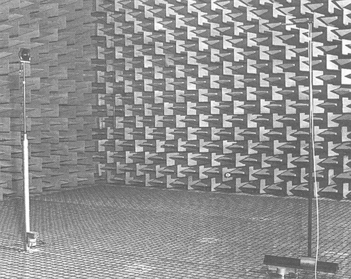

    

    Sound source (loudspeaker) and microphone located in an anechoic chamber

    Fig. 12.43

    

    Swim bladder anatomy

    Fig. 12.44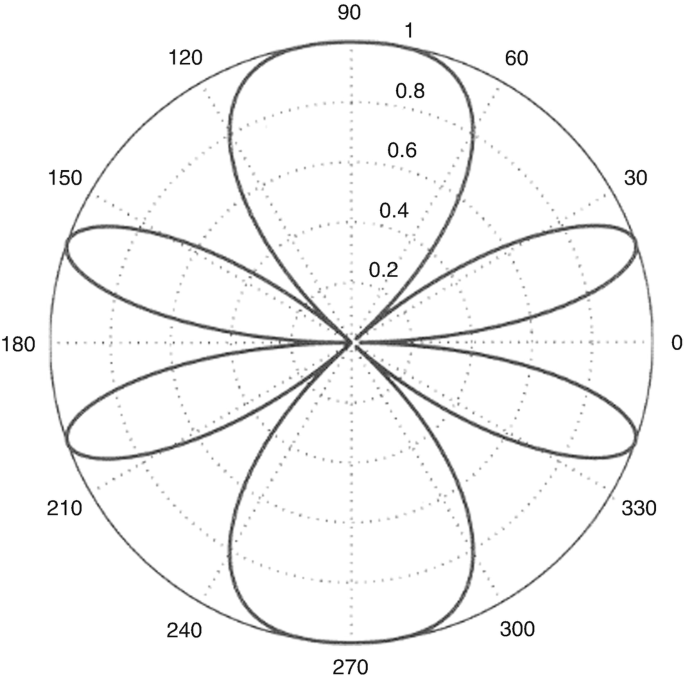

    

    Directional pattern for two sound sources of equal amplitude separated by a distance, d, between their centers

    Fig. 12.45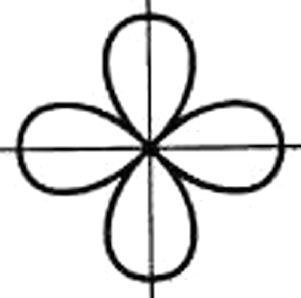

    

    Directional pattern for a four-element line array

    Fig. 12.46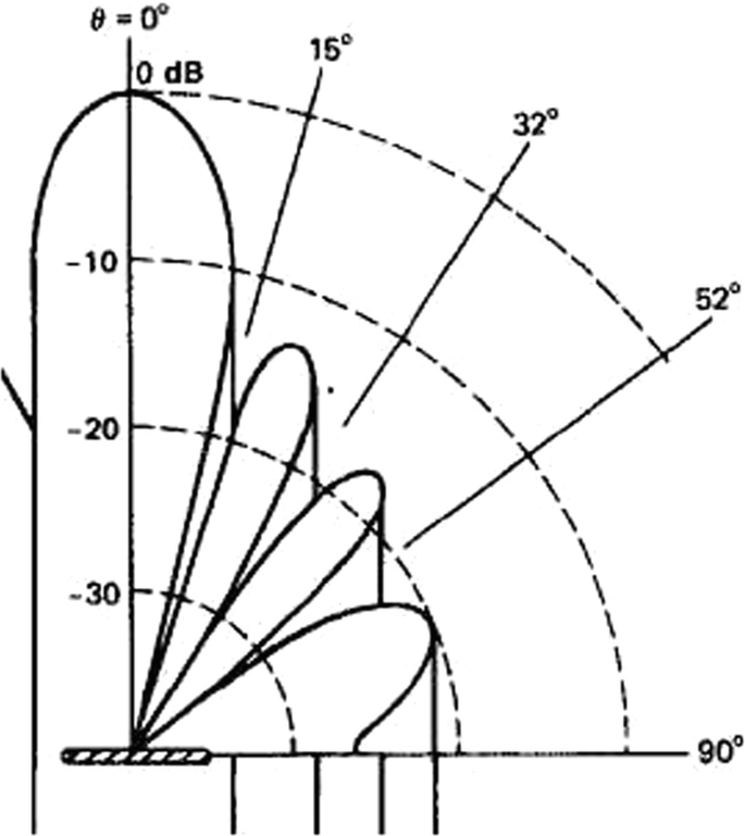

    

    Directional pattern of a continuous line array

    Fig. 12.47

    

    Quadratic quadrapole

    Fig. 12.48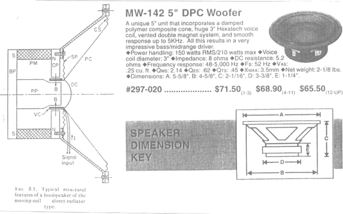

    

    (Left) Cross-section of a conventional moving-coil direct radiator type loudspeaker showing the suspension (CS), the spider (SP), speaker cone (PC), dust cap (DC), and voice coil (VC). The radial magnetic field (B) is produced by the permanent magnetic material (PM) with north (N) and south (S) magnetic polarity, the central pole piece (PP), the backplate (BP), and the front pole piece (CP). Figure from Hunt [65]. (Right) Catalog listing a 5” Morel model MW-142 loudspeaker

    Fig. 12.49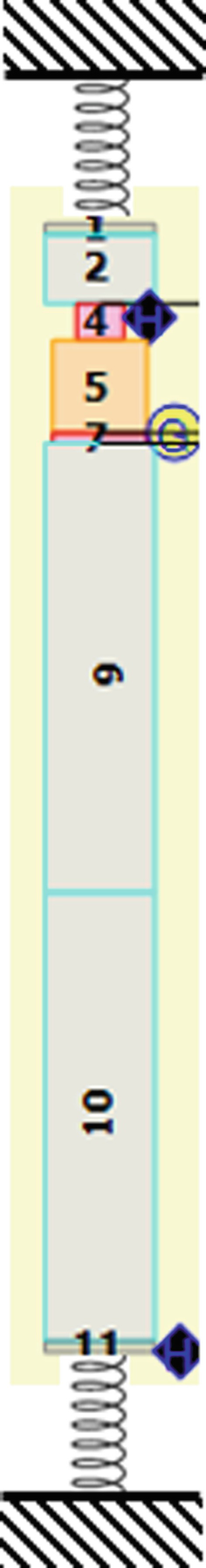

    

    Schematic representation of an elastically suspended thermoacoustic resonator

References

R. Weir, J. Garcia, D. Healy, R. Wickersham, Large room acoustics versus music. J. Acoust. Soc. Am. 58, S1 (1975)
B. Kinsman, Wind Waves: Their Generation and Propagation on the Ocean Surface (Prentice-Hall, Englewood Cliffs, 1965)
L.D. Landau, E.M. Lifshitz, Fluid Mechanics, 2nd edn. (Butterworth-Heinemann, Boston, 1987). See §15; ISBN:0-7506-2767-0. ISBN:0-7506-2767-0
V. Mangulis, Relation between the radiation impedance, pressure in the far field, and baffle impedance. J. Acoust. Soc. Am. 36, 212–213 (1964)
P.M. Morse, Vibration and Sound, 2nd edn. (McGraw-Hill, New York, 1948). See §27. Reprinted by the Acoust. Soc. Am., 1995; ISBN:0-88318-876-7
L.D. Landau, E.M. Lifshitz, Fluid Mechanics, 2nd edn. (Butterworth-Heinemann, Boston, 1987). §61; ISBN:0-7506-2767-0
M. Minnaert, Musical air bubbles and the sounds of running water. Philos. Mag. 16, 235–248 (1933)
M. Strasberg, The pulsation frequency of nonspherical gas bubbles in liquids. J. Acoust. Soc. Am. 25(3), 536–537 (1953)
T.F. Argo IV, P.S. Wilson, V. Palan, Measurement of the resonance frequency of single bubbles using a laser Doppler vibrometer. J. Acoust. Soc. Am. 123(6), EL212–EL125 (2008)
K.W. Commander, A. Prosperetti, Linear pressure waves in bubbly liquids: comparison between theory and experiments. J. Acoust. Soc. Am. 85(2), 732–746 (1989)
C. Devin Jr., Survey of thermal, radiation, and viscous damping of pulsating air bubbles in water. J. Acoust. Soc. Am. 31(12), 1654–1667 (1959)
O.B. Wilson, An Introduction to the Theory and Design of Sonar Transducers (Peninsula, Los Altos, 1989). ISBN:978-0932146229
R.L. Prichard, Mutual acoustic impedance between radiators in an infinite rigid plane. J. Acoust. Soc. Am. 32(6), 730–737 (1960)
S. Hanish, A Treatise on Acoustic Radiation, Vol. IV – Mutual Radiation Impedance and Other Special Topics (Naval Research Lab, Washington, DC, 1987)
T. Young, The Bakerian Lecture [1803]: experiments and calculations relative to physical optics. Phil. Trans. R. Soc. London 94, 1–16 (1804)
A. Howie, J.E. Ffowcs-Williams, Preface. Phil. Trans. R. Soc. London A360, 805–806 (2002)
J. Cui, M.F. Hamilton, P.S. Wilson, E.A. Zabolotskaya, Bubble pulsations between parallel plates. J. Acoust. Soc. Am. 119(4), 2067–2072 (2006)
A.D. Pierce, Acoustics: An Introduction to Its Physical Principles and Applications (McGraw-Hill, New York, 1981), pp. 482–486; ISBN:0-07-049961-6. Also reprinted by the Acoustical Society of America, 3rd ed. 2019; ISBN 978-3-030-11214-1
W.R. Smythe, Static and Dynamic Electricity (McGraw-Hill, London, 1939). §5.08
J.D. Jackson, Classical Electrodynamics (Wiley, New York, 1962). See Prob. 5.8
L.D. Landau, E.M. Lifshitz, Fluid Mechanics, 2nd edn. (Butterworth-Heinemann, Boston, 1987). §11; ISBN:0-7506-2767-0
P.M. Morse, K.U. Ingard, Theoretical Acoustics (McGraw-Hill, New York, 1968). §7.1
A.U. Case, The vocal microphone: technology and practice. Phys. Today 69(3), 74–75 (2016)
B. Baumzweiger, Microphone apparatus, US Patent No. 2,184,247, 19 Dec 1939
M.S. Pettersen, 75th anniversary of the Shure Unidyne® microphone. J. Acoust. Soc. Am. 136(4), 2129 (2014)
W.L. Dooley, Ribbon microphones. J. Acoust. Soc. Am. 136(4), 2130 (2014)
L.L. Beranek, Acoustics (Acoustical Society of America, New York, 1996). See Part XVI, §6.7; ISBN:0-88318-494-X
T.B. Gabrielson, Theory of operation for the DIFAR flux-gate compass. Naval Air Development Center Technical Memorandum 3031-86-02, April 1986
D.A. Brown, Bearing measurements using a compact wideband sensor by forming three dipoles. J. Acoust. Soc. Am. 134(5), 4052 (2013). Also see D.A. Brown, B. Aronov, C.L. Bachand, Acoustic transducers for underwater navigation and communication. U.S. Patent No. 8,638,640, 28 Jan 2014. Fig. 10A
R.M. Keolian, S.L. Garrett, C.B. Cameron, Demodulators for optical fiber interferometers with [3 X 3] outputs. U.S. Patent No. 5,313,266, 17 May 1994. See Fig. 17
S. Tempkin, Elements of Acoustics (Wiley, New York, 1981). See §5.5; ISBN:0-471-05990-0
L.D. Landau, E.M. Lifshitz, Fluid Mechanics, 2nd edn. (Butterworth-Heinemann, Boston, 1987). §74, see Problem 1; ISBN:0-7506-2767-0
T.B. Gabrielson, D.L. Gardner, S.L. Garrett, A simple neutrally-buoyant sensor for direct measurement of particle velocity and intensity in water. J. Acoust. Soc. Am. 97(4), 2227–2237 (1995)
L.D. Landau, E.M. Lifshitz, Fluid Mechanics, 2nd edn. (Butterworth-Heinemann, Boston, 1987). For an alternative derivation see §11, Problem 1; ISBN:0-7506-2767-0
S.L. Garrett, D.L. Gardner, Multiple axis fiber optic interferometric seismic sensor. U.S. Patent No. 4,893,930, 16 Jan 1990
D.L. Gardner, S.L. Garrett, A fiber optic interferometric seismic sensor with hydrophone applications. U.S. Navy J. Underw. Acoust. JUA(USN) 38(1), 1–21 (1988)
J.W. Strutt (Lord Rayleigh), On the light from the sky, its polarization and colour. Philos. Mag. XLI, 107–120 and 274–279 (1871); Scientific Papers, Vol. I (Dover, 1964) §8
J.W. Strutt (Lord Rayleigh), On the scattering of light from small particles. Philos. Mag. XLI, 447–454 (1871); Scientific Papers, Vol. I (Dover, 1964) §9
H. Lamb, The Dynamical Theory of Sound, 2nd edn. (Arnold, London, 1925). §79. Reprinted by Dover, 1960
T.G. Leighton, The Acoustic Bubble (Cambridge University Press, Cambridge, 1994). ISBN:0-12441-920-8. See §4.1.2
A. Mallock, The damping of sound in frothy liquids. Proc. R. Soc. A 84(572), 391–395 (1910)
F.S. Crawford, The hot chocolate effect. Am. J. Phys. 50(5), 398–404 (1982)
D. Fitzpatrick, J. Kruse, B. Vos, O. Foley, D. Gleeson, E. O’Gorman, R. O’Keefe, Principles and Application of Broadband Acoustic Resonance Dissolution Spectroscopy (BARDS): a sound approach for the analysis of compounds. Anal. Chem. 84, 2202–2210 (2012)
R.V.G. Peddapatla, M. Rizwan Ahmed, C.A. Blackshields, M.J. Sousa-Gallagher, S. McSweeney, J. Kruse, A.M. Crean, D. Fitzpatrick, Broadband Acoustic Resonance Dissolution Spectroscopy (BARDS): a novel approach to investigate the wettability of pharmaceutical power blends. Mol. Pharm. 15, 31–39 (2018)
I.S. Gradshteyn, I.M. Ryzhik, Tables of Integrals, Series, and Products, 4th edn. (Academic, London, 1980). See Eq. (0.112); ISBN:0-12-294760-6
K.U. Ingard, Fundamentals of Waves and Oscillations (Cambridge University Press, Cambridge, 1988). ISBN:0-521-33957-X
M. Abramowitz, I.A. Stegun, Handbook of Mathematical Functions with Formulas, Graphs, and Mathematical Tables, National Bureau of Standards, Applied Mathematics Series #55. p. 360, Eq. 9.1.20
M. Abramowitz, I.A. Stegun, Handbook of Mathematical Functions with Formulas, Graphs, and Mathematical Tables, National Bureau of Standards, Applied Mathematics Series #55. p. 360, Eq. 9.1.30
L.L. Beranek, Acoustics (Acoustical Society of America, New York, 1996). See Part X, §4.3; ISBN:0-88318-494-X
M. Abramowitz, I.A. Stegun, Handbook of Mathematical Functions with Formulas, Graphs, and Mathematical Tables, National Bureau of Standards, Applied Mathematics Series #55. p. 409, Table 9.5: Zeros and Associated values of Bessel Functions and Their Derivatives
I.S. Gradshteyn, I.M. Ryzhik, Tables of Integrals, Series, and Products, 4th edn. (Academic, London, 1980). p. 446, Eq. 3.821(9); ISBN:0-12-294760-6
P.M. Morse, K.U. Ingard, Theoretical Acoustics (McGraw-Hill, New York, 1968), pp. 383–387
M. Abramowitz, I.A. Stegun, Handbook of Mathematical Functions with Formulas, Graphs, and Mathematical Tables, National Bureau of Standards, Applied Mathematics Series #55. Chapter 12: Struve Functions and Related Functions, p. 496ff
R.M. Aarts, A.J.E.M. Janssen, Efficient approximation of the Struve function in the calculation of sound radiation quantities. J. Acoust. Soc. Am. 140(6), 4154–4160 (2016)
P.M. Morse, U.K. Ingard, Theoretical Acoustics (McGraw-Hill, New York, 1968). See Eq. (7.4.45)
M. Greenspan, Piston radiator: some extensions of the theory. J. Acoust. Soc. Am. 65(3), 608–621 (1979)
R.H. Mellen, M.B. Moffett, A model for parametric sonar radiator design. U. S. Navy J. Underw. Acoust. 22, 105–116 (1972)
H.M. Merklinger, High intensity effects in the non-linear acoustic parametric end-fire array. Ph.D. thesis, University of Birmingham, 1971
D.T. Blackstock, Fundamentals of Physical Acoustics (Wiley, New York, 2000). Chapter 13, §C; ISBN:0-471-31979-1
H. Levine, J. Schwinger, On the radiation of sound from an unflanged circular pipe. Phys. Rev. 73(4), 383–406 (1948)
J.W. Strutt (Lord Rayleigh), Theory of Sound, vol II, 2nd edn. (Macmillan, London, 1896). (Dover, 1945). §314 and App. A
L. Gutin, Uber das Schallfeld der Kolbenstrahlern. Tech. Phys. USSR 4, 404 (1937). Note that this is a German translation of an article that originally appeared in Russian
J.B. Mehl, Greenspan acoustic viscometer: numerical calculation of fields and duct-end effects. J. Acoust. Soc. Am. 106(1), 73–82 (1999)
N.A.M. Schellart, A.N. Popper, Functional aspects of the evolution of the auditory system in Actinopterygian fish, in The Evolutionary Biology of Hearing, ed. by D. B. Webster, R. R. Fay, A. N. Popper, (Springer, New York, 1992), pp. 295–322
F.V. Hunt, Electroacoustics (Harvard University Press, Cambridge, MA, 1954). See Fig. 5.1
S.L. Garrett, J.A. Smith, R.W.M. Smith, B.J. Heidrich, M.D. Heibel, Fission powered in-core thermoacoustic sensor. Appl. Phys. Lett. 108, 144102 (2016). Using the sound of nuclear energy. Nucl. Technol. 195(3), 353–362 (2016)
Author information
Authors and Affiliations
Rights and permissions
Open Access This chapter is licensed under the terms of the Creative Commons Attribution 4.0 International License (http://creativecommons.org/licenses/by/4.0/), which permits use, sharing, adaptation, distribution and reproduction in any medium or format, as long as you give appropriate credit to the original author(s) and the source, provide a link to the Creative Commons license and indicate if changes were made.
The images or other third party material in this chapter are included in the chapter's Creative Commons license, unless indicated otherwise in a credit line to the material. If material is not included in the chapter's Creative Commons license and your intended use is not permitted by statutory regulation or exceeds the permitted use, you will need to obtain permission directly from the copyright holder.
Copyright information
© 2020 The Author(s)
About this chapter
Cite this chapter
Garrett, S.L. (2020). Radiation and Scattering. In: Understanding Acoustics. Graduate Texts in Physics. Springer, Cham. https://doi.org/10.1007/978-3-030-44787-8_12
Download citation
DOI: https://doi.org/10.1007/978-3-030-44787-8_12
Published:
Publisher Name: Springer, Cham
Print ISBN: 978-3-030-44786-1
Online ISBN: 978-3-030-44787-8
eBook Packages: Physics and AstronomyPhysics and Astronomy (R0)