
Abstract
Having already invested in understanding both the equation of state and the hydrodynamic equations, only straightforward algebraic manipulations will be required to derive the wave equation, justify its solutions, calculate the speed of sound in fluids, and derive the expressions for acoustic intensity and the acoustic kinetic and potential energy densities of sound waves. The “machinery” developed to describe waves on strings will be sufficient to describe one-dimensional sound propagation in fluids, even though the waves on the string were transverse and the one-dimensional waves in fluids are longitudinal. These results are combined with the thermal and viscous penetration depths to calculate the frequencies and quality factors in standing wave resonators. The coupling of those resonators to loudspeakers will be examined. The introduction of reciprocal transducers that are linear, passive, and reversible will allow absolute calibration of transducers using only electrical measurements (i.e., currents and voltages) by the reciprocity method, if the acoustic impedance that couples the source and receiver is calculable. Reflection and transmission at junctions between multiple ducts and other networks will be calculated and applied to the design of filters. The behavior of waves propagating through horns will provide useful impedance matching but introduce a low-frequency cut-off.
You have full access to this open access chapter, Download chapter PDF
Keywords
- Sound speed
- Dispersion relation
- Characteristic impedance
- Decibel
- Reciprocity calibration
- Exponential horns
Having already invested in understanding both the equation of state in Chap. 7 and in the hydrodynamic equations in Chap. 8, only straightforward algebraic manipulations will be required to derive the wave equation, justify its solutions, calculate the speed of sound in fluids, and derive the expressions for acoustic intensity and the acoustic kinetic and potential energy densities. The “machinery” developed to describe waves on strings will be sufficient to describe one-dimensional sound propagation in fluids, even though the waves on the string were transverse and the one-dimensional waves in fluids are longitudinal.
Most treatments of one-dimensional propagation in acoustics courses start their discussion of waves in fluids at this point (possibly treating lumped-element systems later), but with our understanding of the fundamental phenomenological equations already established for lumped elements, we will be able to take a more rigorous approach that will also allow incorporation of other effects that can be combined with the dissipative effects introduced in Chap. 9, particularly for calculation of the attenuation of sound in Chap. 14. Also, having examined combinations of inertances and compliances, the transition from lumped fluid elements to waves in fluids is philosophically identical to the transition from coupled simple harmonic oscillators to waves on strings.
1 The Transition from Lumped Elements to Waves in Fluids
The equation of state, as exemplified by the adiabatic gas law of Eq. (7.20), and the linearized versions of the continuity equation combined with the adiabatic gas law in Eq. (8.23) were used to create lumped compliances in Sect. 8.2.3. The linearized version of the Euler Eq. (8.40) was used to create lumped inertances, and then both inertance and compliance were applied to fluid elements that were small compared to the wavelength of sound in Sect. 8.4.3. Those equations can now be extended to continuous fluid media in systems that are substantial fractions of a wavelength or larger.
Since the lumped-element model was linear, we are free to combine solutions. Although the neck of our Helmholtz resonator in Sect. 8.5.2 was represented entirely by its inertance (gas mass) and the spherical volume was represented entirely by its compliance (gas stiffness), in general, a single “lumped” element could simultaneously exhibit both properties by linear superposition. If there are changes in the volume velocity of the fluid entering and leaving the element, ΔU, as well as a pressure difference, Δp, across an element, like those diagrammed schematically in Figs. 8.3 and 8.8, then the element would exhibit both inertance (due to Δp) and compliance (due to ΔU).
In this chapter, we will expand our focus to include acoustical systems with characteristic dimensions comparable to, or longer than, the wavelength of sound in the fluid. These can also be modeled using lumped parameters, if we employ enough elements. For instance, a resonator with diameter that is a small fraction of the wavelength, but a length that is equal to one-half of the wavelength of sound, can be modeled as a sequence of compliances and inertances as depicted schematically in Fig. 10.1.

A half-wavelength resonator (above) of constant cross-sectional area with rigid ends is approximated as a series of seven lumped compliances and six lumped inertances. The elements near the ends contribute primarily compliance since the longitudinal motion of the fluid must vanish at the boundary (velocity nodes). Most of the energy stored near the ends is compressive (potential). The central elements contribute mostly inertance since the fluid velocity at the center is largest (near the velocity anti-node). Most of the energy within the central pair of inertances is kinetic. In fact, the approximation is nearly as good if the central compliance is removed from the model (but only for the fundamental half-wavelength mode!). The two pairs of elements that are intermediate between the two end elements and the central elements must provide both significant inertance and compliance
As demonstrated in Sect. 2.7.7, the behavior of standing waves on strings can be approximated by identical discrete masses coupled by identical lengths of a massless string under uniform tension. The fundamental mode of nine such coupled oscillators is shown in Fig. 2.30 to be a good approximation to the half-sinewave mode of a string, like that shown in Fig. 3.6. This approach has some significant utility if you are interested in studying systems with changing cross-section. As shown in Fig. 10.2, a horn of finite length, analyzed in Sect. 10.9.3, can be approximated by a series of stepped ducts of increasing cross-section.

A stepwise approximation to a horn. The number of elements is chosen so the area change between elements is small [1]
The broadband, omnidirectional sound source shown in Fig. 10.3 was designed to radiate sound uniformly in all directions and to give reproducible and reliable results for evaluation of building acoustics with a sufficient overall sound pressure level to provide adequate signal-to-noise ratios. The International Organization for Standardization (ISO) has published two standards for broadband sound sources that are used for architectural acoustical evaluations in buildings [2]. The standards require uniform levels, within a frequency-dependent number of decibels (see Sect. 10.5.1) in each of twenty-one 1/3-octave frequency bands (ISO 3382). The source must also radiate sound uniformly in all directions (ISO 140).

The Brüel & Kjær Type 4295 sound source was “carefully engineered to radiate sound evenly in all directions” by Dr. Jean-Dominique Polack. The source was designed to conform to the standard 1/3-octave band sound level and directionality requirements by using a resonator coupled to an electrodynamic loudspeaker. Although a resonator is about as far from a “broadband” sound source as one might possibly imagine, it does satisfy the standards as written
A very clever acoustician, Jean-Dominique Polack,Footnote 1 realized that he could design a very simple source consisting of a single loudspeaker radiating out of a small aperture (to ensure omnidirectionality, as shown in Fig. 12.32a) that would be very compact and efficient by making a resonator and “tuning” the resonances within each 1/3-octave band (though not necessarily at the band center frequency). He did this by writing a finite element code that incorporated 28 lumped elements and then adjusted those elements to place the resonances within the 1/3-octave bands specified by ISO 3382.Footnote 2
At some point, it makes sense to model the entire resonator as a continuum just as it did in our transition from coupled simple harmonic oscillators to strings. We do that by specifying a continuous function that describes the pressure and fluid velocity at each point in space and time—a wave function.
2 The Wave Equation
Our study of the fundamental equations of hydrodynamics has provided us with a set of three Eqs. (7.32), (7.34), and (7.42) that describe the motion of any homogeneous, viscous, thermally conducting, and isotropic, single-component fluid. We supplemented those hydrodynamic equations by equations of state (7.49) and (7.50) that provide relationships among the mechanical variables (p and ρ) and thermodynamic variables (T and s) that appear in the hydrodynamic equations.
The linearized, one-dimensional, nondissipative versions of those equations are first-order partial differential equations that define relationships among different variables. For example, the continuity equation or mass conservation Eq. (8.17) relates changes in density to the divergence of the fluid velocity or mass flux. Similarly, the linearized one-dimensional Euler Eq. (8.40) relates changes in the velocity to gradients in the pressure. An equation of state, for example, (7.19), can relate changes in pressure to changes in density.
It is possible to combine those first-order partial differential equations to create a second-order partial differential equation for a single variable. To illustrate this process, let us start with a one-dimensional version of the linearized continuity Eq. (8.17), where we let vx = u = v1,
and the linearized one-dimensional Euler equation, where again vx = u = v1,
That set of two first-order coupled differential equations contains three (potentially complex) variables: ρ1, v1, and p1. To “close” the system, we need one additional equation to eliminate either p1 or ρ1. Closure can be achieved by invoking an equation of state. In this case, we will choose to express density in terms of pressure, ρ = ρ (p), which can be expanded in a Taylor series to eliminate ρ1 in favor of p1 in Eq. (10.1).
As was demonstrated in Sect. 9.3.4, at nearly all frequencies of interest in gases or liquids, sound propagation is adiabatic. For that reason, we have taken the derivatives of the density with respect to pressure in Eq. (10.3) while holding entropy per unit mass constant, as indicated by the subscript, s, on the partial derivatives. Since we are interested in the linearized result, we retain only the first term in the Taylor series of Eq. (10.3). As we will see shortly, it is convenient to name that derivativeFootnote 3 the reciprocal of the square of the speed of sound, c−2.
Substituting Eq. (10.4) into Eq. (10.1), we obtain,
Now Eqs. (10.2) and (10.5) constitute a pair of homogeneous first-order coupled differential equations in two variables. Those equations can be combined to eliminate either p1 or v1. Let us start by eliminating v1. That can be accomplished by multiplying the linearized Euler Eq. (10.2) by ρm and taking its derivative with respect to x.Footnote 4
We can then take the time derivative of the linearized continuity Eq. (10.5).
Since the order of differentiation is irrelevant, when Eq. (10.6) is subtracted from Eq. (10.7), we are left with a second-order, homogeneous, partial differential equation in only one variable.
The result in Eq. (10.8) is the well-known one-dimensional wave equation. It provides us with an expression that can relate the time and space dependence of p1(x, t). Since pressure and density deviations from equilibrium are related by the square of the sound speed, then we would obtain the same wave equation for ρ1.
If the combination process is reversed by taking the spatial derivative of the linearized continuity Eq. (10.5), we obtain,
Similarly, the linearized Euler Eq. (10.2) can be multiplied by ρm, and then the time derivative can be taken.
Once again, ignoring the order of differentiation, subtraction of Eq. (10.10) from Eq. (10.11) produces the wave equation for the linear contribution to the x component of the acoustic particle velocity, v1.
2.1 General Solutions to the Wave Equation
The wave equation, as written in Eq. (10.8) or Eq. (10.12), is a second-order partial differential equation. As such, it must have two linearly independent solutions: ya and yb. Of course, any one-dimensional, linear, wave equation will be isomorphic to the version that appeared first as the equation for propagation of transverse waves on a string in Eq. (3.4).
As was demonstrated in Sect. 3.1, it is not difficult to show that any arbitrary function having (ct ± x) in its argument is a solution. Whether c is the speed of sound in a fluid, or the speed of transverse waves on a string, f (ct ± x) are the solutions to Eq. (3.4) as well as Eqs. (10.8), (10.9), and (10.12). If we choose pressure as the variable that characterizes the amplitude of the sound wave, then the excess acoustic pressure due to the sound wave, p1(x, t), can be expressed as the superposition of the right-going and left-going waves.
As with our solutions for waves on strings, for purposes of computational convenience and conformity with physical reality for most acoustical systems, we employ the trigonometric functions, or complex exponential functions, or combinations of those functions as our solutions of choice for single-frequency waves, as we did for traveling waves.
Standing waves can be represented as the superposition of a right- and left-going traveling waves of equal amplitudes. Letting \( {\hat{\mathbf{p}}}_{\mathbf{left}}={Ae}^{-j\left({\phi}_t+{\phi}_x\right)}/2 \) and \( {\hat{\mathbf{p}}}_{\mathbf{right}}={Ae}^{-j\left({\phi}_t-{\phi}_x\right)}/2 \), with \( \overrightarrow{k}\cdotp \overrightarrow{x}= kx \), and making ℑm[A] = ℑm[ϕt] = ℑm[ϕx] = 0, Eq. (10.14) becomes,
As before, the scaling of time by angular frequency, ω, and position by wavenumber, k, is a particularly useful choice that makes the argument of the functions dimensionless.
The same functions could just as well have been written for the linear variations in the density, ρ1 (x, t), from its equilibrium value, ρm, or the variation in the particle velocity, v1 (x, t), where we have assumed vm = 0.
3 The Dispersion Relation (Phase Speed)
Once we have used the wave equation to demonstrate that the solutions for each variable that characterizes its linear deviation from equilibrium have wave-like space and time behavior, the wave equation does not provide any immediate additional utility. To demonstrate this fact, we can return to the coupled first-order linearized continuity Eq. (10.1) and Euler Eq. (10.2).
By using the complex notation of Eq. (10.14) with \( {\hat{\mathbf{p}}}_{\mathbf{left}}=0 \) to describe a single-frequency right-going propagating wave, differentiation with respect to time corresponds to a simple multiplication of p1 by +jω and differentiation with respect to position corresponds to a simple multiplication of p1 by –jk. Application of this convenience (aka complex) transformation (harmonic analysis) to the linearized continuity Eq. (10.5) yields,
Similarly, the linearized Euler Eq. (10.2) becomes,
This pair of linear coupled algebraic equations, (10.16) and (10.17), will only have a nontrivial solution if the determinant of their coefficients vanishes.
Evaluation of the determinant specified in Eq. (10.18) produces a relationship between ω and k that is known as a dispersion relation.
This result provides the definition of the phase speed, c ≡ ω /k, thus justifying the concepts of wavenumber, k; wavelength, λ; frequency, f; and period, T, that we have been using since Chap. 3: c = fλ = ω/k.
3.1 Speed of Sound in Liquids
The square of the adiabatic speed of sound is expressed as the thermodynamic derivative of pressure with respect to density in Eq. (10.4). For fluids, that result is related to another thermodynamic derivative; the adiabatic bulk modulus, Bs, has the same units as pressure:
In Sect. 4.2.1, the previous derivation for the bulk modulus in solids did not specify whether the modulus was evaluated under isothermal or adiabatic conditions since there is very little difference between those values for solids.
The adiabatic bulk modulus is the reciprocal of the adiabatic compressibility. By comparison of Eq. (10.20) to Eq. (10.4), we see that the adiabatic sound speed in a fluid can be expressed in terms of the adiabatic bulk modulus and the fluid’s mass density.
The form of Eq. (10.21) is typical of sound propagation speeds because it shows that the speed is determined by the ratio of a restoring “stiffness” to an inertial mass density.
The bulk modulus is an intensive material property. For most liquids, it is usually found in handbooks and can be a complicated function of both pressure and temperature. The expression for the speed of sound in seawater, given in Eq. (11.26), includes terms that are a function of salinity, as well as pressure [3]. Even a simple cryogenic liquid, such as liquid nitrogen (LN2), exhibits complicated pressure dependence of its sound speed:
where c is in [m/s] and p is in atmospheres (1 atm ≡ 101,325 Pa) [4].
3.2 Speed of Sound in Ideal Gases and Gas Mixtures
For an ideal gas, the form of the sound speed is particularly simple and universal. Logarithmic differentiation of the ideal gas adiabatic equation of state, pρ−γ = constant, immediately produces an expression for the speed of sound in an ideal gas, based on Eq. (10.4):
The Ideal Gas Law (7.4) allows Eq. (10.22) to be expressed in terms of the molecular (or atomic) mass of the gas, M; its absolute [kelvin] temperature, T; and the universal gas constant, ℜ:
It is worthwhile to reflect on the adiabatic sound speed for ideal gases as expressed in Eq. (10.23) for several reasons: First, it demonstrates that the sound speed in an ideal gas is not a function of pressure. This is not obvious from Eq. (10.22), which could (naïvely) be interpreted to imply that the sound speed increases with the square root of pressure. This is incorrect, because the ratio of pressure to density depends only upon absolute [kelvin] temperature, polytropic coefficient, and molecular weight.
Equation (10.23) also highlights the fact that the sound speed is proportional to the square root of absolute [kelvin] temperature. As of 20 May 2019, the international standard absolute temperature scale is based on sound speed measurements [5], just as the exact value of Boltzmann’s constant, kB ≡ 1.380649 × 10⁻²³J/K, and the universal gas constant, ℜ ≡ kBNA ≡ 8.314462 J/mole-K, has been tied to sound speed measurements since the mid-1980s [6].
The third reason that Eq. (10.23) is important is that it provides a means of calculating the speed of sound in gas mixtures. If we have a binary mixture of ideal gases with a concentration, x, of one species with molecular mass, M1, and concentration, (1 – x), of the second species with molecular mass, M2, then the mean molecular mass of the gas mixture, Mmix, is simply their concentration-weighted average:
This expression can be generalized to mixtures, such as air, with more than two constituents (see Table 10.1).
Since the polytropic coefficient, γ = cp/cV, also known as the ratio of specific heats, is an intensive quantity, it is not correct to calculate γmix as a weighted average of the individual polytropic coefficients, although it is not too bad an approximation in some circumstances [7], since the range of γ is limited: 1 < γ ≤ 5/3. To calculate γmix correctly, the heat capacities are averaged:
This result can be written in another form if the concentration weighting is applied to the reciprocals of (γ – 1) [8].
A similar approach can be used to estimate the transport coefficients in gas mixtures: thermal conductivity, viscosity, and Prandtl number, as was done in Sect. 9.5.4 [9].
Since the sound speed is independent of pressure and the temperature dependence can be easily compensated, being proportional to the square root of absolute temperature,Footnote 5 it is possible to build sonic gas analyzers that determine the concentration of a contaminant quickly, accurately, and inexpensively [12, 13]. The helium contamination alarm, shown schematically in Fig. 10.4, uses the variation in sound speed to detect leakage of air into a helium gas recovery system [14]. Other more sophisticated systems have been developed that allow flow-through measurement with differential processing to increase common-mode rejection of flow and environmental noise [12, 15].

The cylindrical plane wave resonator in the upper left corner of this block diagram is closed at each end by electret (12 μm thick aluminized Teflon®) transducers (see Sect. 6.3.3) [16]. One electret transducer is used as a microphone and the other as a speaker. A slot at the resonator’s midplane allows the resonator to sample the helium gas flowing through the recovery line without degrading the resonator’s quality factor. The system is maintained at its fundamental resonance frequency by applying the amplified microphone output to the speaker through an inductor tuned to the electret speaker’s electrical capacitance. (In a public address system, this would be considered feedback squeal.) A 37 m coil of #44 copper wire (RT ≅ 350 Ω) is epoxied to the resonator and is used as a thermometer. A frequency-to-voltage conversion (tachometer) chip [17] produces a dc voltage proportional to the resonance frequency that is summed with the temperature-dependent voltage produced by RT along with an offset voltage that is adjusted when pure helium gas is in the recovery line. If air enters the recovery line, the frequency decreases, and an alarm is activated and the recovery valve is closed [14]
4 Harmonic Plane Waves and Characteristic Impedance
The linearized first-order Euler Eq. (10.2) can be solved to relate the acoustic fluid (particle) velocity, v1, to the acoustic pressure, p1. For a harmonic, one-dimensional plane traveling wave, expressed in Eq. (10.14), the ratio of pressure to particle velocity is z, remembering that c = ω /k.
This property of a fluid is sufficiently important to be given its own name: the specific acoustic impedance or the characteristic impedance. The units of specific acoustic impedance are Pa-s/m, also called the rayl (sometimes the MKS rayl to distinguish it from the cgs rayl), in honor of the third Lord Rayleigh (J. W. Strutt, 1842–1919).
Another short digression regarding the three impedances used in acoustics is beneficial at this point. We have previously encountered an impedance that we called the acoustic impedance. It was defined as the ratio of the pressure to the volume velocity at one location: \( {\mathbf{Z}}_{\mathbf{ac}}=\hat{\mathbf{p}}/\hat{\mathbf{U}} \). That impedance was particularly useful for describing systems that join elements with differing cross-sectional areas (e.g., Helmholtz resonator) to ensure the continuity of mass flow. We will also see that another version, the acoustic transfer impedance, Ztr, will be very useful in problems that involve acoustic radiation and transduction (see Sect. 10.7). The acoustic transfer impedance is given by the pressure at one location (the receiver) divided by the volume velocity produced at the source of sound.
In Eq. (10.27), we have just defined a specific acoustic impedance, the ratio of pressure to particle velocity, which is a property of the acoustic medium and is independent of geometry. It is especially useful in the description of plane waves, particularly when they impinge on boundaries between media with different properties, as will be addressed in detail in Chap. 11. The third impedance is the mechanical impedance, \( {\mathbf{Z}}_{\mathbf{mech}}=\hat{\mathbf{F}}/\hat{\mathbf{v}} \). The mechanical impedance is useful for determining the steady-state response of a vibro-mechanical network.
Frequently in acoustics, and particularly for problems involving transduction, these different complex impedances (as well as the electrical impedance, \( {\mathbf{Z}}_{\mathbf{el}}=\hat{\mathbf{V}}/\hat{\mathbf{I}} \)) need to be combined to couple an electromechanical system to an acoustical medium. It is easy to relate the three impedances for a system with a characteristic cross-sectional area, A.
In Eq. (10.28), the pressure amplitude, \( \hat{\mathbf{p}} \); volume velocity amplitude, \( \hat{\mathbf{U}} \); and particle velocity amplitude, \( \hat{\mathbf{v}} \), were all complex phasors to emphasize the fact that impedance is a concept that is based on linear acoustics and the assumption of a single-frequency wave-like disturbance from equilibrium.
The specific acoustic impedance, z = ρmc, is convenient for representing the space and time dependence of the acoustic fluid (particle) velocity, v1(x, t), for a traveling wave moving in the positive x direction. Below, Eq. (10.29) has ±ρmc in the denominator to remind us that a wave traveling in the minus x direction would have a negative specific acoustic impedance.
The continuity equation can be used to relate density variations, ρ1(x, t), to the particle velocity, v1(x, t), of a plane wave with the final version restricted to a single-frequency wave.
The dot product that appears in the spatial dependence within the argument of the exponential functions in Eqs. (10.14) and (10.29) can be expanded into its Cartesian components for an arbitrary choice of directions with respect to the Cartesian axes.
Normally, if a plane wave is propagating in an arbitrary direction, it is easier to re-orient the coordinate axes so that one axis is along the direction of propagation and the one-dimensional expressions will suffice. In an isotropic medium, the wave vector, \( \overrightarrow{k} \), defines a direction that is perpendicular to the wave’s planes of constant phase.
5 Acoustic Energy Density and Intensity
Since our hydrodynamic equations provide a complete description of the fluid, there should be no need to introduce any additional equations to account for the energy density of the fluid or for the acoustical energy transported by the waves. For the nondissipative case, that fact can be demonstrated by combining the continuity equation and the Euler equation in another way.
We start by writing the linearized three-dimensional vector form of the continuity Eq. (8.9), augmented by the equation of state (10.4), as expressed in the one-dimensional version in Eq. (10.5).
The continuity equation can be combined with the linearized three-dimensional vector form of the Euler equation.
If we take the dot product of \( {\overrightarrow{v}}_1 \) with Eq. (10.33) and multiply Eq. (10.32) by p1 and add the two equations together, we can collect terms if we notice that the product rule (see Sect. 1.1.2) produces the following identities:
We can also exploit the vector version of the product rule for differentiation (see Sect. 1.1.2).
The combination can be expressed as a conservation equation for acoustic energy.
As was established in Sect. 7.3.1, when the continuity Eq. (7.32) was first introduced, Eq. (10.36) has the form of a conservation equation: it is the time derivative of a density plus the divergence of a flux. It is easy to identify the \( \left(\frac{1}{2}\right){\rho}_m{v}_1^2 \) term in Eq. (10.36) as the kinetic energy density of the sound wave; therefore \( \left(\frac{1}{2}\right){p}_1^2/{\rho}_m{c}^2 \) must be the potential energy density. In this case, the corresponding flux is the acoustic intensity, I.
The energy densities and the intensity are quadratic combinations of first-order acoustic variables. The two energy densities within the square brackets in Eq. (10.36) are positive-definite quantities. Why do we not neglect these second-order quantities when, up to this point, we have discarded all second-order quantities? In this case, this second-order quantity is the leading-order contribution. When we linearized other equations, there were linear terms that dominated second-order terms, typically by a factor of Mac, for example, in Eqs. (8.18) and (8.19). For energetic variables (e.g., energy density, intensity, enthalpy flux), there are no first-order contributions in the absence of steady flow.
In the presence of dissipation, the acoustical energy is not conserved, and Eq. (10.36) would no longer be homogeneous, although it would have the same form:
In Eq. (10.38), E is the energy density, \( \overrightarrow{I} \) is the (vector) intensity, and D is a dissipation factor [18].
The (irreversible) dissipation created by the shear viscosity, μ, and the thermal conductivity, κ, should be familiar from the expressions for boundary-layer losses provided in Eq. (9.34). The first term in Eq. (10.39) introduces a new “viscosity,” ζ, which is called a “bulk viscosity” (or also called “second viscosity”). As will be discussed in Sect. 14.5, the bulk viscosity has been added to account for relaxation absorption (e.g., the fact that it takes some non-zero time for the Equipartition Theorem to distribute energy equitably between translational and rotational degrees of freedom) [19]. The second term in Eq. (10.39), proportional to the thermal conductivity, κ, is obviously thermal loss, since it contains (γ − 1)/γ as a coefficient and is proportional to the square of the acoustic pressure. The final term arises from (rotational) flow with non-zero curl, such as the shear produced in the viscous boundary layer that was calculated in Sect. 9.4.3.
5.1 Decibel Scales
The Bell Telephone Laboratories developed much of the “modern” (twentieth-century) science of acoustics and its implementation in engineering practice. For almost a century, Bell Telephone (renamed AT&T in 1899) enjoyed a telecommunications monopoly within the United States. This allowed the company to recoup its investment in equipment and capital improvements like buildings, poles, purchased right-of-way, etc. Eventually (1913), the US Government put a cap on Bell’s profits, limiting them to 10% after taxes. To operate under this lower margin, Bell invested “excess profits” by spending them on research and development within two of its subsidiaries: Bell Laboratories and Western Electric. Despite this cap on profits, Bell became one of the most successful companies in the history of the world. It was the largest US corporation until a forced divestiture was imposed by the US Congress in 1984.
Most of us are more familiar with the later Nobel Prize winning research accomplishments of Bell Labs. The best-known of these is the invention of the transistor (Bardeen, Brittan, and Shockley, 1947) and the invention of the laser (Schawlow and Townes, 1948). Also credited to Bell Lab scientists are the discovery of local electronic states in solids (Anderson Localization, 1977) and the discovery of the 4 K residual cosmic black-body background radiation left over from the “Big Bang” (Penzias and Wilson, 1978), as well as acoustical engineering advances that did not receive the Nobel, such as the electret microphone (Sessler and West 1964). More recent Nobel Prizes include optical trapping (Chu 1997)Footnote 6 and the quantum Hall effect (Stormer 1998).
During the interval between the two world wars, many of the engineering concepts we use today evolved from research at Bell Labs that were directed toward the commercialization of a worldwide telecommunication network. The later research involved major advances in digital electronics including the “sampling theorem” of Claude Shannon (1948), the concept of digital filters introduced by R. W. Hamming (1977), and the fast Fourier transform by John Tukey (1965), along with the development of the UNIX operating system (1971). Before the advent of digital electronics, Bell Labs did the systems engineering that started with the characterization of vocalization and auditory perception (Fletcher and Munson, see Fig. 10.5) and carried through with the competition between transmission loss and amplificationFootnote 7 required to transmit human voices around the world. The focus on the competition between amplifier gain and transmission loss led to the introduction of the decibel.

The equal-loudness contours, known as the Fletcher-Munson curves, are taken from [21]. The solid lines correspond to the intensity of sound in air, in dB re: 1 pW/m2, which is required to produce a perceived loudness equal to that of a 1.0 kHz tone with the same intensity level. That “loudness level” is called the “phon.” To produce a loudness level of 60 phon, at 1.0 kHz, the sound pressure level would be 60 dBSPL. The “0 dB” curve is often called the “threshold of hearing,” and the “120 dB” curve is called the “the threshold of feeling”
The decibel (abbreviated dB) was introduced by Bell Labs engineers to quantify the reduction in audio level over a 1-mile length of standard telephone cable. It was originally called the transmission unit, or TU, but was renamed in 1923 or 1924 in honor of the laboratory’s founder and telecommunications pioneer, A. G. Bell. Before the days of hand-held electronic calculators, it was easier to add or subtract logarithms than it was to multiply long strings of gain and loss factors.
Although there are periodic debates about whether or not to dispose of the decibel, in acoustics it is unlikely that the decibel will disappear during the span of your career [20]. One reason for the decibel’s persistence into the age of digital electronics is physiological. The dynamic range of human hearing covers about 14 orders of magnitude in intensity. In some sense, sound pressure levels expressed in decibels provide a “centigrade scale” for sound levels that nicely matches human auditory experience; 0 dBSPL is about the quietest sound a human can detect, and 100 dBSPL is about as loud a sound as we can tolerate.
By far, the most important feature of the decibel is that the decibel is always a base-10 logarithmic measure of a ratio, never a ratio itself.
The intensity level, IL, is expressed in decibels.
The time-averaged acoustic intensity, I = <p1v1 > t, is defined by the energy conservation Eq. (10.36). The time-averaged reference intensity, Iref, used to define IL in Eq. (10.40), will depend upon the situation. For sound in air, Iref ≡ 10−12 W/m2 = 1 pW/m2. Using our definition of specific acoustic impedance for plane waves in Eq. (10.27), the value of the specific acoustic impedance in dry air is z = ρmc = 413.3 Pa-sec/m (rayls) at 20 °C, so Iref can also be expressed in terms of the root-mean-squared pressure, prms, of sound.
In Eq. (10.41), we let \( {p}_{rms}={p}_1/\sqrt{2} \) by assuming that the pressure was varying sinusoidally in time.Footnote 8 If that is the case, then Iref corresponds to a root-mean-squared pressure amplitude, prms = 20.33 μParms. For convenience, the reference sound pressure in air is defined as Pref ≡ 20 μParms.
The concept of sound pressure level, expressed in decibels, appeared in Chap. 7 to describe the amplitude of a dangerously loud sound: 115 dBSPL.
The fact that the base-ten logarithm in Eq. (10.42) is multiplied by 20 instead of 10, as in Eq. (10.40), reflects the definition of the decibel as the base-10 logarithm of a power or intensity ratio, even when its value is determined by the ratio of amplitudes.
If the decibel is used to express an amplitude-independent ratio (like the gain of an amplifier or the attenuation of a filter), then a reference level is not required, but the ratio must still be the logarithm of a power or energy ratio. For example, if the voltage gain of an amplifier is ten, then that gain can be expressed as 20log10(10) = + 20 dB.
When a decibel refers to an absolute measurement, then it is important to include the reference along with the reported value. That can be accomplished in several ways. One is the subscript used for 115 dBSPL that implied that Pref = 20 μParms for sound pressure levels (SPL). The preferred method is always to explicitly include the reference: 115 dB re: 20 μParms.
There are several frequency-weighting schemes that are used to produce a dB level that reflects the (amplitude-dependent!) frequency response of human hearing that will be addressed in Sect. 10.5.3.Footnote 9 For example, an A-weighted sound pressure level (LA) can be expressed as 115 dB(A) or 115 dBA.
5.2 Superposition of Sound Levels (Rule for Adding Decibels)
As just mentioned, the decibel was introduced to turn a multiplicative string of gains and losses into an arithmetic sum. When it comes to the superposition of sound fields, the decibel must be employed with extreme care!
If we add two sound sources, each with a sound pressure level of 60 dBSPL, the result is either 63 dBSPL if the sources are incoherent, since their powers add, or as much as 66 dBSPL if the sources are coherent (having the same frequency) and in-phase, since their pressures would add. If the sources are coherent and out-of-phase, there may be no sound at all. In no case will the sum of two 60 dBSPL sources ever result in 120 dBSPL!
5.3 Anthropomorphic Frequency Weighting of Sound Levels
It is common to assert that healthy humans can detect sound with frequencies ranging from 20 Hz to 20 kHz, but the sensitivity of human hearing is very dependent upon both frequency and amplitude, as well as on the listener’s age, health, and prior exposure to loud sounds. The frequency dependence of human hearing is represented by equal-loudness contours that were first measured by Fletcher and Munson at Bell Labs in 1933 [21]. Subsequent determinations were made to produce equal-loudness contours that specified the auditory acuity of different age groups [22], and consensus contours have been codified in an international standard [23]. For our present purposes, the Fletcher-Munson curves, shown in Fig. 10.5, provide an illustration of the amplitude dependence of the normal frequency dependence of human hearing, although more recent determinations exist [24].
Examination of Fig. 10.5 suggests that “normal” human hearing is most sensitive at frequencies between 3 kHz and 4 kHz (near the λ/4 resonance of the ear canalFootnote 10) and that sensitivity degrades at higher and lower frequencies. The curves also demonstrate that there is less frequency dependence at higher sound levels. We are nearly 60 dB less sensitive to a tone at 40 Hz as we are to a tone of the same intensity at 1 kHz near the threshold of hearing, but our sensitivity is nearly frequency independent between 20 Hz and 1.0 kHz if the intensity of the tone is 100 dB re: 20 μParms.
The contours (i.e., solid lines) in Fig. 10.5 are labeled with the sound pressure level of a 1.0 kHz tone. Those contours define a loudness level with the unit of “phons.” A 1.0 kHz tone with a sound pressure level of 60 dB re: 20 μParms would be perceived as having a loudness equal to a 40 Hz tone with a sound pressure level of 80 dB re: 20 μParms; both would have a loudness of 60 phons.
When attempting to quantify the perceived loudness of a tone, it would be convenient to have a way to express the loudness of a tone that takes human perception into account. Early attempts to create a metric that includes that frequency dependence, shown in Fig. 10.5, introduced three frequency-weighting schemes to simulate hearing acuity at three different levels. These weighting schemes were called A-weighted for levels below 55 dBSPL, B-weighted for sounds greater than 55 dBSPL but less than 85 dBSPL, and C-weighted sound pressure levels for sounds with intensities in excess of 85 dBSPL. These filter functions were standardized for the design of sound level meters [25] and are shown in Fig. 10.6.

Frequency-weighting factors for specification of sound level meter responses to simulate human loudness perception as specified in ANSI 1.4-1983. [25] The A-weighting was intended for sounds with intensities lower than 55 dBSPL and the C-weighting for sounds with intensities above 85 dBSPL. The B-weighting was intended for levels between the A and C limits but has been utilized very rarely
The frequency-weighting standard [25] also includes tolerances for the levels that must be met by a Type-0 (laboratory quality), a Type-1 (field measurement), and a Type-2 (general purpose) sound level meter, as well as three exponential integration intervals: fast (τ = 125 ms), slow (τ = 1.0 s), and impulse (rise time, τ↑ = 35 ms and release time constant, τ↓ = 1.5 s.) As a practical matter, the standard also provides an implementation of the frequency weighting using passive R-C filter networks.
Such frequency-weighted metrics are usually designated dB(A) or dBA and dB(C) or dBC. Over time, the use of B-weighting has fallen out of favor, and frequently A-weighting is used regardless of the intensity of the sound being measured. In some instances, particularly with measurement of airport noise [26], the difference between the dB(A) and dB(C) levels are used to quantify the presence of low-frequency signals.
The frequency-weighting scheme used for sound level meters was just the first attempt to relate physical measurements to human auditory perception. In many cases, that metric is used to predict the level of annoyance produced by unwanted sounds (noise) [27] or the reduction in speech intelligibility in the presence of background noise [28]. Many other metrics have been established to correlate annoyance to the sound amplitude, frequency, and intermittency of noise sources, but almost all involve measurement of A-weighted levels. Sounds that may not be annoying during the day or at work might produce stress and interrupt sleep if they occur during the evening or nighttime. Various metrics provide algorithms for combining levels measured as a function of time.
Several metrics, in addition to the A-weighted level, have been adopted by the US Environmental Protection Agency (EPA) for annoyance assessment. The Equivalent Sound Level, Leq, is just the time averaged, A-weighted sound pressure, pA, using Pref = 20 μParms.
The time interval, T, for calculation of this average is not specified. For the Day-Night Sound Level, Ldn, the calculation period is 24 h, and an additional 10 dB is added to the measured Leq for hours between 10:00 pm (22h00) and 7:00 am (07h00), to calculate Ldn.
A further refinement, which attempts to better predict the community response to noise [26], introduces a 5 dB boost to A-weighted levels measured in the evening between 7:00 pm (19 h00) and 10:00 pm (22 h00), resulting in a sum similar to Eq. (10.44) that produces the Community Noise Equivalent Level (CNEL), also known as the Day Evening Night Sound Level, Lden. For a continuous sound level of 60 dBA, Leq = 60 dB, Ldn = 64.4 dB, and Lden = 66.7 dB.
A detailed investigation of such annoyance metrics is beyond the scope of this textbook, but an understanding of these frequency-weighted sound levels forms the basis for understanding most other metrics.
6 Standing Waves in Rigidly Terminated Tubes
Based on our experience describing standing waves on strings with idealized boundary conditions in Sect. 3.3.1, it is easy to calculate the standing wave modal frequencies for a tube of length, L, and cross-sectional area, A, if (A)½ ≪ λ. Under such circumstances, all of the fluid motion within the tube will be longitudinal, thus parallel to the tube’s axis.Footnote 11 When more than one of an enclosure’s dimensions is comparable to the wavelength of sound, λ, then the sound within such an enclosure can no longer be considered “one-dimensional.” Such three-dimensional enclosures will be analyzed systematically in Chap. 13.
For simplicity, this section will focus on a rigid tube that is circular in cross-section, so that A = πa2, where a is the circular tube’s radius. If the tube has rigid end caps at both ends, x = 0 and x = L, then the fluid cannot penetrate the ends so v1(0, t) = v1(L, t) = 0 for all times, t. Since v1 (x, t) will obey the wave Eq. (10.12), a standing wave solution, like that for p1(x, t)in Eq. (10.15), can be written which automatically satisfies the boundary condition at x = 0.
Repeating our experience with the fixed-fixed string in Sect. 3.1.1, the acceptable values for the wavenumber, kn, are quantized by imposition of the boundary condition at x = L.
The frequencies of the standing wave (normal) modes in the tube are therefore also restricted to discrete values, fn = n(c/2 L).
The physical interpretation of this result is identical to the one provided for the modes of a fixed-fixed string: the normal mode shapes correspond to placing n sinusoidal half-wavelengths within the overall length of the tube, L. Substitution of these normal mode frequencies, ωn, and wavenumbers, kn, into the functional form of Eq. (10.45) provides the description of the shapes,\( {\hat{\mathbf{v}}}_n(x) \), for each of the normal modes.
In this form, Cn is a real scalar velocity amplitude for each mode that will be determined by the amplitude of excitation for that mode. (We could let the Cn be complex if we are considering the superposition of several modes, each having its own time phase.)
Having the explicit solution of Eq. (10.48) for the space and time distribution of the longitudinal particle velocity of the fluid, the pressure distribution, p1(x, t), can be determined from Euler’s equation.
Integrating both sides of Eq. (10.49) over x produces the expressions for the distribution of pressure within the rigidly terminated tube.
The appearance of cos (kn x) in this result for \( {\hat{\mathbf{p}}}_{\mathbf{n}}(x) \) indicates that there will be pressure maxima (anti-nodes) at both boundaries. The “j” indicates that the acoustic pressure will be 90° out of phase with the velocity, so that when the pressure reaches its maximum, the velocity will everywhere be zero, and vice versa; when the fluid’s longitudinal particle velocity is the greatest, the acoustic pressure throughout the resonator will be zero.
For a tube that is open on both ends, the solutions to the wave equation produce resonance frequencies, fn, that are identical to those for longitudinal waves in a free-free bar presented in Eq. (5.13), except it is p1 (0, t) = p1 (L, t) = 0.
In reality, the open-end condition is not exactly “pressure released.” Thinking back to our investigations of the natural frequency of a Helmholtz resonator in Sect. 8.5, we needed to add an “effective length” to the open end of a tube. The same will be true for standing waves in narrow tubes for which a ≪ λ. That effective length correction will be discussed in Sects. 12.8 and 12.9. For the moment, we could use a correction that extends the length of an open tube by 0.613a, as given in Eq. (12.133), if there are no other constraints on the flows in, out, or around the “open end.”
6.1 Quality Factor in a Standing Wave Resonator
Using the definitions of kinetic and potential energy density produced by the energy conservation Eq. (10.36), when the acoustic pressure is zero throughout the resonator, all of the energy will be kinetic, and when the velocity is zero everywhere, all the energy will be potential. The sum of the kinetic and potential energies at any instant will be constant. These facts can be exploited to calculate the quality factors, Qn, for the nth plane wave mode of a resonator, based on the expression for thermoviscous boundary layer losses in Eq. (9.38).
The sum of the kinetic and potential energies, Etot, at any instant will be constant: Etot = (KE)max = (PE)max. To evaluate the Q due to viscous losses along the cylindrical surface of the resonator, it is convenient to calculate the maximum kinetic energy by integrating the maximum kinetic energy density throughout the volume of the resonator using the expression for the acoustic fluid velocity in Eq. (10.48).
From Eq. (9.37), the power dissipated by viscous shear at the resonator’s walls, with surface area, S = 2πaL, will also be given by an integral of the fluid’s particle velocity from Eq. (10.48).
The viscous contribution to the quality factor, Qvis, will just be the radian frequency, ω, times the ratio of the stored energy, given in Eq. (10.52), to the time-averaged power dissipation in Eq. (10.53), as expressed in Eq. (B.2).
As expected for a linear system, the excitation amplitude of the modes, Cn, cancels, and we are left with a very simple expression that is identical to the result for Qvis due to viscous shear in the neck of a Helmholtz resonator, given in Eq. (9.44). Based on the definition of the viscous penetration depth, \( {\delta}_{\nu }=\sqrt{2\mu /{\rho}_m\omega } \), in Eq. (9.33), the viscous quality factor will increase with the square root of the modal frequency, fn = ωn/2π.
The calculation can be repeated for the thermal relaxation losses on the resonator’s surface. Assuming the resonator is made from a material that has a much higher “accessible” heat capacity than the ideal gas which fills it, Eq. (9.23) can be used to calculate the time-averaged thermal power dissipation on the resonator’s cylindrical surface,〈Πth〉t.
The final version in Eq. (10.55) makes use of the fact that for adiabatic sound waves in ideal gases, c2 = γpm/ρm. The expression for Etot = (KE)max from Eq. (10.52) will serve nicely here for calculation of Qth.
Although there is no viscous shear on the resonator’s rigid end caps, since the fluid’s particle velocity is normal to their surfaces, there are still thermal relaxation losses since both rigid ends are always pressure anti-nodes where the fluid will experience the maximum adiabatic temperature variations. The calculation for Qends is identical to Eq. (10.54) except that the pressure does not have to be averaged along the x direction.
Since the dissipation is additive, the total quality factor, Qtot, will require the parallel combination of the three individual contributions to the quality factor.
In this derivation, it is assumed that the resonator’s walls and end caps are made of a material that holds those surfaces strictly isothermal. The dimensionless ratio, εs = ρmcpδκ /ρscsδs, determines how close the resonator’s boundaries are to enforcing isothermality at the solid-fluid interface where ρs, cs, and δs are the density, specific heat, and thermal penetration depths for the solid. If εs ≪ 1, then the solid-fluid interface remains isothermal. If not, then the quality factor must include εs [29].
6.2 Resonance Frequency in Closed-Open Tubes
The resonance frequencies of a closed-open tube are analogous to those of the fixed-free string of Sect. 3.3.1. Again, ignoring the need to apply an effective length correction to the open end of the tube, the expression for the standing wave solutions is identical to Eq. (3.24) and results in successive modes corresponding to an odd-integer number of quarter wavelengths equal to the length of the resonator, L, if we assume that the rigid end of the resonator is located at x = 0 and the open end is at x = L.
For the closed-open tube, the expression for the quality factor in Eq. (10.59) requires an additional term to account for radiation losses (see footnote 24 in Chap. 8), Qrad, and thermal relaxation loss only occurs at the closed end, Qend.
7 Driven Plane Wave Resonators
As we have done throughout this textbook, after the normal modes have been calculated, our attention has shifted to the excitation of those modes. Once again, the steady-state response will be determined by an impedance. In this case, the appropriate impedance will be the acoustic transfer impedance, \( {\mathbf{Z}}_{\mathbf{tr}}={\hat{\mathbf{p}}}_{\mathbf{M}}/{\hat{\mathbf{U}}}_{\mathbf{S}} \). The acoustic impedance, \( {\mathbf{Z}}_{\mathbf{ac}}=\hat{\mathbf{p}}/\hat{\mathbf{U}} \), was introduced in Chap. 8 during our investigation of lumped elements and the Helmholtz resonator because pressure and volume velocity were continuous across the junctions between lumped elements, even if their cross-sectional areas were different. The acoustic transfer impedance, Ztr, simply relates the pressure at one location (labeled the microphone location), \( {\hat{\mathbf{p}}}_{\mathbf{M}} \), presumably a place where a microphone or other pressure transducer is located, to the volume velocity, \( {\hat{\mathbf{U}}}_{\mathbf{S}} \), produced at a different (source) location, typically where the sound is being generated.
For a plane wave resonator of constant cross-sectional area, the acoustic transfer impedance at resonance can be calculated directly from the definition of the quality factor, Qn, of the nth mode, given in Appendix B, used earlier in Eq. (10.54) and reproduced below.
At steady state, the time-averaged power dissipation must be equal to the power produced by the driver. For simplicity, we will treat the driver as a source of volume velocity, located at x = L, as shown in Fig. 10.9, \( {\hat{\mathbf{U}}}_{\mathbf{S}}(L)=\hat{\dot{\mathbf{x}}}(L){A}_{pist}=\hat{\mathbf{v}}(L){A}_{pist} \), where we have assumed that the volume velocity source is a rigid piston located at x = L, having area, Apist, with the longitudinal speed, \( \dot{x}(L) \), of that piston being everywhere uniform at its surface.
As before, at resonance, the phase angle, ϕ, between \( {\hat{\mathbf{p}}}_{\mathbf{M}} \) and\( {\hat{\mathbf{U}}}_{\mathbf{S}} \), will be zero, so the power produced by the piston working against the acoustic pressure is simply \( {\left\langle \Pi \right\rangle}_t=\left(\frac{1}{2}\right)\left|{\hat{\mathbf{p}}}_{\mathbf{M}}\right|\left|{\hat{\mathbf{U}}}_{\mathbf{S}}\right| \), remembering that \( {\hat{\mathbf{p}}}_{\mathbf{M}} \) and \( {\hat{\mathbf{U}}}_{\mathbf{S}} \) are peak amplitudes and that a sinusoidal time dependence has been assumed for both variables.Footnote 12
The potential energy stored in the plane wave resonator can be calculated in the same way as the stored kinetic energy was calculated in Eq. (10.52), but in this case, we integrate the potential energy density, \( \left(\frac{1}{2}\right){\left|\hat{\mathbf{p}}(x)\right|}^2/\left({\rho}_m{c}^2\right) \), based on Eq. (10.36), over the resonator’s volume, Vres. For simplicity, we will assume a cylindrical resonator with constant radius, a, and overall length, L.
Substituting \( \left|{\hat{\mathbf{p}}}_{\mathbf{M}}\right|=\left|{\hat{\mathbf{p}}}_{\mathbf{n}}\right|=\left({\rho}_mc\right){C}_n \) shows that Eq. (10.64) and Eq. (10.52) are identical, illustrating the fact that all of the energy stored in a standing wave changes back and forth between kinetic energy and potential energy.
The rightmost term in Eq. (10.64) assumes the resonator, having an internal volume, Vres = πa2L, is filled with an ideal gas, so that c2 = γ pm/ρm. Substitution into Eq. (10.63) produces an expression for the acoustic impedance at the driven end of the resonator at plane wave resonance frequencies, fn, with quality factors, Qn.
The “±” in the right-hand version of Eq. (10.65) accounts for the fact that the phase difference between \( {\hat{\mathbf{p}}}_{\mathbf{M}} \) and \( {\hat{\mathbf{U}}}_{\mathbf{S}} \) alternates by 180° between odd and even modes if the source and receiver are not located at the same end of the resonator.
For reasonably high values of Qn, the acoustic pressure amplitudes, \( {\hat{\mathbf{p}}}_{\mathbf{M}} \), based on Eq. (10.50), at both ends of a plane wave resonator with rigid terminations (i.e., closed-closed) are equal: \( \left|\hat{\mathbf{p}}(0)\right|=\left|\hat{\mathbf{p}}(L)\right|=\left|{\hat{\mathbf{p}}}_{\mathbf{M}}\right| \). In that case, the acoustic transfer impedance and the acoustic impedance are equal: Zac = Ztr. Equation (10.65) allows us to express the pressure at the ends of the resonator and, by Eq. (10.50), the pressure anywhere in the resonator, in terms of the volume velocity created by the source, \( {\hat{\mathbf{U}}}_{\mathbf{S}}(L) \).
It is possible to measure both the resonance frequencies, fn, predicted by Eq. (10.47), and the quality factors, Qn, predicted by Eq. (10.59), in conjunction with Eqs. (10.54) and (10.58), if the sound source and receiver are both fairly rigid themselves. Aluminized Teflon™ electret material (typically 6–12 microns thick) placed against a rigid backplate provides an excellent approximation to the rigid end conditions that were assumed in the calculations of Sect. 10.6. Such an electret transducer pair was used for measurement of air contamination in a helium recovery line that is shown in Fig. 10.4 [14], as well as a version used to detect the isotopic ratio of 3He to 4He [7]. Both of those resonators provided an almost ideal realization of a rigidly capped cylinder that incorporates an electret transducer (see Sect. 6.3.3) that functions as a volume velocity source (electrostatic loudspeaker) on one end and as a receiver (electret microphone) on the other.
7.1 Electroacoustic Transducer Sensitivities
We can go one step further by introducing the transducer sensitivities that will allow us to model a resonator with its electroacoustic transducers as an electrical “black box” that can be represented as the linear passive four-pole networks shown schematically in Fig. 10.7.

(Left) The dashed box indicates an acoustic network that contains an electroacoustic source, S, and a microphone, M, that are coupled together through an acoustic medium that can be characterized by an acoustic transfer impedance, Ztr. Although this looks physically similar to a plane wave resonator, this schematic representation is generic and could represent any combination of a loudspeaker and a microphone that are coupled by an acoustical medium in an arbitrary geometry (see, e.g., Fig. 10.25). (Right) A generic linear, passive, four-pole electrical network that represents the transducers coupled by the acoustic medium with four matrix elements: a, b, c, and d, as represented in Eq. (10.73)
Following MacLean [30], we can choose the following definitions for the microphone sensitivities, M, and the source strengths, S, for those electroacoustic transducers. These source strength and sensitivities are expressed as complex numbers because there can be frequency-dependent phase differences between the acoustic and electrical variables.
The subscripts “o” and “s” on those microphone sensitivities refer to the transducer terminals being left open (infinite load electrical impedance) or short-circuited (zero load electrical impedance). Using those definitions, it is possible to write the transfer function, H (f), that provides the microphone’s output voltage, \( {\hat{\mathbf{V}}}_{\mathbf{2}} \), in terms of the voltage applied across the speaker, \( {\hat{\mathbf{V}}}_{\mathbf{1}} \).
Alternatively, the electrical transfer impedance, Zel (f), could be written to relate the current into the source to the microphone’s open-circuit output voltage.
Either expression might be useful in the design of an electronic circuit, like the feedback circuit of Fig. 10.4 or a phase-locked-loop frequency tracker that was described in Sect. 2.5.3. Although Eq. (10.65) provides a useful expression for a plane wave resonator’s acoustic transfer impedance, Ztr, one would also need to know the sensitivities of the transducers for such a design.
Fortunately, the formalism that has just been introduced, using the electroacoustic networks diagrammed schematically in Fig. 10.7, provides a technique for obtaining the electroacoustic transducer’s sensitivities from purely electrical measurements, if we know the acoustic transfer impedance of the medium coupling the source and the receiver and the boundary conditions.
7.2 The Principle of Reciprocity
The Principle of Reciprocity was first introduced into acoustics by Lord Rayleigh, in 1873, when he derived the reciprocity relation for a system of linear equations and gave “a few examples [to] promote the comprehension of a theorem which, on account of its extreme generality, may appear vague.” [31] He cited physical examples in acoustics, optics, and electricity and then credited Helmholtz with a derivation of the result in a uniform, inviscid fluid in which may be immersed any number of rigid, fixed solids, pointing out the principle “will not be interfered with” even in the presence of damping.
The consequences of the reciprocity principle for the absolute calibration of microphones, without requiring the use of a “primary pressure standard,” were not appreciated until 1940, when MacLean [30], and independently Cook [32], showed it was possible to determine the absolute sensitivity of an electroacoustic transducer by making only electrical measurements. Since that time, the reciprocity calibration method has been universally adopted by standards organizations worldwide as the method of choice for absolute determination of the sensitivity of microphones [33] and hydrophones [34].
The reciprocity calibration technique can be applied to any electroacoustic transducer that is reversible (i.e., can be operated as either a speaker or as a microphone in gas or as hydrophone or projector in liquid), linear, and passive. Passivity implies that the transducer does not contain an independent internal power source, amplifier, etc.
The four-pole electrical network shown in Fig. 10.7 (right) can be represented by two coupled linear algebraic equations. To simplify the following derivation, we will treat the constants as well as the electrical currents and voltages to be real scalars,
The reciprocity principle dictates that if a stimulus is applied on the left side of the network, producing a response on the right side, then when the same stimulus is applied to the right side, the response on the left side must be identical to the response when the situation was reversed.Footnote 13
Reciprocity can be illustrated using the network in Fig. 10.7 with the corresponding representation as the coupled linear Eqs. (10.73): Driving the left side, ①, with a voltage, V = V1, while an ammeter is attached across the terminals on the network’s right side, ②, creating a “short circuit” (i.e., V2 = 0), the ammeter would read a current, i2. When the situation is reversed and the ammeter shorts the left side terminals, ①, so V1 = 0, the same voltage is impressed across the network’s right-side terminals, ②, so V = V2. Then the reciprocity principle requires that i2 produced in the first case is equal to i1 produced in the second.
This reciprocal behavior imposes a constraint on the coefficients (matrix elements) of Eq. (10.73), which all have the units of electrical impedance. This constraint can be demonstrated by implementing the sequence described in the previous paragraph using primed variables to indicate the “reversed” situation.
Using these conditions, it is possible to calculate the voltages that appear across the terminals of the driven side of the network.
Since we have driven the network with V on both sides, the reciprocity principle demands that the observed short circuit currents also be equal in both cases: i2 = i1’. Equating the two expressions for voltage in Eq. (10.75), the reciprocity principle requires that b = c.
These linear equations obey the reciprocity principle if the off-diagonal terms are equal: b = c [35].
There has been a common misconception in most textbooks regarding the application of the reciprocity relations to electrodynamic transducers and others that incorporate magnetic fields (e.g., variable reluctance, magnetostrictive) [36]. This arises from the fact that the “reversibility” requirement must be applied to both the transducer and the coupling medium. For example, in the presence of steady flow, a volume velocity source at location ① will produce an acoustic pressure at location ② when that same volume velocity source was applied at location ② to produce acoustic pressure at location ① only if the steady flow was reversed. Since magnetic fields are the result of electrical currents (including the microscopic electrical currents in permanent magnetic materials [37]), those currents must be reversed, resulting in a sign change for the magnetic fields.
Starting in 1950 [38], this reversibility requirement was disguised by designating transducers that used magnets as “anti-reciprocal” making the off-diagonal terms have opposite signs in those cases: b = −c [39]. Hunt’s perspective has been perpetuated [40].
7.3 In Situ Reciprocity Calibration
If the first transducer in Fig. 10.7 (left) is driven, then using expressions like Eqs. (10.71) and (10.72), the voltage and current output of the second transducer can be calculated. If we reverse the roles, and drive the second transducer to calculate the voltage and current output of the first transducer, it is possible to show that the ratio of a transducer’s strength as a source to its sensitivity as a microphone is entirely determined by the acoustic transfer impedance and is independent of the particular transducer or its transduction mechanism (e.g., electrodynamic, electrostatic, or piezoelectric), as long as the transducers are linear, passive, and reciprocal [30]. Let subscript 1 indicate the first case, and let subscript 2 indicate the role reversal.
Using relationships in Eq. (10.77) to eliminate M in favor of S or vice versa in Eq. (10.71) or Eq. (10.72), it is possible determine the sensitivities of two identical, reversible, electroacoustic transducers.
Although we will show how this can be applied if the two transducers are not identical and if only one is reversible, it is impossible to overestimate the importance of the result of Eq. (10.78) for the progress of electroacoustics and for acoustic measurement and instrumentation in general. Equation (10.78) establishes the fact that the sensitivity of a transducer can be determined by knowing the properties of the acoustic medium (e.g., ρm and c) and its boundaries, calculating Ztr and then making purely electrical measurements without the necessity of a primary pressure standard.Footnote 14
We now need to remove the restriction that the two reversible transducers were identical that was imposed above to quickly move from Eq. (10.77) to Eq. (10.78) and demonstrate the plausibility of an absolute transducer calibration based only on electrical measurements. This is easily accomplished by introducing a third transducer that need not be reversible but that can act as a “signal strength monitor.” In fact, only one transducer needs be reversible for the following procedure to produce absolute calibrations of all three transducers.
Once again, we will assume that we are placing all three transducers in a rigidly terminated standing wave resonator filled with an ideal gas so we can let Eq. (10.65) be used to provide the required Ztr. We also assume that the transducers are themselves sufficiently rigid that their presence in the resonator does not alter the sound field.Footnote 15
Figure 10.8 is a schematic representation of such a resonator that has a source, S, at one end; a reversible transducer, R, at the opposite end; and an auxiliary microphone, M, also located at one end. Although M and S could be reversible, it is not required for execution of the following procedure. An actual physical realization of this configuration is shown in Fig. 10.25, where both S and R are reversible but M can only function as a microphone. This procedure exploits the fact that all transducers are assumed to exhibit linear behavior and results in an absolute reciprocity calibration of R and a calibration relative to R for both S and M:
-
(a)
We start by driving the reversible transducer with a current, i2, and then measuring the output voltage, Vm, of the microphone, M.
-
(b)
The source, S, is then driven with a current, i1, that is sufficient to make the output of microphone, M, return to Vm. This recreates the sound field in the resonator produced when R was driven by i2 in step (a).
-
(c)
Having reproduced the sound field that the reversible transducer created in step (a), the reversible transducer’s open-circuit output voltage, V2, is measured.

Schematic representation of a gas-filled plane wave resonator that has a reversible transducer, R, at one end and a sound source, S, at the other end. A third transducer that functions only as a microphone, M, can be located at either end of the resonator
These three measurements are now sufficient to calibrate all three transducers without requiring that any be “identical.”
Since the first (reversible) transducer is obviously identical to itself, Eq. (10.78) can be used to determine its open-circuit sensitivity as a microphone, Mo, and its source strength, So, since we know Ztr from Eq. (10.65). For the remainder of this sub-section, we will let the sinusoidal voltages and currents be represented their rms values.
Knowing the reversible microphone’s sensitivity, the pressure at either end of the resonator is determined: p1 = V2/|Mo|. Since that is the pressure that also appears at M, its sensitivity, Mo,aux, is determined by its voltage output, Vm.
Finally, the source strength of transducer S is determined, again because p1 is known when i1 was applied to S.
Since the linearity of the transducers’ response is required, it is not necessary to readjust the amplitude of the drive to re-create the sound field originally produced when the reversible transducer was used as the sound source. It would be equally valid to simply use the ratio of the voltage produced by the auxiliary microphone when the reversible transducer, R, was driven, VM,1, in step (a) and the corresponding auxiliary microphone output voltage, VM,2, when the source, S, was driven. The result for the reversible transducer’s open-circuit sensitivity, Mo, is given in Eq. (10.82) for calibration at a resonance frequency, fn, with the corresponding quality factor, Qn.
Historically, other authors have referred to the reciprocal of the acoustic transfer impedance as the “reciprocity factor,” J = (Ztr)−1, but I see no reason to obscure the origin of this “factor” by giving it a separate designation. In fact, I contend that the reciprocity calibration method was limited to only small “couplers” (see Fig. 10.27) or free-field geometries until Rudnick’s classic paper on reciprocity calibration in “unconventional geometries” appeared in 1978 [41].
The fact that an absolute calibration could be made in any electroacoustical system for which the acoustic transfer impedance could be calculated made it possible to perform in situ transducer calibrations in almost any apparatus and under actual conditions of use. One extreme example of the utility of this approach is demonstrated by the reciprocity calibration of electret microphones used to make an absolute determination of the sound pressures generated by resonant mode conversion in superfluid helium at temperatures within one degree of absolute zero (1 K = −272 °C = −458 °F) [42]. Not only was the sensitivity of such a transducer different from the same transducer calibrated in air, but the sensitivity could change after the apparatus was brought back to room temperature and then submerged again in liquid helium.
The reciprocity method was extended to force-driven transduction by Swift and Garrett in 1987 to allow reciprocity calibration of magnetohydrodynamic sound sources [43]. Such “ultracompliant” sources and receivers are the equivalent of what we called a “constant force” driver, which were contrasted to “constant displacement” or “constant velocity” drive mechanisms that were used to excite finite or semi-infinite strings in our investigations of the driven string in Sects. 3.7 and 3.8.
7.4 Reciprocity Calibration in Other Geometries
Most reciprocity calibrations for either hydrophones [44] or microphones [45] are executed in a coupler (cavity) that is small compared to the wavelength of sound at the calibration frequencies (see Fig. 10.24), or under free-field conditions, usually within an anechoic chamber (see Fig. 12.41) [46]. As before, the only requirement for such calibrations is knowledge of the appropriate acoustic transfer impedance. Until the radiation produced by small sources that create spherically spreading pressure waves in unbounded media are discussed Chap. 12, we will not be able to calculate the acoustic transfer function for free-field conditions. The acoustic transfer impedance for that case is included here for the reader’s convenience. The distance separating the “acoustic centers”Footnote 16 of the source and the receiver is d.
Free-field reciprocity calibrations of microphones in air have been demonstrated to frequencies as high as 100 kHz in 1948 [47] and more recently up to 150 kHz [48].
For a coupler with internal volume, V, and all internal dimensions much smaller than the wavelength, V1/3 ≪ λ, the acoustic transfer impedance is given by the cavity’s compliance in Eq. (8.26).
A schematic diagram of a typical commercial coupler used for reciprocity calibration systems, like the Brüel & Kjær Type 4143, is shown in Fig. 10.24 that is provided with two coupler volumes with nominal internal volume of 20 cm3 and 3.4 cm3 [49]. To perform a reciprocity calibration to high frequencies, the coupler must be rather small. In that case, it is sometimes necessary to modify the cavity’s compliance to include the compliance of the transducers’ diaphragms. Alternatively, higher-frequency calibrations can be made by filling the coupler with a gas such as He or H2 that have significantly higher sound speeds. Also, to reach the highest levels of precision, it may be necessary to determine an effective polytropic coefficient (i.e., ratio of specific heats), γeff, to take into account that the gas near the coupler’s and the microphone’s surfaces has an isothermal compressibility as discussed in Sect. 9.3.2. Since the coupler volume tends to be minimized to allow calibration at higher frequencies, the surface-to-volume ratio can introduce a significant correction to the coupler’s compliance (i.e., acoustic transfer impedance), particularly at lower frequencies where the thermal penetration depth is longer and, hence, the isothermal volume is a larger fraction of the coupler’s volume.
Recently, a reciprocity calibration was made using a coupler with a volume of 1.5 m3 that included two 10″ sub-woofers as the reversible transducers and produced reciprocity calibrations of infrasound sensors used for monitoring compliance with the Comprehensive Nuclear-Test-Ban Treaty [50] for frequencies between 0.005 Hz ≤ f ≤ 10 Hz [51].
For a double Helmholtz resonator, like that shown in Fig. 9.18, having equal volumes, V, on either side, joined by a duct of cross-sectional area, A = πrd2, with length, Ld, the transfer impedance depends upon the resonance frequency, \( {\omega}_o=c\sqrt{2A/{L}_dV} \), and the quality factor, Q.
A plane wave tube of cross-sectional area, A, that may include an echoic termination to guarantee unidirectional wave propagation can also be a useful geometry for reciprocity calibrations, as long as the plane wave propagation is ensured by requiring that A½ ≪ λ.
The result for a plane wave resonator from Eq. (10.65) of volume, Vres, operating in its nth mode, with resonance frequency, fn, and quality factor, Qn, filled with an ideal gas, is repeated below.
7.5 Resonator-Transducer Interaction
The coupling of two or more systems that possess their own individual resonance frequencies has been one focus of this textbook since coupled simple harmonic oscillators were introduced in Sect. 2.7. The topic of this section of Chap. 10 is the driven plane wave resonator, so it is natural that the coupling of an electrodynamic loudspeaker to such a resonator be examined. As introduced in Eq. (2.55) for a forced simple harmonic oscillator, we start by writing down Newton’s Second Law of Motion to account for the net force, in this case being the force on the speaker’s piston, which has an instantaneous velocity, \( {\dot{\xi}}_1(t) \), with positive ξ toward the left in Fig. 10.9.
The speaker’s moving mass, mo; suspension stiffness, Κ; and mechanical resistance, Rm, were discussed in Sect. 2.5.5, as was the force, f(t) = (Bℓ)I(t), that the magnet and voice coil (i.e., motor mechanism) exert on the piston of area, Apist. The situation is diagrammed schematically in Fig. 10.9.

Schematic representation of a plane wave resonator of uniform cross-sectional area, Ares, that is driven by an electrodynamic loudspeaker with a piston of area, Apist, located at x = L. The zig-zag lines connecting the piston to the resonator at x = L represent some flexure seal (e.g., the “surround” of the speaker shown in Fig. 2.16 right or the bellows in Fig. 4.14 and in Fig. 4.21 right). The piston’s effective area, Apist, will include some contribution from the flexure seal. In general, Apist ≠ Ares
In addition to Newton’s Second Law in Eq. (10.88), the fluid in the resonator that is in contact with the piston must have the same volume velocity as that of the piston, \( {U}_1(L)=-{A}_{pist}{\dot{\xi}}_1 \). Under steady-state conditions for a single-frequency excitation, the reaction force, \( {A}_{pist}\hat{\mathbf{p}} \), on the piston produced by the acoustic pressure at its surface, \( {A}_{pist}\hat{\mathbf{p}}(L) \), can be expressed in terms of the acoustical impedance presented by the resonator. By placing the rigid end of the resonator at x = 0, Eq. (10.45) can be used to express the velocity of the gas, while Euler’s equation determines the gas pressure as a function of position and time, (temporarily) neglecting any resonator dissipation.
If dissipation in the resonator is represented by an exponential decay constant, α, so the amplitude of a traveling plane wave decays in proportion to e−αx, and using Eq. (B.5) the quality factor of a plane wave resonance is Q = (½) k/α = π/(αλ), then the acoustic impedance has a slightly more complicated dependence upon (kL), which reduces to Eq. (10.89) in the limit that (αL) ≪ 1 [52].
The motor mechanism (voice coil and magnet) must supply the force that displaces the piston’s mass, damping, and stiffness and must also supply the force that the piston exerts on the fluid. However, we can easily investigate the resonance frequencies analytically by neglecting all dissipation (i.e., both Rm and α) and realizing that no external force is needed to maintain an oscillation on resonance with no dissipation. (The dissipative terms will be included in the DeltaEC model of Fig. 10.11.) Then, the moving mass of the speaker is just bouncing on the sum of the two elastic forces: \( - j\omega\;\hat{\dot{\boldsymbol{\upxi}}}\;\mathrm{K} \) from the speaker’s suspension and \( {A}_{pist}\hat{\mathbf{p}} \) from the gas pressure oscillations. Since the fluid’s effect is represented by the acoustic impedance, \( {Z}_{tr}\equiv \hat{\mathbf{p}}/\hat{\mathbf{U}} \), in Eq. (10.89) or (10.90), and the speaker’s components are represented by a mechanical impedance, \( {\mathbf{Z}}_{\mathbf{mech}}=\hat{\mathbf{F}}/\hat{\mathbf{v}} \), we can convert both to the mechanical domain using Eq. (10.28).
The plotting of this equation is simplified if the driver parameters are nondimensionalized by taking the ratio of the speaker’s moving mass, mo, to the mass of gas contained within the resonator, mgas.
The speaker’s stiffness can be normalized by taking its ratio with respect to the zero-frequency stiffness of the gas as given in Eq. (8.28).
Equation (10.91) can be re-written as a function of the speaker’s nondimensionalized parameters, m∗ and Κ∗, and (kL), where the “k” in the parentheses is the wavenumber. The ratio of the piston area to the resonator area is A∗ = Apist/Ares.
The driver-resonator interaction can be illustrated by coupling the speaker we evaluated in Chap. 2, Prob. 19, that was characterized using the techniques of Sect. 2.5.5, to a rigidly terminated cylindrical resonator. That speaker had a free-cone resonance frequency, fo = 55 Hz, and an effective piston area, Apist = 125 cm2. For computational simplicity, let’s connect that speaker to a 1.0-meter-long, air-filled cylinder with an inside diameter, D = (4Apist/π)½, so A∗ = 1, and terminated at the other end, x = 0, by a rigid end cap. If the air is dry and at a mean pressure, pm = 101,325 Pa, and temperature, Tm = 20 °C = 293 K, the speed of sound, c = 343.2 m/s. Using the results of Eq. (10.51) for such a resonator with both ends rigid, f1 = c/2 L = 171.6 Hz, with the subsequent harmonic series of longitudinal standing wave modes at fn = nf1, if both ends were rigid.
Using those speaker parameters, while neglecting dissipation in the speaker and the resonator, m∗ ≅ ¾ and Κ∗ ≅ ¾. Letting A∗ = 1, the graphical solution to Eq. (10.94) is shown in Fig. 10.10, where the solid line represents cot (kL) for the resonator and the short-dashed line represents the frequency dependence of the speaker’s mechanical impedance. The lowest-frequency intersection at (koL) = 0.397π is close to the speaker’s free-cone resonance. Subsequent intersections correspond fairly closely to the closed-closed resonances of the resonator, (knL) = nπ, for n ≥ 1.

Graphical method of solution to the transcendental Eq. (10.94) with A∗ = 1. The solid curves represent the right-hand side of that equation, and the dashed curves are the left-hand side. The values for the horizontal axis are (kL)/π. The short dashes represent the mechanical parameters (m∗ ≅ ¾ and Κ∗ ≅ ¾) of loudspeaker from Chap. 2, Prob. 19, that are included in the DeltaEC screenshot of Fig. 10.11. The long dashes represent the same loudspeaker but with the rear of the speaker enclosed by a hemispherical enclosure (see Fig. 10.13) that provides additional gas stiffness and makes Κ∗ ≅ 23
If the rear of the loudspeaker is enclosed by a rigid hemisphere, the additional gas stiffness, approximated in Eq. (10.95), raises the speaker’s nondimensionalized stiffness, Κ∗ ≅ 23. That case corresponds to the long-dashed line in Fig. 10.10. Now the speaker’s resonance frequency corresponds to (koL) = 1.654π, placing it above the resonator’s rigid-rigid n = 1 mode, as well as the free-cone resonance, and below the n = 2 mode. In both cases, the speaker’s mechanical resonance “repels” the isolated resonator’s harmonic standing wave modes. This level repulsion is also illustrated in Table 10.2.
To include dissipation in the speaker and the resonator, it is easier to model such a resonator and driver using the ISPEAKER segment in DeltaEC, as shown in Fig. 10.11. Segment #1 provides the values of the essential loudspeaker parameters in MKS units: Apist (1a); voice coil resistance, Rdc (1b); voice coil inductance, L (1c); Bℓ-product (1d); moving mass, mo (1e); suspension stiffness, K (1f); and mechanical resistance, Rm (1f). The choice of drive current, I (1 h), is arbitrary but reasonable. The DeltaEC model lets us plot the coupled speaker-resonator response as a function of frequency, including dissipation in both the resonator and the driver, as shown in Fig. 10.12. Several interesting features can be seen clearly.

Screenshot of a DeltaEC model with the ISPEAKER (#1) and the RPN (#2) segments expanded. The RPN calculates the magnitude of the speaker’s electrical impedance and the ISPEAKER segment provides the speaker parameters in MKS units

The solid line represents the frequency response of the coupled speaker-resonator system that was generated by the DeltaEC model in Fig. 10.11 with m∗ = ¾ and Κ∗ = ¾. The dashed line is the frequency response created with rigid terminations at both ends and a boundary that excites the modes with a constant volume velocity. The lowest-frequency peak represents the resonance of the loudspeaker. The standing wave modes are shifted to higher frequencies due to the complex mechanical impedance of the loudspeaker
For reference, the dashed line represents the standing wave solutions for an isolated closed-closed resonator, fn = nf1, based on the results of Eq. (10.51). The spectrum for the coupled systems shows an additional resonance at about 68 Hz corresponding to the mechanical resonance of the speaker as already calculated for the lossless case in Table 10.2. At that frequency, the resonator is shorter than a half-wavelength so the “load” presented by the resonator behaves as a gas stiffness, Κgas, that adds to the speaker’s mechanical suspension stiffness, Κ, raising the speaker’s resonance frequency above its free-cone value, fo = 55 Hz. The frequency of the speaker’s resonance and those of the first five standing wave modes of the resonator that are produced by the DeltaEC model are listed in Table 10.3.
Figure 10.13 shows a DeltaEC model that uses the IESPEAKER segment to incorporate an enclosure behind the speaker that is a hemisphere with the same diameter as the piston that produced the Κ∗ = 23 case. The acoustic pressure generated by that combination is shown in Fig. 10.14, and the frequencies of the peak are included in Table 10.3.

Screenshot of the DeltaEC model with the “enclosed speaker” IESPEAKER (#2) segment expanded and the “enclosure back volume” COMPLIANCE (#1) segment expanded

The solid line represents the frequency response of the coupled “enclosed” speaker-resonator system that was generated by the DeltaEC model in Fig. 10.13 with m∗ = ¾ and Κ∗ = 23. The dashed line represents the frequency response created with a rigid termination at both ends and a boundary that provides a constant volume velocity, as it was in Fig. 10.12. The frequency peak produced by the mechanical resonance of the loudspeaker now appears between the n = 1 and the n = 2 standing wave resonances. The frequencies of the standing wave modes are “repelled” by the coupled loudspeaker resonance exhibiting the same “level repulsion” that appeared first when coupled harmonic oscillators were introduced in Sect. 2.7.6 and was also demonstrated in the bass-reflex loudspeaker enclosure’s response in Fig. 8.42
The enclosure’s small back volume contributes significantly more gas stiffness, Κgas, to the speaker’s suspension than the speaker’s own mechanical stiffness, Κ. Since the enclosure’s dimensions are all much smaller than the wavelength of the sound at that frequency, the expression for gas stiffness in Eq. (8.28) can be employed to approximate the enclosed speaker’s resonance frequency.
This value is 30 Hz higher than the result in Table 10.2 because the “load,” produced by the gas, on the front surface of the loudspeaker’s piston is not included in the calculation of Eq. (10.95).
7.6 Electrodynamic Source Coupling Optimization*
In many applications where an electrodynamic loudspeaker is coupled with a resonator, it is advantageous to optimize the electroacoustic efficiency of the coupling. If it is assumed that the acoustical properties of the resonator have been determined by the application, then it is possible to demonstrate that the efficiency of the driver’s excitation of that resonance will depend upon the area of the driver’s piston, Apist.
There are two sources of dissipation in an electrodynamic driver. One is related to the driver’s mechanical damping, Rm, that is proportional to the square of the driver’s piston velocity, \( {\left|{\hat{\mathbf{v}}}_{\mathbf{d}}\right|}^2={\left|\hat{\dot{\boldsymbol{\upxi}}}\right|}^2={\left(\left|\hat{\mathbf{U}}\right|/{A}_{pist}\right)}^2 \).
The other loss mechanism is due to the time-averaged electrical dissipation (i.e., Joule heating), 〈Πdc〉t, produced by the driving current’s passage through the driver’s voice coil, \( \hat{\mathbf{I}} \), that has an electrical resistance, Rdc. The force, \( \hat{\mathbf{F}} \), that the driver must produce is related to the product of the acoustic pressure on the driver’s face, \( \hat{\mathbf{p}} \), and the piston’s area, Apist.
At resonance, the pressure on the face of the piston, \( \hat{\mathbf{p}} \), and the volume velocity that the piston produces, \( \hat{\mathbf{U}} \), will be in-phase. Furthermore, since the resonant load is specified, their ratio must be the acoustical impedance of the resonator at the piston’s location: \( {\mathbf{Z}}_{\mathbf{ac}}=\hat{\mathbf{p}}/\hat{\mathbf{U}} \).
Inspection of Eqs. (10.96) and (10.98) reveals that those two dissipation mechanisms have a reciprocal dependence upon the square of the piston’s area. As the area of the piston decreases, the piston’s velocity must increase to provide the same amount of volume velocity. On the other hand, as the area of the piston increases, the force required to move the piston, hence the required current flow through the voice coil, must increase with the area of the piston.
The total time-averaged driver dissipation, 〈Πdriver〉t, is the sum of Eq. (10.96) and Eq. (10.98). Since the volume velocity is common to both terms (and dictated by the power requirement of the application), the optimum piston area, Aopt, can be obtained by differentiating the total driver dissipation with respect to the piston’s area.
Since both the acoustical impedance of the resonator at resonance, given by Eq. (10.65), and the mechanical resistance of the driver are real constants, they can be represented by a dimensionless constant, s, that relates the real component of the acoustical impedance times the resonator’s cross-sectional area, Ares, to the mechanical resistance of the driver: \( {A}_{res}^2\left|{\mathbf{Z}}_{\mathbf{ac}}\right|={sR}_m \).
For optimum efficiency, the driver must be operated at its mechanical resonance frequency, ωo, making Xm(ωo) = j(ωomo − Κ/ωo) = 0, so that none of the electrodynamic force is wasted accelerating the driver’s mass, mo, at ω > ωo or deflecting the driver’s suspension stiffness, Κ, at ω < ωo. Also, by the maximum power transfer theorem, “load matching” requires that s = 1.
The quantity in square brackets is a dimensionless number, β, known as the Wakeland number, that depends only upon the driver’s parameters.
In some cases, it may not be possible or practical to use this optimum piston area since there may be other constraints that limit the piston’s excursion or the goal may be to deliver the maximum power to the load at some lower efficiency.
A more detailed analysis is provided by Wakeland who shows that the maximum efficiency, ηmax, is related to that dimensionless driver parameter, β ≡ (Bℓ)2/(RmRdc), and introduces \( \sigma =\sqrt{\beta +1} \) [53]. Wakeland’s more accurate determination of σ approaches the simpler result of Eq. (10.101) as the value of β increases. Typical values of β for high-power, high-efficiency electrodynamic drivers are usually above 5 and less than 200.
A summary of the optimum efficiencies for several electrodynamic loudspeakers is given in Table 10.4 [53]. For the MW-142 in Problem 19 of Chap. 2, β = 5.8 and ηmax = 44%. For a 10 kW moving-magnet electrodynamic driver, shown in Fig. 4.21, β = 175 and ηmax = 86%.
8 Junctions, Branches, and Filters
We now change our focus from one-dimensional plane wave resonators to one-dimensional traveling plane waves in tubes with diameters, D, that are again small compared to the wavelength, \( D\cong \sqrt{A}\ll \lambda \). The behavior of such traveling waves will be examined when they impinge on a junction between tubes that have an abrupt change in cross-sectional area, A. The reflection and transmission of energy at such a junction will be determined by the discontinuity in the acoustical impedance (or acoustical admittance) on either side of such a junction that could be due to changes in mean density, ρm, times sound speed, c, in addition to changes in cross-sectional area. The analysis will be extended to branches that join one tube to several others or to other acoustical networks (e.g., to a Helmholtz resonator). In all of these cases, we will again impose continuity of mass flow (i.e., volume velocity) across the junction and where the pressure at the junction is necessarily single-valued.
8.1 Abrupt Discontinuities and the Acoustic Admittance
By this time, continuity of mass flow suggests that the tubes should be characterized by an acoustic impedance, although as we are about to demonstrate, the reciprocal of the acoustic impedance, known as the acoustic admittance, Yac, will provide a more convenient characterization. For the case of the right-going wave that encounters a discontinuity in cross-sectional area, as diagrammed in Fig. 10.15 (left), the boundary conditions at x = 0 can be expressed by forming the ratio of volume velocity to pressure.
Since all three waves are traveling waves, \( {\mathbf{Y}}_{\mathbf{ac}}={\mathbf{Z}}_{\mathbf{ac}}^{-\mathbf{1}}\equiv \left(\hat{\mathbf{U}}/\hat{\mathbf{p}}\right)=\pm A/{\rho}_mc \), with the minus sign for the reflected wave because it will be traveling to the left. The continuity of volume velocity and the fact that the pressure at the junction is single-valued, shown in Eq. (10.103), can be expressed in terms of Yac, which are real numbers.
Equation (10.104) can be solved for the amplitude reflection coefficient, \( R\equiv \left|{\hat{\mathbf{p}}}_{\mathbf{r}}\right|/\left|{\hat{\mathbf{p}}}_{\mathbf{i}}\right| \), and the amplitude transmission coefficient, \( T\equiv \left|{\hat{\mathbf{p}}}_{\mathbf{t}}\right|/{\hat{\mathbf{p}}}_{\mathbf{i}} \).

(Left) Single-frequency traveling wave with amplitude, \( {\hat{\mathbf{p}}}_{\mathbf{i}} \), is incident on a junction between tubes of different cross-sectional areas. Some energy is transmitted and some reflected. (Right) Traveling wave impinges from a single tube on a junction with two tubes, all with different cross-sectional areas
These results seem sensible. If the properties of the tube do not change at x = 0, then Yi = Yt, so R = 0 and T = 1; the wave just keeps moving to the right, as it should through a uniform tube in the absence of dissipation. On the other hand, if At ≪ Ai, and the same fluid medium fills both sections, then Yi ≫ Yt, so the incident and reflected wave amplitudes are identical and the transmitted pressure, pt, is doubled, though the volume flow rate moving past the junction is much smaller.
If the situation is reversed so if At ≫ Ai, and the same fluid medium fills both sections, then Yi ≪ Yt, so the incident and reflected waves have opposite phases since R ≅ −1, and the transmitted pressure is very small, T ≪ 1. This would be the case if the incident tube opened up to the atmosphere (i.e., Yt = ∞). In that case, the volume flow rate would be unrestricted, but the transmitted acoustic pressure amplitude, \( \left|{\hat{\mathbf{p}}}_{\mathbf{t}}\right| \), would be very small since the cincident tube is effectively attached to an infinite fluid pressure reservoir.
Based on the intensities of the three waves, it is also possible to calculate a power reflection coefficient, RΠ, and power transmission coefficient, TΠ, that will be proportional to the squares of the pressures times the acoustic admittance, \( {\left\langle \Pi \right\rangle}_t={\left|\hat{\mathbf{p}}\right|}^2Y/2 \).
Energy conservation is confirmed by the fact that RΠ + TΠ = 1; any power that is not reflected must be transmitted. If the admittances are closely matched, so Y2/Y1 ≅ 1, and then there is almost perfect transmission of the energy since the reflected portion is roughly (¼)(Y2/Y1 − 1)2. This result provides justification for the stepwise approximation to a horn in Fig. 10.2, where the number of elements is chosen so the area change between adjacent elements is small so that reflections from the discontinuities can be ignored and the propagation can be considered to remain unidirectional.
Having identified the acoustic admittance as the physical quantity that determines the distribution of the incident, reflected, and transmitted energy, it is not difficult to generalize the previous results for a tube that branches into many tubes of differing acoustic admittance at the junction, such as the system diagrammed in Fig. 10.15 (right).
The amplitude reflection and transmission coefficients are the corresponding generalizations of Eq. (10.105).
The power transmission coefficients must be different for different outlet tubes. For the nth outlet tube, \( {\left\langle {\Pi}_{t,n}\right\rangle}_t=\left(\frac{1}{2}\right)\mathit{\Re e}\left[{\hat{\mathbf{p}}}_{\mathbf{n}}{\hat{\mathbf{U}}}_{\mathbf{n}}^{\ast}\right]=\left(\frac{1}{2}\right){Y}_n{\left|{\mathbf{p}}_{\mathbf{t}}\right|}^2 \). Meanwhile, \( {\left\langle {\Pi}_i\right\rangle}_t=\left(\frac{1}{2}\right){Y}_i{\left|{\hat{\mathbf{p}}}_{\mathbf{i}}\right|}^2 \). We can use \( T={\hat{\mathbf{p}}}_{\mathbf{t}}/{\hat{\mathbf{p}}}_{\mathbf{i}} \) in Eq. (10.108) to write the power transmission coefficient into the nth tube:
By using Eqs. (10.108) and (10.109), one can verify that energy is conserved to exhibit the reassuring result:
An interesting application of the pressures in branching systems to the human cardiovascular system, in particular the iliac bifurcation of the aorta, is discussed by Lighthill [1].
8.2 Tuned Band-Stop Filter
Based on the diagrams in Fig. 10.15, it appears that our interest is focused on the junction between semi-infinite pipes where we expect unidirectional propagation in the +x direction and an acoustic admittance for right-going traveling waves, as expressed in Eq. (10.86) or Eq. (10.107), so that Yn = A/ρmc for all n ≥ 1. There is no such restriction on Yn. In the following application, we will use the formalism of Eq. (10.109) to calculate the transmission coefficient for sound that propagates along a duct that uses a Helmholtz resonator as a side branch to produce a band-stop filter that is shown schematically in Fig. 10.16.

Helmholtz resonator as a side branch on a duct of uniform cross-sectional area, A. The intrusion of the “neck” into the duct and into the volume represents the effective length of the neck, Leff, which is greater than its physical length, as observed in Sect. 8.5.2
The lumped element approach of Chap. 8 can be exploited to analyze this band-stop filter, also known as a “trap,” that can be useful for suppression of a single frequency in ducts, like those produced by a fan’s blade-passage frequency.
As calculated in Sect. 8.5.1, the series combination of an inertance and a compliance can have a vanishingly small input acoustical impedance when XC and XL cancel each other at the Helmholtz frequency, ωo. If a Helmholtz resonator is attached to a duct as a side branch, shown schematically in Fig. 10.16, all of the incident volume velocity is diverted to the branch leaving nothing to produce a transmitted pressure at the Helmholtz frequency through the duct beyond the branch to the right of the junction.
As shown in Fig. 10.16, a Helmholtz resonator that combines a compliance with internal volume, V, and a neck of cross-sectional area, AH, with an effective length (see Sect. 8.5.2), Leff, is connected to a duct of otherwise uniform cross-sectional area, A. This situation can be incorporated into Eq. (10.109) by letting N = 2, with \( {Y}_i={Y}_1={Y}_t={R}_{ac}^{-1}=A/{\rho}_mc \) and Y2 = 1/jXH whereXH = XL + XC = ωL − (1/ωC) and \( {\omega}_o=1/\sqrt{LC} \).
Substitution into Eq. (10.109) provides the power transmission coefficient.
Introduction of an exponential time constant, τL/R = L/Rac, can simplify and symmetrize the expression for the transmission coefficient.
This transmission coefficient is plotted for three values of the dimensionless product of twice the Helmholtz resonance frequency times the exponential time constant, 0.5 ≤ (2ωoτL/R) ≤ 4.0, in Fig. 10.17, as a function of the frequency ratio, f/fo, on a logarithmic axis.

Power transmission coefficient, TΠ,1, for a duct with a Helmholtz resonator as a side branch. The solid line corresponds to(2ωoτL/R) = 1.0, with the dashed line for (2ωoτL/R) = 0.5 and the dotted line for (2ωoτL/R) = 4.0
If the frequency is either much lower or much higher than the Helmholtz frequency, then the squared frequency ratio difference term in Eq. (10.113), [(ω/ωo) − (ωo/ω)]2, dominates, and nearly all of the power is transmitted past the branch: TΠ ≅ 1. If ω = ωo, then the frequency term in the numerator is zero, so no power is transmitted in the limit that the dissipation in the Helmholtz resonator can be neglected.
At the Helmholtz frequency, ωo, the energy conservation condition in Eq. (10.110) requires that all of the power be reflected. With the admittance of the Helmholtz resonator at resonance being infinite (in the absence of dissipation), the phase-inverted reflection from the junction is what would be expected since, from the left, the situation would be indistinguishable from the case where At ≫ Ai in Eq. (10.105).
8.3 Stub Tuning
One final high-pass filter application can be very useful if steady flow needs to be removed from acoustic propagation through the duct. Sirens can have very high efficiency [62], but they require steady gas flow. That steady flow can be diverted from a duct while allowing the high-amplitude acoustic pressure wave to be transmitted through the duct if a thin membrane is placed across the duct and a vent tube that is one-quarter wavelength long is placed between the siren and the membrane.
If the membrane is sufficiently thin and flexible, the sound will pass through nearly unattenuated (see Sect. 11.1.1). If the “stub” is one-quarter wavelength long, at the siren’s frequency, then it will act as a 1:±∞ transformer (see Sect. 3.8.1 and Fig. 3.10), so the nearly zero low-frequency acoustical impedance of the open end will present a nearly infinite acoustical impedance at the duct end for sound at the siren’s frequency; all the sound goes down the duct, and all the siren’s gas flow goes out the stub.
9 Quasi-One-Dimensional Propagation (Horns)
Thus far, this chapter has examined propagating plane waves in ducts and standing plane waves in resonators, both having constant cross-sectional areas, A, that are assumed to have linear dimensions that are much smaller that the wavelength of sound, \( \sqrt{A}\ll \lambda \). The spatial dependence of such waves has been specified by a single coordinate. In all cases, the evolution of the waves depended only upon the x coordinate, and all of the wave’s acoustic variables (i.e., pressure, density, temperature, and particle velocity) have been uniform over planes that are perpendicular to the x axis. This geometry is responsible for the term “plane wave” that we use to designate such behavior.
In fact, the dependence on a single spatial coordinate is not unique to one-dimensional propagation. In Chap. 12, when the radiation of sound in a three-dimensional unbounded fluid medium is analyzed, spherically diverging sound waves are also characterized by a single spatial coordinate, the radial distance, r, from the omnidirectional source’s acoustic center. In the nondissipative limit, energy is conserved so that the pressure amplitude at a distance, r, is inversely proportional to that distance. The integral of the time-averaged intensity, 〈I〉t = 〈[p2(r, t)]〉t/2ρmc, over any spherical surface of area, A(r) = 4πr2, centered on the source, remains constant.
For such spherically symmetric wave propagation, all fluid particle motion is radial. There would be no fluid motion that would cross the boundary of any cone with its apex centered at the source. For that reason, any conical horn of infinite length, with rigid surfaces, would support identical wave motion within its constant apex angle.Footnote 17 This argument should be reminiscent of the analysis of nodes of standing waves on pendula in Sect. 3.6.2, as well as arguments regarding membrane mode shapes that exploited nodal lines and nodal circles to calculate the behavior of those modes in Sect. 6.2.4 and Prob. 2 in Chap. 6 for membrane shapes that are not bounded by a rectangle or circle.
9.1 Semi-infinite Exponential Horns
Bolstered by such arguments, it is attractive to extend the analysis of one-dimensional propagation in a duct of uniform cross-sectional area to horns that have a monotonic change in cross-sectional area with distance, A(x), which is a function of only the x coordinate, if we assume that the area changes slowly over distances comparable to the wavelength of the sound wave propagating through the horn.
Long before the development of electroacoustics and before an acoustical theory for horns existed, horns were recognized as an apparatus for concentrating sound energy and for improving the coupling between vibrating surfaces to the surrounding fluid medium. Several (amusing?) historical implementations are shown in Fig. 10.18. In the early days of electroacoustics, when the power available using vacuum tube audio amplifiers was limited and motion pictures added sound tracks, horns were required to increase the efficiency of loudspeakers to ensonify the large volumes of theaters and auditoria [64].

(Top left) Two horns from the author’s personal collection. The “Triumph” straight horn, located behind the Edison Standard Phonograph, has a 24″ (61 cm) diameter opening that reduces to a ½” (1.3 cm) diameter at the apex for an area ratio of 2300:1. That horn is 36″ (91 cm) long. Placed on that phonograph is a very small solid stepped exponential horn that is 1¾″ (5.5 cm) long that was used by Prof. W. L. Nyborg to concentrate ultrasonic energy for streaming [63] and cellular (biological) cavitation experiments in fluids (courtesy of Prof. Richard Packard, a former Nyborg master’s student). (Bottom left) Two curved Edison phonograph horns. (Top right) A horn-based aircraft detection and localization system used by the Imperial Japanese Army in 1936, known as the “Wartuba.” (Center right) Another aircraft system used for stereo localization, photographed at Bolling Air Force Base, near Washington, DC, in 1921. (Bottom right) Personal listening device worn by German soldiers in 1917 that is combined with binoculars so that the aircraft can be seen as well as heard
To formulate a quasi-one-dimensional model of horns, it is necessary to modify the linearized one-dimensional continuity Eq. (10.1) that was derived in Sect. 8.2.1, based on the geometry specified in Fig. 8.2. In analogy with Eqs. (8.10)–(8.12), the change in the mass of fluid within a differential slab of volume, dV = A(x) dx, will be due to the difference in mass of fluid that enters A(x) with velocity along the x direction of u(x) and the mass that exits through an area, A(x + dx), with velocity, u(x + dx), as shown in Fig. 10.19.

This geometry can be used for the derivation of a continuity equation that applies to a duct of continuously varying cross-sectional area, A(x). To conserve volume velocity, the x-component of the fluid particle velocity, u(x), must decrease as the cross-sectional area of the horn increases
The linearized Euler Eq. (10.2) remains unchanged. The linearized equation of state (10.4) still relates adiabatic pressure and density changes, but the square of the sound speed here will now be subscripted, co, to remind us that it is the equilibrium thermodynamic sound speed, \( {c}_o^2={\left(\partial p/\partial \rho \right)}_s \), as distinguished from the phase speed, cph = ω /k, since those two speeds will not be the same, as they were for the truly one-dimensional problem in Eq. (10.19).
The second term in the continuity Eq. (10.114) involves the derivative, (1/A)(∂A/∂x) = ∂ ln (A)/∂x (see Sect. 1.1.3), suggesting that a particularly simple solution to these coupled first-order differential equations might exist if the cross-sectional area of the horn varied as an exponential function of distance, x, along the horn’s axis.
A flare constant, h, has been introduced to scale the rate of change in area from its initial area, Ao ≡ A(0). Using the same nondissipative argument for energy conservation made in the previous discussion of the conical horn, the amplitude of the acoustic pressure variation along the horn’s axis must also decrease exponentially since the product, p2(x)A(x), must remain constant. Since the horn is semi-infinite, we need only to consider wave motion that propagates in the + x direction.
Our symbol for the wavenumber, κ, is chosen to remind ourselves that it has yet to be determined. The initial acoustic pressure phasor at the throat of the horn is \( {\hat{\mathbf{p}}}_{\mathbf{o}} \).
Substitution of Eqs. (10.116) and (10.117) into the coupled differential Eqs. (10.114) and (10.115) allows them to be converted to coupled algebraic equations.
As before, when seeking the dispersion relation, like that in Eq. (10.19), the determinant of the coefficients of the acoustic field variables, \( \hat{\boldsymbol{\uprho}} \) and\( \hat{\mathbf{u}} \), must vanish if nontrivial solutions to Eq. (10.118) exist.
We now can construct the necessary dispersion relation between wavenumber, κ, and frequency, ω.
It is clear from Eq. (10.120) that the solution no longer corresponds to wave motion for frequencies below a cut-off frequency, ωco = 2πfco = co/h. The phase speed, cph, can be re-written in terms of the ratio of that cut-off frequency, ωco, to the drive frequency, ω.
When κ becomes imaginary, the acoustic pressure in Eq. (10.117) decays exponentially, and the disturbance becomes more localized at the apex (throat) of the horn as the frequency decreases below ωco. For an infinite exponential horn in air that changes its diameter by a factor of e = 2.72 over 1 m (i.e., h = 1.0 m), the cut-off frequency, fco ≅ 55 Hz.
We also neglected dissipation, so the transmitted power is independent of distance. That constant transmitted power can be calculated at the horn’s apex by using Euler’s Eq. (10.115) and Eq. (10.117) to calculate the gas particle velocity, \( \hat{\mathbf{u}}(0) \), and the associated volume velocity, \( \hat{\mathbf{U}}(0)=A(0)\hat{\mathbf{u}}(0) \).
The transmitted power, 〈Π〉t, depends on the time-averaged product of pressure and volume velocity (see Sect. 1.5.4).
Using Eq. (10.122), the magnitude of the volume velocity at the apex, \( \left|\hat{\mathbf{U}}(0)\right| \), can be used to simplify Eq. (10.123) and compare the time-averaged power radiated down the horn to the power radiated by a simple source generating a spherically spreading wave due to a volume velocity at the surface of a spherical-pulsating source, \( \hat{\mathbf{U}}(a) \), given in Eq. 12.24.
For a spherical source radiating in an infinite three-dimensional fluid, the time-averaged power can be expressed in a similar form that excludes the frequency dependence in the square root and substitutesλ2/π for the horn’s cross-sectional area at its apex, A(0).
This result shows that the horn can act as a transformer to increase the power radiated by a physically compact source of volume velocity above ωco since A(0) ≪ λ2/π. This is the reason that horns are used routinely to improve the radiation efficiency of pistons with diameters that are much smaller than the wavelength of the sound they must produce. Since the propagation is reversible, it is also the reason that the horns, like those shown in Fig. 10.22 (right), were used to concentrate sound energy and deliver it to the ear of a hearing-impaired listener with increased amplitude (i.e., the “ear trumpet”).
The power transmitted by a piston down a duct, \( {\left\langle {\Pi}_{duct}\right\rangle}_t=\left(\frac{1}{2}\right){\rho}_m{c}_o{\left|\hat{\mathbf{U}}(0)\right|}^2 \), with the same cross-sectional area as the piston’s effective area, Apist, can be compared to the power transmitted down an infinitely long exponential horn with the same initial area, Apist = A(0). As shown in Fig. 10.23, that ratio approaches unity monotonically for frequencies above cut-off (Fig. 10.20).

The relative power transmission coefficient for infinitely long exponential (solid) and catenoidal (dashed) horns. Πhorn is compared to the power transmitted through a duct, Πduct, of the same initial cross-sectional area, A(0) = Apist, as a function of the ratio of the source’s frequency to the cut-off frequency of the horn, f/fco
These results assume that a one-dimensional description of the horn used to derive the continuity Eq. (10.114) provides a sufficiently good approximation to the acoustic behavior of the medium exhibiting the wave-like behavior within the horn. Thus far, the conditions under which such an approximation might be valid have not been addressed. The surfaces of constant phase for a geometry like that depicted in Fig. 10.22 must intersect the horn’s surface at a right angle. If the horn’s cross-sectional area changes too rapidly, then the wave fronts will not “cling” to the horn’s surface [65]. For an infinite horn, the only physical parameters that characterize its geometry are the initial area, A(0), and its flare constant, h. For this quasi-one-dimensional analysis to be accurate, \( {r}_o\cong \sqrt{A(0)}\ll h \), where ro is the effective radius of the horn’s throat at x = 0.
9.2 Salmon Horns*
As shown in Sect. 10.2, it is also possible to combine the first-order continuity and Euler equations with the equation of state to produce a wave equation for a horn in the quasi-one-dimensional limit that is a homogeneous second-order partial differential equation.
Our investigation of the exponential horn was motivated by the fact that (1/A)(∂A/∂x) = ∂ ln (A)/∂x equaled a constant for the exponential change in cross-section that was assumed in Eq. (10.116). A more general family of solutions was suggested by Salmon [66] who required that the entire dependence of Eq. (10.127) on area be a positive constant.Footnote 18
Solutions to this time-independent Helmholtz equation are parameterized by two constants: the flare constant, h, and the constant, C, which controls the superposition of the two solutions to that second-order differential equation.
As for any linear solution, the amplitude, \( \hat{\mathbf{p}}(0) \), is arbitrary until the initial conditions at x = 0 are specified. For C = 1, the exponential horn is recovered. With C = 0, the horn’s shape is catenoidal. In the limit that h → ∞ and C = (h/xo), the horn’s shape is conical with an apex angle, ϕ = tan−1(ro/xo), for the apex of the cone located at x = 0 < xo and an initial area, \( A(0)=\pi {r}_o^2 \), assuming the cone has circular cross-sections. For \( 0<C<\sqrt{2} \), the relative transmission coefficient, Πhorn/Πduct, plotted in Fig. 10.23, has a maximum at (f/fco)max. Under that condition, with (f/fco) > (f/fco)max, the relative power transmission coefficient asymptotically approaches Πhorn/Πduct = 1.
For C = 0.5, (Πhorn/Πduct)max= 1.15 at (f/fco)max = 1.22, providing fairly uniform transmission above the cut-off frequency.
9.3 Horns of Finite Length*
Our analyses of horns of infinite length (i.e., no reflected wave) have introduced several useful concepts, particularly the existence of the low-frequency cut-off, ωco, but real horns are never infinitely long. Finite-length horns fall into two general categories: (i) The horns that terminate musical instruments depend on reflection from the “bell” to define the standing wave that determines the instrument’s pitch. (ii) The horns used to couple sources to the surrounding space try to avoid resonances that reduce the uniformity of radiated sound as a function of frequency above cut-off.Footnote 19
Horns of finite length will exhibit resonances at frequencies above cut-off, at least until the radiation impedance at the bell is sufficient to couple most of the energy out of the horn, thus nearly eliminating the back-reflected wave from the bell. Although an exact calculation will be postponed until Sect. 12.8.3, a reasonable rule-of-thumb is that the resonances will be suppressed once the circumference of the bell exceeds the wavelength of the sound.
At reasonably high frequencies, horn-coupled loudspeakers can both be efficient and provide fairly uniform radiation over a significant range of frequencies. Above 1.0 kHz, λ < 35 cm, so the bell of a horn that is only 10 cm in diameter will provide acceptable performance (see Problem 17). The engineering design of such horn-coupled electrodynamic loudspeakers (commonly called compression drivers) is beyond the scope of this treatment and can involve considerations of directionality, the compliance of the space between the driver’s diaphragm and the start of the horn, as well as the nonlinear distortion [67, 68] that can be produced due to the very high acoustic pressures near the throat. Several textbooks with a greater focus on audio engineering provide detailed guidance [69, 70].
Resonances in horns are particularly pronounced at low frequencies. The lowest note on a double bass or an electric bass guitar is usually E1 = 41.2 Hz, based on A4 = 440 Hz. The corner horn shown in Fig. 10.21 has a catenoidal shape with a flare constant, h = 1.37 m, selected to make fco = co/2πh = 40 Hz. It is driven by an Axon Model 6S3 direct radiator loudspeaker. The front of that speaker radiates midrange frequencies, and the rear of the speaker drives the horn.

(Right) Corner horn (this horn design, suggested by I. Rudnick, is particularly simple because it involves cutting a single sheet of plywood with a hand-held circular saw that has its blade set at 45°, creating a smooth cut that will produce a leak-tight seal against the walls of a room. Even though the plywood is fairly thin (3/8″ ≅ 9.5 mm), it produces a rigid boundary since it is curved initially along one axis making it very stiff against bending along an orthogonal direction. The plywood is held against the walls with a single turnbuckle anchored in the corner. The place where the turnbuckle should be attached to the plywood is found by applying force to one location that pushes the plywood smoothly against the wall. A horizontal “stringer” is then screwed and glued to the plywood to accept the hook. The stringer’s position is visible in Fig. 10.21 due to the six flat-head screws that can be seen forming a line about one-sixth of the way above the bell.) created by a single sheet of plywood that is cut to produce a catenoidal change in cross-sectional area from 173 cm2 at the top to 0.152 m2 at the opening over a length of 8′ ≅ 2.4 m. (Left) Plots of the acoustic pressure (solid black line) that is in-phase with the volume velocity (dashed blue line) within the horn created when the speaker, at the throat, is driven with an electrical input of 10 Vpk = 7.07 Vac. At x = 0, the volume velocity is equal to that produced by the rear of the loudspeaker. From top to bottom: f1 = 77 Hz, f2 = 139 Hz, f3 = 204 Hz, and f8 = 618 Hz
Also shown in Fig. 10.21 (right) is a tweeter for high frequencies with a passive cross-over network attached to the triangular top of the horn. The resonance frequencies and corresponding mode shapes were calculated using a DeltaEC model, shown in Fig. 10.22, that represent the catenoidal horn as eight CONE segments driven at constant voltage by the electrodynamic speaker with parameters listed in the VSPEAKER segment (#1). The bell of the horn is terminated with an OPNBRANCH segment (#11) that simulates radiation loading.

Screenshot of a DeltaEC model for the corner horn shown in Fig. 10.21 (right) that calculated the resonance frequencies and produced the mode shapes in Fig. 10.21 (left). The resonance condition was imposed by the RPN target (Seg. #2) that seeks a condition where the volume velocity and pressure are in-phase at the horn’s throat
Talk Like an Acoustician
Wave equation | Equal-loudness contours |
Dispersion relation | Fletcher-Munson curves |
Bulk modulus | Sound level meter |
Adiabatic compressibility | Crest factor |
Specific acoustic impedance | Acoustic transfer impedance |
Characteristic impedance | Principle of reciprocity |
Acoustical impedance | Reciprocity calibration |
Mechanical impedance | Level repulsion |
Rayl | Wakeland number |
Acoustic intensity | Acoustic admittance |
Reference intensity | Amplitude reflection coefficient |
Reference sound pressure | Amplitude transmission coefficient |
Coherent sound sources | Power transmission coefficient |
Linearized Euler equation | Band-stop filter |
Linearized Continuity equation | Low-pass filter |
Homogeneous | High-pass filter |
Isotropic | Exponential horn |
Conservation equation | Catenoidal horn |
Flare constant | |
Cut-off frequency |
Exercises
-
1.
Traveling wave acoustic field variables. Express the space and time dependence, as well as the amplitudes, for the following acoustic field variables if \( {p}_1\left(x,t\right)=\mathit{\Re e}\left[\hat{\mathbf{p}}{e}^{j\left(\omega\;t- kx\right)}\right] \).
-
(a)
Acoustic density, ρ1(x, t)
-
(b)
Acoustic particle velocity, v1(x, t)
-
(c)
Kinetic energy density, (KE)
-
(d)
Potential energy density, (PE)
-
(e)
Time-averaged intensity, 〈I〉t
-
(a)
-
2.
Standing wave acoustic field variables. Express the space and time dependence, as well as the amplitudes, for the following acoustic field variables if\( {p}_1\left(x,t\right)=\Re \mathrm{e}\left[\hat{\mathbf{p}}\cos (kx){e}^{j\omega\;t}\right] \).
-
(a)
Acoustic density, ρ1(x, t)
-
(b)
Acoustic particle velocity, v1(x, t)
-
(c)
Kinetic energy density, (KE)
-
(d)
Potential energy density, (PE)
-
(e)
Time-averaged intensity,〈I〉t
-
(a)
-
3.
Concert A4. A sound wave in dry air at Tm = 20 °C, with frequency, f = 440 Hz, has a sound pressure level of 76.0 dB, re: 20 μParms. Determine the following characteristics of that tone.
-
(a)
Time-averaged intensity, 〈I〉t
-
(b)
Intensity level, re: 1.0 x 10⁻¹² W/m2
-
(c)
Peak particle speed, v1
-
(d)
Peak-to-peak particle displacement, 2x1
-
(e)
Peak acoustic temperature change, T1
-
(a)
-
4.
Speed of shallow water gravity waves (surf). The Euler and continuity equations for an incompressible fluid (ρ = constant), with a free surface in a gravitational field, having a gravitational acceleration, g, are provided below. (For this problem, let g = 9.8 m/s2.) The equilibrium depth of the fluid is ho. Consider small-amplitude traveling surface waves\( \left(\left|\hat{\mathbf{h}}\right|\ll {h}_o\right) \) propagating in the +x direction:\( h\left(x,t\right)={h}_o+\left|\hat{\mathbf{h}}\right|\sin \left(\omega\;t- kx\right) \).
$$ \frac{\partial {h}_1\left(x,t\right)}{\partial t}+{h}_o\frac{\partial {v}_1\left(x,t\right)}{\partial x}=0 $$(10.131)$$ \frac{\partial {v}_1\left(x,t\right)}{\partial t}=-\frac{1}{\rho_m}\frac{\partial }{\partial x}\left[{\rho}_m{gh}_1\left(x,t\right)\right]=-g\frac{\partial {h}_1\left(x,t\right)}{\partial x} $$(10.132)-
(a)
Which equation is which? One of the above equations is the linearized continuity equation for this system, and the other is the linearized Euler equation. Identify which equation represents continuity and which is Euler.
-
(b)
Propagation speed. Use Eqs. (10.131) and (10.132) to derive an expression for the propagation speed (not the horizontal particle velocity v1) of a small-amplitude surface wave. Does this agree with the results based on similitude that were calculated in Chap. 1, Problem 8d?
-
(c)
Small-amplitude approximation. Under what conditions is the vertical velocity of the surface, dh1/dt, small compared to the horizontal particle speed, v1? What is required so that (dh1/dt)/v1 ≪ 1?
-
(d)
The Boxing Day tsunami. On 26 December 2004, at 00:58:53 UTC, there was a magnitude 9.0 earthquake off of the west coast of Northern Sumatra (3.29 N 95.94E) which launched a tsunami (tidal wave). Seven hours later, the wave reached the shores of Somalia (2.03 N 45.35E), a distance of approximately 5600 km across the Indian Ocean from the deadly quake’s epicenter. Assuming that the tsunami was a “shallow water gravity wave” (which it was!), determine the average depth of the Indian Ocean along the nearly equatorial path from the epicenter to the coast of Somalia.
-
(a)
-
5.
Addition of three incoherent sound sources. At a particular position in a shop, three machines produce individual sound pressure levels of 90, 93, and 95 dBSPL, all referenced to 20 μParms. Determine the total sound pressure level if all of the machines are running simultaneously. Assume each noise source is statistically independent of all of the others so that their powers (not pressures) are combined. Report your result in dB re: 20 μParms.
-
6.
dB addition. A noise is generated by 80 pure tones of different frequencies but identical power. At locations equidistant from all sources, each individual tone has a sound pressure level of 60 dB re: 20 μParms. Determine the sound pressure level at that location if all 80 sources are radiating simultaneously.
-
7.
Underwater sound intensity reference level. The sound pressure reference level currently used for sound in water is Rref (H2O) = 1.0 μParms. What would be the corresponding sound intensity reference level in water, Iref (H2O)?
-
8.
Cavitation threshold. The motion of the face of an underwater (SONAR) transducer toward the water causes a local compression, and when it moves away a half-cycle later, it creates local suction. If the suction pressure creates a tension in the fluid that exceeds the cavitation threshold, it “tears” a hole in the medium, producing bubbles.
-
(a)
Hydrostatic pressure. If the transducer is located 50 m below the surface, what is the static water pressure, pm, remembering that the pressure on the surface is one atmosphere, po = 101.3 kPa.
-
(b)
Cavitation level. What is the intensity level, re: 1 μParms, of a pressure wave that would create a peak negative pressure,\( \left|-\hat{\mathbf{p}}\right|={p}_m \), and cause an instantaneous rupture in the water?
-
(a)
-
9.
Climate change. Table 10.1 shows standard dry air having a CO2 mole fraction of 314 ppm. As of June 2020, the mole fraction was found to have increased to 415 ppm [71]. How much does this change the sound speed in dry air?
-
(a)
Approximate sound speed change. Get an approximate result by ignoring the change in γ.
-
(b)
Polytropic coefficient. Use γair = 1.4 and γCO2 = 1.3. Will the change in sound speed due to the change in γmix have the same sign as that due to the change in Mmix?
-
(c)
Sound speed change. Use Eq. (10.25) to calculate the change in γ, and use that result to obtain a more accurate result for the change in sound speed.
-
(a)
-
10.
Schlagwetter-pfeife. The presence of methane in mines presents a significant hazard due to the possibility of underground explosions. In the late-1800s, one of the world’s most famous industrial chemists, Fritz Haber,Footnote 20 invented the “methane whistle” to determine the presence of hydrogen or methane in air extracted from underground mines [72]. By 1888, these methane whistles also began to appear in the United Kingdom [73]. Air was pumped from the mine out through one whistle, and fresh air was pumped through the other. Assume the whistles were identical and in good thermal contact, so both surface air and the sub-surface air passing through the whistles were at the same temperature. Determine the concentration (mole fraction) of methane (CH4) in the mine air if the air whistle had a frequency of 440 Hz and the pair of whistles produced 10 beats per second at 20 °C.
-
11.
Sonic hydrogen detector design. Hydrogen gas is very flammable in air with the flammability ranging between mole fractions of 4% and 74%. With the possible future advent of hydrogen-powered vehicles, the National Transportation Safety Board has asked you to design an acoustic resonator that will use the change in frequency caused by a change in sound speed to alert occupants of a home if the concentration of hydrogen gas in their garage exceeds a mole fraction of 1.5%. For the purposes of this problem, you may take the mean molecular mass of air to be Mair = 29.0 gm/mole and the mean molecular mass of hydrogen to be Mhydrogen = 2.0 gm/mole. Both gases can be treated as consisting primarily of diatomic molecules, and the temperature in the garage can be taken as 10 °C.
-
(a)
Frequency shift. What is the relative change in frequency, δf/fo, in percent, that would correspond to the addition of 1.5% of hydrogen to previously pure dry air, assuming that the resonator’s frequency was fo before the hydrogen was injected into the resonator?
-
(b)
Temperature effects. How much must the temperature of the garage be increased to raise the resonator’s frequency by the same amount as you calculated in part (a) if there were no hydrogen gas present in the air?
-
(a)
-
12.
Bulk modulus. Eq. (10.20) expresses the adiabatic bulk modulus, Bs ≡ − V(∂p/∂V)s, in terms of the square of the adiabatic sound speed, c2 = (∂p/∂ρ)s. Show that Eq. (10.133) is correct.
-
13.
Slow waves in a water-filled pipe. Sound speed is determined by a medium’s compressibility and its inertia. In this problem, water will provide the inertia, but if the water is contained within a pipe, the distensibility of the pipe will generally produce an increased compressibility since the pipe’s walls will stretch.
-
(a)
Bulk modulus of water. If the density of water is ρ Water = 1000 kg/m3 and the sound speed in the water is cWater = 1500 m/s, what is the value of the bulk modulus of water?
-
(b)
Effective bulk modulus of a PVC pipe. Consider a PVC pipe with a mean radius, a = 8.0 cm, and a wall thickness, t = 7.0 mm. Simple elasticity theory relates the change in the pipe radius, Δr, to the increase of pressure, Δp, within the pipe.
$$ \Delta r=\frac{a^2}{tE}\Delta p $$(10.134)For PVC, the Young’s modulus, EPVC = 3.40 x 10⁹ Pa. Consider a short length of this pipe, and calculate the effective bulk modulus by calculating the change in volume, ΔV, of the pipe due to a change in the internal pressure, Δp, within the pipe.
-
(c)
Wave propagation speed in a water-filled PVC pipe. If we assume that the water is incompressible (i.e., the bulk modulus of the water is infinite) in comparison to the effective bulk modulus of the PVC pipe, what is the speed of sound propagation for a pressure wave traveling in the water contained within the PVC pipe?
-
(d)
Effect of the water’s compressibility. In part (a) of this problem, you calculated the bulk modulus of water, and your result should have been substantially less than infinity. Will the water’s compressibility increase or decrease the sound propagation speed you calculated in part (c)?
-
(e)
Effect of the water’s compressibility. Calculate the sound propagation speed due to the water’s density and the combined bulk modulus of both the pipe and the water. [Hint: Think of the two moduli as “springs” and ask yourself if those springs add in series or parallel.]
-
(a)
-
14.
Thermophone [74]. An array of three sheets of carbon nanotubes are stretched between two electrically conducting wires as shown in Fig. 10.23 [75]. For the purpose of this problem, we can assume that the nanotubes act as an electrical resistance and have neither heat capacity nor volume.
To test this device, it will be placed in a gas-tight cylindrical cavity with a volume of 2.5 liters = 2.5 × 10⁻³ m3. Assume the mean pressure in the cavity pm = 101 kPa, the mean temperature is Tm = 300 K, so that cair = 347 m/s and γair = 1.403. Under those conditions, ρair = 1.173 kg/m3, the specific heat of the air is cp = 1005 J/kg-K, the viscosity of air is μ = 1.85 × 10⁻⁵ Pa-sec, the air’s thermal expansion coefficient at constant pressure is βp = (Tm)– 1 = 3.33 × 10⁻³ K−1, and the air’s thermal conductivity is κ = 2.62 × 10⁻² W/m-K.
-
(a)
Thermal penetration depth. An AC electrical current is passed through the carbon nanotube sheets that cause them to be heated at a frequency of 120 Hz. What is the thermal penetration depth, δκ, in air at that frequency?
-
(b)
Gas temperature change near the sheets. The total surface area of the three sheets, including both the back and front surfaces of the sheets, Atot = 15 cm2. If the instantaneous total power, Π (t), delivered to the sheets can be expressed as Π(t) = 2.0 W[1 − cos (240π t)], and if all of that heat is deposited in a volume equal to the product of the total surface area of the sheets, Atot, and the thermal penetration depth δκ, what is the amplitude, T1, of the oscillating change in the temperature of the gas within that volume that is varying harmonically as T(t) = Tm + T1[1 − cos (240π t)]?
-
(c)
Thermally induced volume change. During one-quarter of a cycle, the temperature of the gas changes by T1, as calculated in part (b) of this problem. The coefficient of thermal expansion of an ideal gas at constant pressure, βp, is provided in Eq. (10.135).
-
(a)
What is the change in the volume of the gas, δV, caused by its heating during one-quarter cycle?
-
(d)
Thermally induced pressure change. The wavelength of sound at 120 Hz is approximately λ = cair /f ≌ 2.9 m, which is much larger than any dimension of the sealed cylindrical enclosure d ≌ V1/3 ≌ 0.14 m. Using the change in volume, δV, calculated in part (c), and the adiabatic gas law or the acoustical impedance of a small cavity provided in Eq. (8.25), determine the corresponding change in pressure, δp, caused by the periodic heating within the 2.5 liter, air-filled cylinder.
-
15.
Reciprocity calibration coupler transfer impedance. Shown in Fig. 10.24 is a schematic representation of an apparatus, taken from [45], that is used to calibrate a condenser microphone by the reciprocity method. That method requires that the acoustic transfer impedance of the cavity (shown as the “Closed Air Volume”) is known.
Assuming that the two microphones can be treated as rigid caps and that all dimensions of the “Closed Air Volume” are much smaller than the acoustic wavelength, write an expression for the acoustic transfer impedance \( {\mathbf{Z}}_{\mathbf{tr}}={\hat{\mathbf{p}}}_{\mathbf{R}}/{\hat{\mathbf{U}}}_{\mathbf{T}} \), where \( {\hat{\mathbf{p}}}_{\mathbf{R}} \) is the complex pressure amplitude at the “Receiver Microphone,” \( {\hat{\mathbf{U}}}_{\mathbf{T}} \) is the volume velocity produced by the “Transmitter Microphone,” and the volume of the “Closed Air Volume” is V.
-
16.
Reciprocity calibration in a plane wave resonator. The apparatus shown in Fig. 10.25 is used to produce a reciprocity calibration of the two reversible electroacoustic transducers shown in Fig. 10.29. The resonator tube has an inside diameter of 34.37 mm, and its length is 70.12 cm. Assume the calibration procedure took place in dry air at 20 °C and at a mean pressure, pm = 98 kPa.
The data presented in Table 10.4 were produced at the resonance frequency of the second plane wave resonance, f2, by first driving Transducer #1 with current, i1, and measuring Transducer #2’s open voltage, V2, along with the C-weighted output of the sound level meter, Vm,1, while also measuring Q2,1. The second data set in that table was obtained when Transducer #2 was driven.
Using the dimensions of the resonator, the thermophysical properties of the air and the data in Table 10.5 make the following calculations:
-
(a)
Acoustic transfer impedance. Calculate the value of the acoustic transfer impedance for the second standing wave mode of the resonator.
-
(b)
Transducer #1 open-circuit microphone sensitivity. Using the appropriate measurements from Table 10.5, calculate the open-circuit sensitivity, M1, of Transducer #1 and the sensitivity of the sound level meter by comparison to M1.
-
(c)
Transducer #2 open-circuit microphone sensitivity. Using the appropriate measurements from Table 10.5, calculate the open-circuit sensitivity, M2, of Transducer #2 and the sensitivity of the sound level meter by comparison to M2. What is the relative difference in the sensitivity of the sound level meter based on the two independent reciprocity calibrations?
-
(a)
-
17.
Tweeter horn. A commercial horn with a 1″ (2.5 cm) diameter throat is 10″ (25 cm) long and opens to a bell with a diameter of 4″ (10 cm).
-
(a)
Flare constant. If the horn has a cross-sectional area that grows exponentially, determine the flare constant, h.
-
(b)
Cut-off frequency. If the horn were infinitely long, what would be its cut-off frequency?
Fig. 10.23 
Carbon nanotube sheets that act as an electrical resistance heating element
Fig. 10.24 
A small cavity is created in the space between two reversible condenser microphones
Fig. 10.25 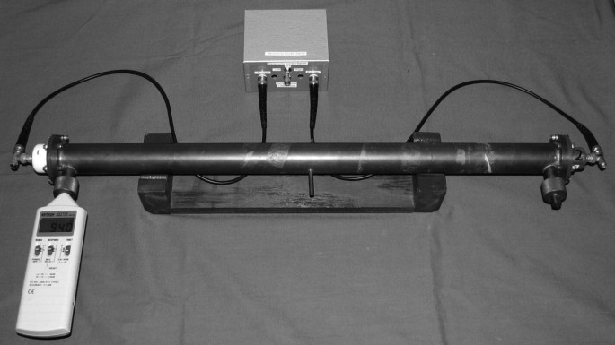
A standing wave resonator used for reciprocity calibration is capped at each end with the small, reversible, electrodynamic transducers shown in Fig. 10.26. Two ½ inch (1.27 cm) compression fittings are located very close to the ends of the resonator. An Extech™ Model 407736, Type-2 sound level meter is placed in one fitting, and the other is plugged with a solid rod. The small tube at the center allows gases other than air to be used as the calibration medium. At the top of the photo is a custom switch box that allows the swept-sine signal produced by a dynamic signal analyzer to be routed to either reversible transducer #1 or #2 after it has been passed through a precision 1.000 ohm current-sensing resistor
Fig. 10.26 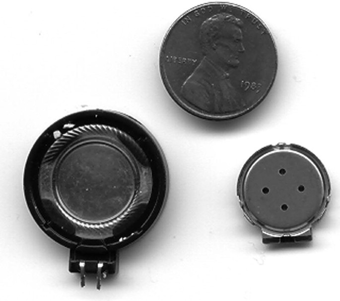
The two small reversible electrodynamic transducers that are used for the reciprocity calibration. The US penny is shown as a size comparison. Each reversible transducer is mounted on a plate that matches the flanges at the ends of the waveguide. The free-cone resonance frequency of the larger transducer is about 2.8 kHz, and that of the smaller one is about 1.7 kHz. Each transducer is mounted on a flange that attaches to the end of the resonator shown in Fig. 10.25
-
(a)


Notes
- 1.
Prof. Polack was on the faculty at the Danish Technical University (less than a 10 min drive from Lyngby to the Brüel & Kjær Headquarters in Nærum, Denmark) when he made this design. He is currently a professor at Université Pierre et Marie Curie and the Head of Doctoral School of Mechanics, Acoustics, Electronics and Robotics (SMAER, ED 391).
- 2.
The resultant resonator was conical. It can be modeled easily in DeltaEC as a single CONE element (plus an electrodynamic driver VESPEAKER at one end and an OPNBRANCH radiation condition at the other end). This is a lot easier than 28 lumped elements once you accept that a cone will solve the problem.
- 3.
Some say thermodynamics is the field where every partial derivative has its own name.
- 4.
We assume that ρm is independent of x throughout most of this book. Many thermoacoustic phenomena, including engines and refrigerators, rely on the x dependence of Tm and ρm, so the fundamental equations of thermoacoustics are more complicated [8].
- 5.
Analog Devices, Inc. sells a wonderful temperature sensing integrated circuit (AD 592) that sources one microampere of current for each degree of absolute temperature, making electronic temperature compensation nearly trivial.
- 6.
In acoustics, the equivalent of “optical trapping” is acoustical levitation superstability (see Sect. 15.4.7): M. Barmatz and S. L. Garrett, “Stabilization and oscillation of an acoustically levitated object,” US Pat. No. 4,773,266 (Sept. 27, 1988).
- 7.
In my estimation, one of the most significant engineering breakthroughs of the twentieth century was the invention, by Harold S. Black (1989–1983) at Bell Labs, of the negative feedback amplifier in 1928. In Black’s own words, “Our patent application was treated in the same manner as one for a perpetual-motion machine. In a climate where more gain was better, the concept that one would throw away gain to improve stability, bandwidth, etc., was inconceivable before that time.”
- 8.
The “true” definition of a root-mean-squared (rms) amplitude is always tied to the power associated with that amplitude. To account for non-sinusoidal waveforms, engineers introduce a dimensionless “crest factor,” CF, that is defined as the ratio of the peak value of a waveform to its rms value. For a sine waveform, CF (sine) =\( \sqrt{2} \), for a triangular waveform, CF (triangle) =\( \sqrt{3} \), and for a half-wave rectified sinewave, CF (half-wave rectified) = 2. Most instruments that claim to measure the “true rms” value of a parameter (e.g., voltage) will exhibit an accuracy that decreases with increasing crest factor. For measurement of Gaussian noise, instruments that tolerate 3 < CF < 5 are usually adequate.
- 9.
The weighting of A, B, C, and D (no weighting) levels are specified in several international standards, for example, the International Standards Organization (ISO) 3746:2010, and are plotted in Fig. 10.6.
- 10.
The transfer function for sound pressure at the eardrum to the sound pressure presented to the outer ear is above 14 dB of gain from 2.5 to 3.2 kHz as shown in Table 2 of the ANSI-ASA S3.4 Standard.
- 11.
When we include thermoviscous dissipation on the walls of the tube, the velocity will not be constant throughout the tube’s cross-section, since the no-slip boundary condition for a viscous fluid requires that the longitudinal velocity vanish at the tube’s walls. In many cases, the ratio of the viscous penetration depth, δν, to the tube’s radius, a, is small, δν ≪ a, so the flow velocity is nearly uniform throughout most of the tube’s cross-section. The thermal effects near the wall increase the compressibility of the gas (see Sect. 9.3.2), so they also create a small velocity perpendicular to the wall.
- 12.
For simplicity, we can assume that the source and microphone are both located at the same end of the resonator. If they were at opposite ends, then their relative phase would shift by 180° degrees in going from an odd to an even mode of the resonator.
- 13.
The reciprocity principle also applies in vector form. If we applied a vector force at some location, ①, on a flexible structure, and the vector displacement is measured at some other location, ②, we would observe the same vector displacement at ① if the same vector force were applied at ②.
- 14.
The primary calibration of voltage is simpler (in principle, although it requires temperatures near absolute zero for the Josephson junction) since it is possible to relate the dc voltage across a superconducting Josephson junction to the resulting oscillation frequency, f, since their ratio is determined by Planck’s constant, h, and the charge on an electron, e: V ≡ nhf /2e, where n is an integer. 2e/h = (483.5978) MHz/μV.
- 15.
This is equivalent to saying that the transducers are non-compliant in much the same way that the “constant displacement drive” for a string does not “feel” the load of the string and preserves the “fixed” boundary condition. For reciprocity calibration of transducers that behave as an ultracompliant driver (i.e., a constant force drive equivalent), see [43].
- 16.
The acoustic center of a reversible microphone or a sound source under free-field conditions is defined as the extrapolated center of the spherically diverging wave field (see Problem 4 in Chap. 12).
- 17.
Within the cone, the pressure amplitudes would be larger than those of a spherically spreading wave if the source’s volume velocity was the same in both cases. If the cone subtends a solid angle, Ω, then the pressures would be enhanced by a factor of 4π/Ω, assuming the additional load would not reduce the source’s volume velocity.
- 18.
If β 2 is negative, then there is a family of sinusoidal horn shapes (e.g., a globe terminated in a cusp) that describe the shape of the bell of the flute commonly associated with Indian snake charmers or the English horn, first used in the by Rossini, in 1829, in the opera, William Tell. [See B. N. Nagarkar and R. D. Finch, “Sinusoidal horns,” J. Acoust. Soc. Am. 50(1) 23–31 (1971).]
- 19.
A nonuniform power transmission coefficient does not necessarily reduce the value of guided-wave enhancement of the coupling to an electrodynamic transducer, since human perception of low-frequency musical content is not particularly sensitive to such a nonuniform response. The best example of such a psycho-acoustic tolerance may be the success of the Bose Wave™ radio that employs a long serpentine duct that is driven by the rear of the forward-radiating speakers as shown in US Pat. No. 6,278,789 (Aug. 21, 2001).
- 20.
Fritz Haber was also one of the world’s most infamous chemists, having developed the gas that was used to murder prisoners in the Nazi death camps.
References
M.J. Lighthill, Waves in Fluids (Cambridge University Press, 1978). See §2.6; ISBN 0 521 29233 6 (paperback)
V.A. Del Grosso, New equation for the speed of sound in natural waters (with comparisons to other equations). J. Acoust. Soc. Am. 56(4), 1084–1091 (1974)
A.J. Zuckerwar, D.S. Mazel, Sound Speed Measurements in Liquid Oxygen-Liquid Nitrogen Mixtures, NASA Technical Paper 2464 (NASA Langley Research Center, Hampton, 1985)
M.R. Moldover, R.M. Gavioso, J.B. Mehl, L. Pitre, M. de Podesta, J.T. Zhang, Acoustic gas thermometry. Metrologia 51, R1–R19 (2014)
M.R. Moldover et al., Measurement of the universal gas constant ℜ using a spherical acoustic resonator. J. Res. Nat. Bur. Stand. 93, 85–144 (1988)
E. Polturak, S.L. Garrett, S.G. Lipson, Precision acoustic gas analyzer for binary mixtures. Rev. Sci. Inst. 57(11), 2837–2841 (1986)
G.W. Swift, Thermoacoustics: A Unifying Perspective for Some Engines and Refrigerators, 2nd edn. (ASA Press/Springer, 2017). See Eq. (2.74), pg. 50; ISBN 978–3–319-66932-8
F.W. Giacobbe, Estimation of Prandtl numbers in binary mixtures of helium and other noble gases. J. Acoust. Soc. Am. 96(6), 3568–3680 (1994)
G.S.K. Wong, Speed of sound in standard air. J. Acoust. Soc. Am. 79(5), 1359–1366 (1986)
M. Greenspan, Comments on ‘Speed of sound in standard air’. J. Acoust. Soc. Am. 82(1), 370–372 (1987)
Stanford Research Systems Model BGA244, Binary Gas Analyzer, www.thinkSRS.com
S. Garrett, Sonic gas analyzer for hydrogen and methane. Proc. Acoustics 08, Paris, 29 June–4 July, 2008, pp. 2767–2772
S.L. Garrett, G.W. Swift, R.E. Packard, Helium gas purity monitor for recovery systems. Physica 107B, 601–602 (1981)
M.V. Golden, R.M. Keolian, S.L. Garrett, Sonic gas analyzers, in Proc. 16th Int. Congress on Acoustics and 135th Meeting Acoust. Soc. Am., vol. III, (Seattle, WA, 20–26 June 1998), pp. 1705–1706
G.M. Sessler, J.E. West, Electret transducers: A review. J. Acoust. Soc. Am. 53(6), 1589–1600 (1973)
National Semiconductor Model LM2907
J.N. Tjøtta, S. Tjøtta, Nonlinear equations of acoustics, in Frontiers of Nonlinear Acoustics: Proc. 12th International Symposium on Nonlinear Acoustics, ed. by M. F. Hamilton, D. T. Blackstock, (Elsevier Scientific Publishers, Ltd, London, 1990)
L.D. Landau, E.M. Lifshitz, Fluid Mechanics, 2nd edn. (Butterworth-Heinemann, 1987). §81; ISBN 0 7506 2767 0
F.M.F. Chapman, Decibels, SI units, and standards. J. Acoust. Soc. Am 108(2), 480 (2000)
H. Fletcher, W.A. Munson, Loudness, its definition, measurement, and calculation. J. Acoust. Soc. Am. 5(2), 82–108 (1933)
D.W. Robinson, R.S. Dadson, A re-determination of the equal-loudness relations for pure tones. Br J. Appl. Phys. 7, 166–188 (1956)
ISO 226, Acoustics – Normal Equal-Loudness Contours (International Standards Organization, Geneva, 2003)
B.R. Glasberg, B.C.J. Moore, Prediction of absolute thresholds and equal loudness contours using a modified loudness model. J. Acoust. Soc. Am. 120(2), 585–588 (2006)
American National Standard for Sound Level Meters, ANSI-ASA S1.4-1983, most recently reaffirmed by the American National Standards Institute (ANSI), 21 Mar 2006
S. Fidell, A review of US aircraft noise regulatory policy. Acoustics Today 11(4), 26–34 (2015)
P.D. Schomer, Criteria for assessment of noise annoyance. Noise Control Eng. J. 53(4), 132–144 (2005)
American National Standard Method for the Calculation of the Speech Intelligibility Index, ANSI-ASA S3.5-1997
G.W. Swift, Thermoacoustic engines. J. Acoust. Soc. Am. 84(4), 1145–1180 (1988). See Eq. (59)
W.R. MacLean, Absolute measurement of sound without a primary standard. J. Acoust. Soc. Am. 12(1), 140–146 (1940)
J. W. Strutt (Lord Rayleigh), Proc. London Math. Soc. 4, 357 (1983); Scientific Papers, Vol. I, (Dover, 1964), pp. 140. Note: The Scientific Papers are available from the Acoustical Society of America in a fully-searchable version on CD-ROM
R.K. Cook, Absolute pressure calibrations of microphones. J. Res. Natl. Bur. Stand. 25, 489 (1940) and J. Acoust. Soc. Am. 12(1), 415–420 (1941)
G.S.K. Wong, T. F. W. Embleton (eds.), AIP Handbook of Condenser Microphones (Am. Inst. Phys., 1995). Chapters 8–12; ISBN 1-56396-284-5
R.J. Bobber, Underwater Electroacoustic Measurements (Naval Research Laboratory, Underwater Sound Reference Division (U.S. Govt. Printing Office), 1970). See §2.3
L.L. Foldy, H. Primakoff, A general theory of passive linear electroacoustic transducers and the electroacoustic reciprocity theorem. I. J. Acoust. Soc. Am. 17(2), 109–120 (1945). Also H. Primakoff and L. L. Foldy “A general theory of passive linear electroacoustic transducers and the electroacoustic reciprocity theorem. II,” J. Acoust. Soc. Am. 19(1), 50–58 (1947)
R.M. Keolian, personal communication
R.P. Feynman, R.B. Leighton, M. Sands, The Feynman Lectures on Physics, vol II (Addison-Wesley, 1964). See §37–1
F.V. Hunt, Symmetry in the equations for electromechanical coupling. J. Acoust. Soc. Am. 22(5), 672 (1950)
F.V. Hunt, Electroacoustics: The Analysis of Transduction and Its Historical Background (Harvard, 1954). See “Symmetry and Equivalent Circuits” and “The Burdens of Antisymmetry,” pp. 105–116
L.E. Kinsler, A.R. Frey, A.B. Coppens, J.V. Sanders, Fundamentals of Acoustics, 4th edn. (Wiley, 2000). See Ch. 14.4(b), “Antireciprocal Transducers”; ISBN 0–471–84789-5
I. Rudnick, Unconventional reciprocity calibration of transducers. J. Acoust. Soc. Am. 63(3), 1923–1925 (1978)
S.L. Garrett, S. Adams, S. Putterman, I. Rudnick, Resonant nonlinear mode conversion in He II. Phys. Rev. Lett. 41(6), 413–416 (1978)
G.W. Swift, S.L. Garrett, Resonance reciprocity calibration of an ultracompliant transducer. J. Acoust. Soc. Am. 81(5), 1619–1623 (1987)
R.J. Bobber, Underwater Electroacoustic Measurements (Naval Research Laboratory, Underwater Sound Reference Division (U.S. Govt. Printing Office), 1970)
G.S.K. Wong, Primary pressure calibration by reciprocity, in AIP Handbook of Condenser Microphones, ed. by G. S. K. Wong, T. F. W. Embleton, (1995). Am. Inst. Phys.; ISBN 1-56396-284-5
V. Nedzelintsky, Primary method for calibrating free-field response, in AIP Handbook of Condenser Microphones, ed. by G.S.K. Wong, T.F.W. Embleton, (1995). Am. Inst. Phys; ISBN 1-56396-284-5
I. Rudnick, M.N. Stein, Reciprocity free field calibration of microphones to 100 Kc in air. J. Acoust. Soc. Am. 20(6), 818–825 (1948)
S. Barrera-Figueroa, Free-field reciprocity calibration of measurement microphones at frequencies to 150 kHz. J. Acoust. Soc. Am. 144(4), 2572–2583 (2018)
E. Frederiksen, J.I. Christensen, Pressure reciprocity calibration – instrumentation, results, and uncertainty. Brüel & Kjær Tech. Rev. 1, 5–26 (1998)
H.E. Bass, J. Bhattacharyya, M.A. Garcés, M. Hedlin, J.V. Olsen, R.L. Woodward, Infrasound. Acoustics Today 2(1), 9–19 (2006)
T.B. Gabrielson, Reciprocity calibration for infrasound sensors. J. Acoust. Soc. Am. 141(5), 3568 (2017)
L.E. Kinsler, A.R. Frey, A.B. Coppens, J.V. Sanders, Fundamentals of Acoustics, 4th edn. (Wiley, 2000). See Eq. (10.5.4); ISBN 0-471-84789-5
R.S. Wakeland, Use of electrodynamic drivers in thermoacoustic refrigerators. J. Acoust. Soc. Am. 107(2), 827–832 (2000)
M.A.G. Timmer, K. de Blok, T.H. van der Meer, Review on the conversion of thermoacoustic power into electricity. J. Acoust. Soc. Am. 143(2), 841–857 (2018)
Morel Acoustics USA, Inc., Brookline, MA
W.C. Ward, Cost-effective electrodynamic drivers with improved efficiency for thermoacoustic refrigerators. J. Acoust. Soc. Am. 100(4), 2847 (1996)
M. Fitzpatrick, Electrodynamic driver for the Space Thermoacoustic Refrigerator (STAR), M.S. thesis, Physics Department, Naval Postgraduate School, Monterey, CA, 1988; DTIC report no. ADA 192337, p. 80
S.L. Garrett, J.A. Adeff, T.J. Hofler, Thermoacoustic refrigerator for space applications. AIAA J. Thermophys. Heat Trans. 7(4), 595–599 (1993)
S.L. Garrett, High power thermoacoustic refrigerator. US Pat. No. 5,647,216 (15 July 1997)
J. Liu, S. Garrett, Characterization of a small moving-magnet electrodynamic linear motor for use in a thermoacoustic refrigerator. J. Acoust. Soc. Am. 118(4), 2289–2295 (2005)
G.A. Yarr, J.C. Corey, Linear electrodynamic machine. US Pat. No. 5,389,844 (14 Feb. 1995)
C.H. Allen, I. Rudnick, A powerful high frequency siren. J. Acoust. Soc. Am. 19(5), 857–865 (1947)
W.L. Nyborg, Acoustic streaming, in Physical Acoustics, ed. by W. P. Mason, vol. IIB, (Academic, 1964)
J.K. Hilliard, Historical review of horns used for audience-type sound reproduction. J. Acoust. Soc. Am. 59(1), 1–8 (1976)
P.M. Morse, Vibration and Sound, 2nd edn. (McGraw-Hill, 1948). Reprinted by the Acoust. Soc. Am., 1995. See Fig. 58; ISBN 0-88318-876-7
V. Salmon, Generalized plane wave horn theory. J. Acoust. Soc. Am. 17(3), 199–211 (1946). and “A new family of horns,” J. Acoust. Soc. Am. 17(3), 212–218 (1946)
I. Rudnick, On the attenuation of high amplitude waves of stable saw-tooth form propagating in horns. J. Acoust. Soc. Am. 30(4), 339–342 (1948)
P. Bèquin, C.L. Morfey, Weak nonlinear propagation of sound in a finite exponential horn. J. Acoust. Soc. Am. 109(6), 2649–2659 (2001)
L.L. Beranek, Acoustics. Acoust. Soc. Am. (1996). Chapter 9; ISBN 0-88318-494-X
M. Kleiner, Electroacoustics (Taylor & Francis, 2013). Chapter 19; ISBN 978-1-4398-3618-70
H. Witschi, Profiles in toxicology, Fritz Haber: 1868–1934. Toxicol. Sci. 55, 1–2 (2000)
P.W. Mullen, Modern Gas Analysis (Interscience, 1955)
L.L. Beranek, Acoustic Measurements (Wiley, 1949), pp. 161–171
A.E. Aliev et al., Underwater sound generation using carbon nanotube projectors. Nano Letters (Am. Chem. Soc.) 10, 2374–2380 (2010)
Author information
Authors and Affiliations
Rights and permissions
Open Access This chapter is licensed under the terms of the Creative Commons Attribution 4.0 International License (http://creativecommons.org/licenses/by/4.0/), which permits use, sharing, adaptation, distribution and reproduction in any medium or format, as long as you give appropriate credit to the original author(s) and the source, provide a link to the Creative Commons license and indicate if changes were made.
The images or other third party material in this chapter are included in the chapter's Creative Commons license, unless indicated otherwise in a credit line to the material. If material is not included in the chapter's Creative Commons license and your intended use is not permitted by statutory regulation or exceeds the permitted use, you will need to obtain permission directly from the copyright holder.
Copyright information
© 2020 The Author(s)
About this chapter

Cite this chapter
Garrett, S.L. (2020). One-Dimensional Propagation. In: Understanding Acoustics. Graduate Texts in Physics. Springer, Cham. https://doi.org/10.1007/978-3-030-44787-8_10
Download citation
DOI: https://doi.org/10.1007/978-3-030-44787-8_10
Published:
Publisher Name: Springer, Cham
Print ISBN: 978-3-030-44786-1
Online ISBN: 978-3-030-44787-8
eBook Packages: Physics and AstronomyPhysics and Astronomy (R0)