Comfort for the Computationally Crippled

Abstract

The difference between engineering and science, and all other human activity, is the fact that engineers and scientists make quantitative predictions about measurable outcomes and can specify their uncertainty in such predictions. Because those predictions are quantitative, they must employ mathematics. This chapter is intended as review of some of the more useful mathematical concepts, strategies, and techniques that are employed in the description of vibrational and acoustical systems and in the calculation of their behavior. Topics in this review include techniques such as Taylor series expansions, integration by parts, and logarithmic differentiation. Equilibrium and stability considerations lead to relations between potential energies and forces. The concept of linearity leads to superposition and Fourier analysis. Complex numbers and phasors are introduced along with the techniques for their algebraic manipulation. The discussion of physical units is extended to include their use for predicting functional dependencies of resonance frequencies, quality factors, propagation speeds, flow noise, and other system behaviors using similitude and the Buckingham Π-theorem to form dimensionless variables. Linearized least-squares fitting is introduced as a method for extraction of experimental parameters and their uncertainties and error propagation is presented to allow those uncertainties to be combined.

“The discussion of any problem in science or engineering has two aspects: the physical side, the statement of the facts of the case in everyday language and of the results in a manner that can be checked by experiment; and the mathematical side, the working out of the intermediate steps by means of the symbolized logic of calculus. These two aspects are equally important and are used side by side in every problem, one checking the other.” [1]

The difference between engineering and science, and all other human activity, is the fact that engineers and scientists make quantitative predictions about measurable outcomes and can specify their uncertainty in such predictions. Because those predictions are quantitative, they must employ mathematics. This chapter is intended as an introduction to some of the more useful mathematical concepts, strategies, and techniques that are employed in the description of vibrational and acoustical systems and the calculations of their behavior.

It is not necessary to master the content of this chapter before working through this textbook. Other chapters will refer back to specific sections of this chapter as needed. If you are unsure of your competence or confidence with mathematics, it may be valuable to read through this chapter before going on.

1.1 The Five Most Useful Math Techniques

Below is a list of the five most useful mathematical techniques for the study of acoustics and vibration based on my experience. Techniques number one and number five are self-explanatory. The other three will be introduced in more detail in this section.

• Substitution

• Taylor series

• The product rule or integration by parts

• Logarithmic differentiation

• Garrett’s First Law of Geometry: “Angles that look alike are alike.”

1.1.1 Taylor Series

Acoustics and vibration are the “sciences of the subtle.” Most of our attention will be focused on small deviations from a state of stable equilibrium. For example, a sound pressure level¹ of 115 dB_SPL is capable of creating permanent damage to your hearing with less than 15 min of exposure per day [2]. That acoustic pressure level corresponds to a peak excess pressure of p₁ = 16 Pa (1 Pa = 1 N/m²). Since “standard” atmospheric pressure is p_m = 101,325 Pa [3], that level corresponds to a relative deviation from equilibrium that is less than 160 parts per million (ppm) or p₁/p_m = 0.016%.

If we assume that any parameter of interest (e.g., temperature, density, pressure) varies smoothly in time and space, we can approximate the parameter’s value at a point (in space or time) if we know the parameter’s value at some nearby point (typically, the state of stable equilibrium) and the value of its derivatives evaluated at that point.² The previous statement obscures the true value of the Taylor series because it is frequently used to permit substitution of the value of the derivative, as we will see throughout this textbook.

Let us start by examining the graph of some arbitrary real function of position, f(x), shown in Fig. 1.1. At position x_o, the function has a value, f(x_o). At some nearby position, x_o + dx, the function will have some other value, f(x_o + dx), where we will claim that dx is a small distance without yet specifying what we mean by “small.”

Fig. 1.1

Graph of an arbitrary function of position, f(x). The straight dashed line is tangent to f(x) at x_o. It represents the first derivative (slope) of f(x) evaluated at x_o

The value of f(x_o + dx) can be approximated if we know the first derivative of f(x) evaluated at x_o.

$$ f\left({x}_o+ dx\right)\cong f\left({x}_o\right)+{\left.\frac{df}{dx}\right|}_{x_o} dx $$

(1.1)

As can be seen in Fig. 1.1, the approximation of Eq. (1.1) produces a value that is slightly less than the actual value f(x_o + dx) in this example. That is because the actual function has some curvature that happens to be upward in this case. The differential, dx, is used to represent both finite and infinitesimal quantities, depending upon context. For approximations, dx is assumed to be small but finite. For derivation of differential equations, it is assumed to be infinitesimal.

We can improve the approximation by adding another term to the Taylor series expansion of f(x) that includes a correction proportional to the second derivative of f(x), also evaluated at x_o. For the example in Fig. 1.1, the curvature is upward so the second derivative of f(x), evaluated at x_o, is a positive number, so ${\left({d}^2f/{dx}^2\right)}_{x_o}>0$.

If the curve had bent downward, the second derivative would have been negative. A more accurate approximation than Eq. (1.1) is provided by the following expression containing a correction proportional to (dx)²:

$$ f\left({x}_o+ dx\right)\cong f\left({x}_o\right)+{\left.\frac{df}{dx}\right|}_{x_o} dx+{\left.\frac{d^2f}{dx^2}\right|}_{x_o}\frac{(dx)^2}{2} $$

(1.2)

Since (dx)² is intrinsically positive and the upward curvature makes d²f/dx² positive, we can see that this second-order correction improves our estimate of f(x_o + dx). Had the curvature been downward, making ${\left({d}^2f/{dx}^2\right)}_{x_o}<0$, then the second-order correction would have placed the estimated value of f(x_o + dx) the first-order (linear) estimate, as required, since (dx)² would still be positive.

In principle, we can continue to improve the Taylor series approximation by adding higher and higher-order derivatives, although it is rare to extend such a series extended beyond the first three terms in Eq. (1.2). The full generic form of the Taylor series is provided in Eq. (1.3).

$$ f\left({x}_o+ dx\right)=f\left({x}_o\right)+\sum \limits_{n=1}^{\infty }{\left.\frac{f^n(x)}{(dx)^n}\right|}_{x_o}\frac{(dx)^n}{n!}=f\left({x}_o\right)+\sum \limits_{n=1}^{\infty }{f}^{(n)}\left({x}_o\right)\frac{{\left(x-{x}_o\right)}^n}{n!} $$

(1.3)

The Taylor series approach of Eq. (1.3) can be used to express continuous functions in a power series. Below are some functions that have been expanded about x_o = 0. As we will see, they will be particularly useful when |x| ≪ 1.

$$ {e}^x=1+x+\frac{x^2}{2!}+\frac{x^3}{3!}+\cdots =1+x+\frac{x^2}{2}+\frac{x^3}{6}+\cdots $$

(1.4)

$$ \sin (x)=x-\frac{x^3}{3!}+\frac{x^5}{5!}-\cdots =x-\frac{x^3}{6}+\frac{x^5}{120}-\cdots $$

(1.5)

$$ \cos (x)=1-\frac{x^2}{2!}+\frac{x^4}{4!}-\cdots =1-\frac{x^2}{2}+\frac{x^4}{24}-\cdots $$

(1.6)

$$ \tan (x)=x+\frac{x^3}{3}+\frac{2{x}^5}{15}+\frac{17{x}^7}{315}+\frac{62{x}^9}{2835}\cdots $$

(1.7)

$$ \ln \left(1+x\right)=x-\frac{x^2}{2}+\frac{x^3}{3}-\frac{x^4}{4}+\cdots $$

(1.8)

$$ {\left(1+x\right)}^{\alpha }=1+\alpha x+\frac{\alpha \left(\alpha -1\right)}{2!}{x}^2+\frac{\alpha \left(\alpha -1\right)\left(\alpha -2\right)}{3!}{x}^3+\cdots $$

(1.9)

1.1.2 The Product Rule or Integration by Parts

If we have two functions of x, say u(x) and v(x), the product rule tells us how we can take the derivative of the product of those functions.

$$ \frac{d(uv)}{dx}=\frac{du}{dx}v+u\frac{dv}{dx} $$

(1.10)

This rule can be extended, for example, to the product of three functions of a single variable, where we have now added w(x).

$$ \frac{d(uvw)}{dx}=\frac{du}{dx} vw+u\frac{dv}{dx}w+ uv\frac{dw}{dx} $$

(1.11)

Although it is not the intent of this chapter to derive all the quoted results, it is instructive, in this context, to introduce the concept of a differential.³ If we say that a small change in x, by the amount dx, produces a small change in u(x), by the amount du, and that |du/u| ≪ 1, then we can show that Eq. (1.10) is correct by taking the product of the small changes.

$$ d(uv)=\left(u+ du\right)\left(v+ dv\right)- uv=u(dv)+v(du)+(du)(dv) $$

(1.12)

Since both du and dv are small, the product of du times dv must be much less than u (dv) or v (du). If we make the changes small enough, then (du) (dv) can be neglected in Eq. (1.12). Throughout this textbook, we will make similar assumptions regarding our ability to ignore the products of two very small quantities [4].

The Fundamental Theorem of Calculus states that integration and differentiation are inverse processes. By rearranging Eq. (1.10) and integrating each term with respect to x, we can write an expression that allows for integration of the product of one function and the derivative of another function.

$$ \int u(x)\frac{dv}{dx} dx=u(x)v(x)-\int v\frac{du}{dx} dx $$

(1.13)

This result is known as the method of integration by parts.

1.1.3 Logarithmic Differentiation

The natural logarithm can be defined in terms of the integral of x⁻¹.

$$ \int \frac{dx}{x}=\ln (x)+C $$

(1.14)

C is a constant. If we again apply the Fundamental Theorem of Calculus, we can write an expression for the differential, dx, in terms of the derivative of ln (x), remembering that the derivative of any constant must vanish.

$$ d\left(\ln x\right)=\frac{dx}{x} $$

(1.15)

We will frequently be confronted by mathematical expressions that contain products and exponents. We can simplify our manipulations of such terms by taking the natural logarithms of those expressions and then differentiating. One typical example is the determination of the temperature change, dT, that accompanies a pressure change, dp, in a sound wave propagating under adiabatic conditions based on the Ideal Gas Law in Eq. (1.16) and the Adiabatic Gas Law in Eq. (1.17).

$$ pV=n\mathrm{\Re}T $$

(1.16)

$$ {pV}^{\gamma }=\mathrm{constant} $$

(1.17)

If we substitute the Ideal Gas Law into the Adiabatic Gas Law, we can write the absolute (kelvin) temperature, T, and pressure, p, in terms of a constant, C, related to the initial pressure and volume; the universal gas constant, ℜ; and the polytropic coefficient, γ. (Do not worry if none of this is familiar at this point, it is only meant to illustrate the mathematics and will be treated explicitly in Sect. 7.1.4.)

$$ {pV}^{\gamma }={\left( n\mathit{\Re T}\right)}^{\gamma }{p}^{1-\gamma}\kern1em \Rightarrow \kern1em {T}^{\gamma }{p}^{1-\gamma }=\frac{p_o{V}_o^{\gamma }}{{\left( n\mathit{\Re}\right)}^{\gamma }}\equiv C $$

(1.18)

Again, C is just a constant that depends upon the initial conditions. The natural logarithm of both sides of the right-hand version of Eq. (1.18) produces Eq. (1.19).

$$ \gamma \ln T+\left(1-\gamma \right)\ln p=\ln C $$

(1.19)

Using logarithmic differentiation, as expressed in Eq. (1.15),

$$ \gamma \frac{dT}{T}+\left(1-\gamma \right)\frac{dp}{p}=0\kern1em \Rightarrow \kern1em \frac{dT}{T}=\frac{\left(\gamma -1\right)}{\gamma}\frac{dp}{p} $$

(1.20)

Rearranging terms and recalling that we substituted into the Adiabatic Gas Law, this result provides an expression for the change in the temperature of an ideal gas in terms of the change in the pressure due to a sound wave that is propagating under adiabatic conditions.

$$ {\left(\frac{\partial T}{\partial p}\right)}_s=\frac{\left(\gamma -1\right)}{\gamma}\frac{T}{p} $$

(1.21)

The subscript “s” has been placed along the partial derivative to remind us that the change in temperature with pressure is evaluated for an adiabatic process in which the specific entropy (per unit mass), s, is held constant. As will be illustrated in our investigations of the coupling between sound waves and temperature changes, this is a particularly useful result. It has only been previewed here to illustrate how simple it is to do some calculations by taking a logarithm of an expression before differentiation. This will also be a rather convenient approach for calculation of the uncertainty of a result based on the uncertainty in the parameters that were used to calculate the result (i.e., “error propagation”; see Sect.1.8.4).

1.2 Equilibrium, Stability, and Hooke’s Law

Pause for a moment as you are reading and look around. Close your eyes, count to ten, and then open your eyes. Probably not much has changed. This is because most of the material we observe visually is in a state of stable equilibrium.⁴ For an object to be in equilibrium, the vector sum of all the forces acting on that body (i.e., the net force) must be zero, and the first derivative of the object’s potential energy with respect to its position must be zero. For that equilibrium state to be stable, the second derivative of the object’s potential energy must be positive.

Figure 1.2 illustrates three possible equilibrium conditions based on the rate of change of a body’s potential energy with position. For this illustration, let us assume that the solid curve represents the height, z, above some reference height, z_o, in a uniform gravitational field. The (gravitational) potential energy, PE (z), of each of the three balls shown in Fig. 1.2 is therefore proportional to their height, z, where the mass of each ball is m and g is the acceleration due to gravity that is assumed to be independent of z: PE (z) = mg (z–z_o).

Fig. 1.2

Potential energy (proportional to height) is shown as a function of position for three objects that are at rest in an equilibrium state within a gravitational field. The ball at the left is in a state of neutral equilibrium, since it can move to the left or the right by a small distance and not change its potential energy. The ball at the center is in a state of unstable equilibrium. Although the net force (gravitational downward and the force of the surface upward) is zero, if it is displaced by an infinitesimal distance to either the right or the left, it will leave its equilibrium position. The ball at the right is in a position of stable equilibrium. If it is displaced by an infinitesimal distance to either the right or to the left, the net force on the ball will tend to return it toward its equilibrium position. The dashed line is a parabola that is fit to match the curvature of the line near the position of stable equilibrium corresponding to the quadratic contribution in the Taylor series expansion of Eq. (1.23)

The three balls in Fig. 1.2 each respond to a small displacement from their equilibrium positions differently. We can think of the solid curve as representing a flat surface on the left, two peaks at the center and the right, and a valley between two peaks. All three balls are in a state of mechanical equilibrium because the vector sum of the force of gravity (down) and of the surface (up) is zero. In all three cases, the first derivative of the potential energy vanishes at all three locations: d(PE)/dx = 0. The ball on the left is in a state of neutral equilibrium because it can be moved to the left or to the right by a small distance and it will still be at equilibrium, even at its displaced position. The curve at that location is flat and horizontal.

The other two balls are located at local extrema. The slopes of the tangents to the curves at those extrema are just both as horizontal and as the flat region on the left.⁵ The ball near the center of Fig. 1.2 is at the top of the “hill,” so d(PE)/dx = 0 and d²(PE)/dx² < 0. The ball near the right in that figure is at the lowest point in the valley, so d(PE)/dx = 0, but down in the valley, d²(PE)/dx² > 0.

The ball at the top of the peak is in a state of unstable equilibrium because if it is displaced by an infinitesimal amount in either direction, it will run away from its equilibrium position. In general, objects in states of unstable equilibrium do not remain in those states for very long.

The ball at the lowest point in the valley is in a state of stable equilibrium. If it is displaced in either direction, the potential energy increases, and the ball can reduce its energy by returning to its position of stable equilibrium. A dashed parabola has been drawn which matches the second derivative of the actual potential energy curve. The greater the distance from the point of stable equilibrium, the greater the difference between the actual curve representing the potential energy and the dashed parabola, but for small displacements from equilibrium, the real potential energy curve and the dashed parabola will be indistinguishable. The dashed parabola represents the second-order term in a Taylor series expansion of the potential energy about the equilibrium position provided in Eq. (1.23).

With this understanding of equilibrium and stability, we are in a position to formalize the application of potentials and forces to develop the formalism that is used to characterize the oscillations of systems that obey Hooke’s law.

1.2.1 Potentials and Forces

The relationship between forces and potential energy can be extended beyond our simple stability example. In general, the net (vector) force, ${\overrightarrow{F}}_{net}$, is the negative of the gradient of the (scalar) potential energy: $\overrightarrow{\nabla}(PE)=-{\overrightarrow{F}}_{net}$.⁶ This is consistent with the definitions of work and energy.

$$ {W}_{1,2}\equiv {\int}_1^2\overrightarrow{F}\bullet d\overrightarrow{x}={(PE)}_1-{(PE)}_2=-\Delta (PE) $$

(1.22)

The right-hand side assumes that $\overrightarrow{F}$ is a conservative force⁷ and the work, W_1,2, done in moving an object from position 1 to position 2, over some distance along the direction of the force (indicated by the “dot product” under the integral), leads to a change in potential energy, −Δ(PE). Again, application of the Fundamental Theorem of Calculus leads to the desired relationship between the gradients of the potential energy and the net force: $\overrightarrow{\nabla}(PE)=-{\overrightarrow{F}}_{net}$.

If we limit ourselves to the current example of a ball in the valley, we can expand the potential energy about the stable equilibrium position that is identified as x_o.

$$ PE\left({x}_o+ dx\right)= PE\left({x}_o\right)+{\left.\frac{d^2(PE)}{dx^2}\right|}_{x_o}\frac{(dx)^2}{2}+{\left.\frac{d^3(PE)}{dx^3}\right|}_{x_o}\frac{(dx)^3}{6}+\dots $$

(1.23)

Note that the first derivative of PE is missing from Eq. (1.23) because it is zero if x_o is the equilibrium position.⁸ The term proportional to (dx)³ corresponds to the contribution to the difference between the actual curve and the dashed parabola in Fig. 1.2. If the deviation between the two curves is symmetric, then the leading correction term would be proportional to (dx)⁴. If the deviation is not symmetric, the leading correction term will be proportional to (dx)³.

In our one-dimensional example, the gradient of the potential energy will simply be the derivative of Eq. (1.23) with respect to x.

$$ {F}_{net}(dx)=-\frac{d(PE)}{dx}=-{\left.\frac{d^2(PE)}{dx^2}\right|}_{x_o}(dx)-{\left.\frac{d^3(PE)}{dx^3}\right|}_{x_o}\frac{(dx)^2}{2}-\cdots $$

(1.24)

For sufficiently small displacements from equilibrium, the parabolic approximation to the potential energy curve (i.e., the dashed parabola in Fig. 1.2) provides an adequate representation, and therefore the series of Eq. (1.24) that describes the force can be truncated after the first term.

$$ {F}_{net}(dx)\cong -{\left.\frac{d^2(PE)}{dx^2}\right|}_{x_o}(dx)\equiv -\mathrm{K}(dx) $$

(1.25)

The result in Eq. (1.25) is known as Hooke’s law. ⁹ It states that the net force is proportional to the displacement from equilibrium, dx. Because of the minus sign, the net force is directed opposite to that displacement if Κ > 0. The new constant, Κ, is known as the “stiffness” when the potential energy is created by the extension or compression of a spring. It is equal to the negative of the second derivative of the potential energy, evaluated at the equilibrium position, x_o.

In this form, it is obvious that a positive curvature in the potential energy (i.e., d²(PE)/dx² > 0) leads to a stable equilibrium but that a negative curvature in the potential energy causes the system to become unstable. In an unstable state of equilibrium, a small displacement from equilibrium creates a force that causes a small displacement to grow, regardless of the sign of the original displacement; at a position of unstable equilibrium, the stiffness constant, Κ, is a negative number.

The approximation represented by Hooke’s law leads to a linear relationship between net force on a body and the displacement of that body from its position of stable equilibrium. It is normally introduced in elementary mechanics courses as the law which describes the force exerted by a spring when the spring is displaced from its equilibrium length, x_o. Two such springs are showed schematically in Fig. 1.3.

Fig. 1.3

Schematic representation of two springs that obey Hooke’s law for small displacements from their equilibrium positions, x_o. The spring at the left represents a coil of wire with one end fixed (represented by the hatched wall) at x = 0 and an equilibrium length of x_o. The spring at the right represents an air-filled cylinder that is closed at the end located at x = 0 and is sealed at the opposite end by a close-fitting, frictionless piston. (It is possible to purchase a piston and cylinder combination that behaves very much like this leak-tight, frictionless idealization. It is called an Airpot^® and consists of a glass cylinder and a matched graphite piston: www.airpot.com. One such Airpot^® is shown in Prob. 4 at the end of Chap. 7, in Fig. 7.6.) The equilibrium position of the gas spring at x_o occurs when the mean gas pressure inside the cylinder is equal to the mean gas pressure outside the cylinder

Both of the springs in Fig. 1.3 obey Hooke’s law if the displacements, dx, from the equilibrium position at x_o are small: (dx)/x_o ≪ 1. In both cases, large displacements from equilibrium will lead to nonlinear behavior. For the coil spring, excess compression will cause the coils to close up, and the force necessary for further compression will be much larger than predicted by Hooke’s law. Similarly, for excess extension, the coils will straighten out, again requiring excess force, until the material fractures and the broken end can be moved an infinite distance without requiring any additional force. Similar deviations from the linear behavior predicted by Hooke’s law occur for the gas spring. Two examples of the force vs. displacement that go beyond the linear regime are illustrated in Fig. 1.4.

Fig. 1.4

Two graphs of force vs. displacement which illustrate deviations from linear Hooke’s law behavior for two systems that each possess a position of stable equilibrium. At the left is a graph representing springs like those shown in Fig. 1.3. For small displacements from the equilibrium position, x_o, the force is a linear function of displacement. As x becomes significantly smaller than x_o, the spring “stiffens,” producing significantly larger forces for a given displacement, presumably because adjacent coils have made contact. As x becomes significantly greater than x_o, the spring again stiffens. In this limit, the coils have begun to uncoil, and the force is increasing due to the tensile strength of the coil spring’s material. Eventually, the material fractures or the piston is removed from the cylinder, and the force goes to zero. The graph at the right might represent the restoring force of a pendulum that is displaced from its equilibrium vertical position hanging down at θ_o = 0 (see Fig. 1.5). Again, there is a linear portion of the force vs. angular displacement for small values of θ ⪡ 1, but as the angle increases, less force is required for each increment of angle. This nonlinear spring behavior is called “softening”

1.2.2 A Simple Pendulum

To emphasize the fact that “linear” behavior is not restricted to linear motion, consider the spherical mass suspended from a rigid ceiling by a (massless) string of length, L, in a uniform gravitational field, as shown schematically in Fig. 1.5. Its position of stable equilibrium corresponds to the mass hanging vertically downward beneath the point of suspension; hence θ_o = 0. In this case, the gravitational potential energy is a function of the angular displacement corresponding to the change in vertical height of the sphere’s center of mass, h(θ), within a gravitational field that is presumed to produce a constant gravitational acceleration, g. The relationship between the displacement angle, θ, and the height change, h(θ ), can be calculated from trigonometry.

$$ PE\left(\theta \right)= mgL\left[1-\cos \theta \right]\cong mgL\left[\frac{\theta^2}{2}-\frac{\theta^4}{24}+\cdots \right] $$

(1.26)

Fig. 1.5

The pendulum consists of a sphere of mass, m, which is supported by a massless string. The distance from the point of support to the center of mass of the sphere is L. When the sphere is displaced from its equilibrium position, θ_ο = 0, this angular displacement, θ, causes the sphere’s center of mass to rise above its equilibrium height by a vertical distance, h. The associated increase in the gravitational potential energy of the sphere is given by Eq. (1.26). The restoring torque on the pendulum is given by the gradient in the potential energy and is shown schematically in the graph of Fig. 1.4 (right)

The above approximation uses a power (Taylor) series expansion of the cosine function from Eq. (1.6). The magnitude of the corresponding restoring torque, N(θ ), is given by the negative of the gradient of the potential energy with respect to angle.

$$ N\left(\theta \right)=-\frac{\partial \left[ PE\left(\theta \right)\right]}{\partial \theta}\cong - mgL\left[\theta -\frac{\theta^3}{6}+\cdots \right] $$

(1.27)

For θ ≪ 1, the restoring torque is proportional to the angular displacement from stable equilibrium. In this limit, this results in a torsional stiffness that is a constant. For larger displacements from equilibrium, additional effects generated by the θ³ term in Eq. (1.27) reduce the torque producing the “softening” behavior shown in Fig. 1.4 (Right).

1.3 The Concept of Linearity

At least 95% (by weight?) of the systems analyzed in this textbook will assume that the dynamical processes occur within the linear regime. This assumption brings with it amazing mathematical and physical simplifications. As will be discussed here, linearity guarantees that:

• 1. The frequency of oscillation of a “free” system is amplitude-independent (isochronism).

• 2. The steady-state response of a driven linear system occurs only at the driving frequency.

• 3. We can superimpose an infinite number of responses to simple stimuli to determine the linear system’s response to a very complicated stimulus and vice versa.

The founder of modern science, Galileo Galilei (1564–1642), was the first to record his observation that the period of a pendulum was independent of the amplitude of its displacement. Legend has it that he made that observation in the Cathedral of Pisa when he was a student living in that city. Being bored in church, he noticed that when the wind moved the chandeliers, the period of oscillation, measured against his own pulse rate, was independent of the amplitude of chandeliers’ swing. Although Galileo recognized the value of this amplitude independence for time-keeping devices, it was not until 17 years after Galileo’s death that the great Dutch physicist, Christiaan Huygens (1629–1695), described his “pendulum clock” and other time pieces with errors of less than 1 min/day (later, less than 10 s/day) whose accuracy relied on the amplitude independence of the period of the pendulum.

The behavior of nonlinear springs is dramatically different than the Hooke’s law behavior [5]. When driven at a frequency, ω, the system can respond at multiples, or sub-multiples of the driving frequency [6], and can produce non-zero time-averaged changes in the equilibrium position. Nonlinear elastic behavior in solids is responsible for the fact that the thermal expansion coefficient of solids is non-zero. As temperature increases, the thermal vibrational amplitude of the solid’s atoms causes their equilibrium separation to change [7].

Although we have thus far only considered the behavior of systems displaced a small distance from their position of stable equilibrium (thus producing a linear restoring force), we will combine that result with the behavior of masses and dampers in the next chapter on simple harmonic oscillators. The dynamics of masses and dampers also exhibit a substantial linear regime. Newton’s Second Law of Motion, $\overrightarrow{F}=m\ddot{\overrightarrow{x}}$, is linear because it relates the acceleration of a mass to the net force acting on that mass. Acceleration is the second time derivative of displacement and does not involve higher powers of displacement. Similarly, there is a regime where the damping force can be linear in velocity, $v(t)=\dot{x}(t)\equiv dx(t)/ dt$, which is the first time derivative of displacement. Although we will investigate the behavior of the damped simple harmonic oscillator in the next chapter, we can write down the equation for a linear operator, L (x), that describes the response of such an oscillator to an externally applied time-dependent force, F (t).

$$ \underline{L}(x)=m\frac{d^2x}{dt^2}+{R}_m\frac{dx}{dt}+\mathrm{K}x=F(t) $$

(1.28)

To simplify our discussion of linear response, we can lump all of these linear operations performed on x into a general linear operator, L(x), where L is underlined to remind us that it is an “operator,” not a function.¹⁰ That operator defines a combination of mathematical procedures that are applied to an independent variable, x in this case. The operator in Eq. (1.28) is a second-order linear differential equation with constant coefficients, those coefficients being the mass, m; the mechanical resistance, R_m; and the stiffness, Κ.

By substitution into Eq. (1.28), it is easy to demonstrate that all linear operations exhibit both an additive and a multiplicative property where a is an arbitrary scalar.

$$ \underset{\_}{L}\left(x+y\right)=\underset{\_}{L}(x)+\underset{\_}{L}(y) $$

(1.29)

$$ \underset{\_}{L}(ax)=a\underset{\_}{L}(x) $$

(1.30)

In fact, these two properties of linear operators can be extended indefinitely.

$$ \underset{\_}{L}\left( ax+ by+ cz+\cdots \right)=a\underset{\_}{L}(x)+b\underset{\_}{L}(y)+c\underset{\_}{L}(z)+\cdots $$

(1.31)

These properties demonstrate that if we have a solution to Eq. (1.28), that any scalar multiple of that solution is also a solution; if we double the force, we double the response. Similarly, if both x_a(t) and x_b(t) are two responses to two forces, F_a(t) and F_b(t), possibly acting at two different frequencies, then their sum is the response to the sum of those forces.

$$ \underset{\_}{L}\left({x}_a+{x}_b\right)=\underset{\_}{L}\left({x}_a\right)+\underset{\_}{L}\left({x}_b\right)={F}_a(t)+{F}_b(t) $$

(1.32)

1.4 Superposition and Fourier Synthesis

“Superposition is our compensation for enduring the limitations of linearity”. [8]

The ability exhibited by Eq. (1.31) to combine solutions to linear equations is so significant that it has its own name: The Principle of Superposition. It guarantees that if we can decompose a complicated excitation into the sum of simpler excitations, we can calculate the responses to the simple excitations, and then we can combine those simple solutions to determine the response to the more complicated excitation.

We all have experience with this concept when we locate a point on a two-dimensional surface using Cartesian coordinates. The x and y axes form an orthogonal basis that specifies the horizontal and vertical directions. When we want to specify a particular point on that surface, we draw a vector, $\overrightarrow{r}$, from the origin of the coordinate system to the point and project that vector on to our orthogonal axes by taking the dot product of the vector, $\overrightarrow{r}$, with the unit vectors, ${\hat{e}}_x$ and ${\hat{e}}_y$, along each axis.

$$ \left(x,y\right)=\left(\overrightarrow{r}\bullet {\hat{e}}_x,\overrightarrow{r}\bullet {\hat{e}}_y\right) $$

(1.33)

In that way, the ordered sequence of two numbers, (x, y), produced by those two operations, uniquely specifies a point on the plane.

This simple concept can be extended to a representation of a function as a superposition of orthogonal functions. A general n^th-order, linear differential equation with constant coefficients, a_i, will have the form expressed below:

$$ {a}_n\frac{d^nx}{dt^n}+{a}_{n-1}\frac{d^{n-1}x}{dt^{n-1}}+\cdots +{a}_1\frac{dx}{dt}+{a}_o=F(t) $$

(1.34)

There will be n linearly independent solutions to such an equation, where we mean that the solutions are “independent” if it is not possible to express one of the linearly independent solutions in terms of linear combinations of the others.¹¹ With a few minor exceptions (such as flexural waves on bars and plates), our focus in this textbook will be on systems described by second-order differential equations with constant coefficients. For that case n = 2, so there will be two linearly independent solutions. One convenient choice of independent solutions for vibration and acoustics is the sine and cosine functions.

The representation of periodic functions as the sum of simple oscillating functions dates back to the third century BC when ancient astronomers proposed models of planetary motion based on epicycles. The first use of trigonometric functions as a basis for solving a linear differential equation was made by Jean-Baptiste Joseph Fourier (1768–1830). In his Treatise on the Propagation of Heat in Solid Bodies, published in 1807, he used the technique that now bears his name to analyze the diffusion of heat through a metal plate.

As we will see, the solutions to equations describing vibration and sound are particularly simple if the disturbances are sinusoidal in space and/or time. For more complicated disturbances, which are periodic with period, T₁, it is possible to decompose the disturbance into the sum of sinusoidal disturbances with the same period as the complicated waveform. If the complicated waveform is a continuous function, the periodic waveform can be represented by an infinite number of sines and cosines, each with the correct amplitude, that have frequencies that are integer multiples of the fundamental frequency of the complicated waveform, ${f}_1={T}_1^{-1}=\omega /2\pi .$

$$ f(t)=\frac{A_o}{2}+\sum \limits_{n=1}^{\infty}\left[{A}_n\cos \left( n\omega t\right)+{B}_n\sin \left( n\omega t\right)\right]. $$

(1.35)

The coefficients, A_n and B_n, are determined in the same way we selected the x and y coordinates for a point on a Cartesian plane; we take the equivalent of the dot product of the complicated function with the linearly independent basis functions over an entire period, T. Such a “dot product,” also known as the “inner product,” is represented by the following integrals:

$$ {A}_0=\frac{1}{T}{\int}_0^Tf(t)\kern0.5em dt\kern0.5em \mathrm{and}\kern0.5em {A}_n=\frac{2}{T}{\int}_0^Tf(t)\cos \left( n\omega t\right) dt\kern0.5em \mathrm{for}\kern0.5em n\ge 1 $$

(1.36)

$$ {B}_n=\frac{2}{T}{\int}_0^Tf(t)\sin \left( n\omega t\right) dt $$

(1.37)

Since sin (0) = 0, there is no need for B_o. Since cos (0) = 1, A_o is just the average of f(t) over one period,¹² divided by the period, T. The sine and cosine functions are linearly independent, and the orthogonality of the harmonics of the individual sine and cosine functions can be expressed in terms of the Kronecker delta function, δ_m,n, which is zero if m ≠ n and one if m = n.

$$ {\displaystyle \begin{array}{l}\frac{2}{T}{\int}_0^T\cos \left( m\omega t\right)\cos \left( n\omega t\right) dt={\delta}_{m,n}\\ {}\frac{2}{T}{\int}_0^T\sin \left( m\omega t\right)\sin \left( n\omega t\right) dt={\delta}_{m,n}\end{array}} $$

(1.38)

Depending upon the nature of f(t), it is possible that many of the A_n and B_n coefficients may be zero. If f(t) is symmetric about the time axis, then A_o = 0. If f(t) = f(−t), then f(t) is an even function of t and B_n = 0 for all n, since sine is an odd function. Similarly, if f(t) = −f(−t), then f(t) is an odd function of t, and A_n = 0 for all n, since cosine is an even function.

The process of assembling a “complex” waveform from simpler sinusoidal components is known as Fourier synthesis. To illustrate Fourier synthesis, let us represent a square wave, f_square(t), of unit amplitude and period, T, that is defined for one period below and is shown in Fig. 1.6:

$$ {f}_{\mathrm{square}}(t)=\left\{\begin{array}{cc}+1& 0\le t<T/2\\ {}-1& T/2\le t<T\end{array}\right. $$

(1.39)

Fig. 1.6

The square wave defined in Eq. (1.39) is shown along with the sum of the first through fourth non-zero Fourier components. The first term is simply a sinusoidal waveform that is synchronized with the square wave. The third harmonic contribution starts to deform the sum into a shape that more closely resembles the square wave. Addition of the fifth harmonic, and then the seventh harmonic, improves the fidelity of the superposition and makes the slope of the zero-crossing transitions more nearly vertical. Clearly superposition of an infinite number of harmonics would be required to simulate the infinite slope of those transitions and reduce the “ripple” on the plateaus, although the small (9%) overshoot will remain. It does not disappear as more terms are added; it simply becomes narrower [10]. Since the square wave is not a “continuous” function but has a discontinuous slope, its Fourier series representation will have an “overshoot” (known as “ringing”) about those transitions. This is known as the “Gibbs phenomenon”

Since f_square (t) is symmetric, A_o = 0 and because it is an odd function of t, only the B_n coefficients will be non-zero. Substitution of Eq. (1.39) into Eq. (1.37) breaks the integral into two parts.

$$ {B}_n=\frac{2}{T}\left[{\int}_0^{T/2}\sin \left( n\omega t\right) dt-{\int}_{T/2}^T\sin \left( n\omega t\right) dt\right] $$

(1.40)

The integral of the sin (ax) over x is available from any table of integrals. My favorite is the Russian compilation by Gradshteyn and Ryzhik [9].

$$ \int \sin (ax)\; dx=\frac{-1}{a}\cos (ax)+C $$

(1.41)

For this problem ω = 2π/T, so a = 2πn/T.

$$ {B}_n=\frac{1}{n\pi}\left[-\cos {\left.\left(\frac{2\pi nt}{T}\right)\right|}_0^{T/2}+\cos {\left.\left(\frac{2\pi nt}{T}\right)\right|}_{T/2}^T\right] $$

(1.42)

For odd values of n, B_n = (4/nπ), and for even values of n, B_n = 0, so the Fourier series representation of our unit symmetric square wave can be written as an infinite sum.

$$ {f}_{\mathrm{square}}(t)=\frac{4}{\pi}\left[\sin \left(\frac{2\pi t}{T}\right)+\frac{1}{3}\sin \left(\frac{6\pi t}{T}\right)+\frac{1}{5}\sin \left(\frac{10\pi t}{T}\right)+\cdots \right] $$

(1.43)

Again, the fact that ω = 2π/T allows us to rewrite this result in terms of angular frequencies.

$$ {f}_{\mathrm{square}}(t)=\frac{4}{\pi}\left[\sin \left(\omega\;t\right)+\frac{\sin \left(3\omega\;t\right)}{3}+\frac{\sin \left(5\omega\;t\right)}{5}+\cdots \right] $$

(1.44)

The sum of the first four terms is shown in Fig. 1.6, illustrating that the addition of successive terms makes the Fourier series superposition an ever more faithful representation of f_square (t).¹³

We could repeat the process to determine the Fourier representation of a triangle wave f_triangle (t), but if we simply recognize that a triangular wave is the integral of a square wave, then we can integrate Eq. (1.44) term by term.

$$ {f}_{\mathrm{triangle}}(t)=\frac{4}{\pi^2}\left[\cos \left(\omega\;t\right)+\frac{\cos \left(3\omega\;t\right)}{9}+\frac{\cos \left(5\omega\;t\right)}{25}+\dots \right] $$

(1.45)

Since the shape of the triangle wave is much closer to that of a sine or cosine, the high-frequency components decay more quickly (as n⁻²) than those of the square wave (as n⁻¹).

1.5 Convenience (Complex) Numbers

“The most beautiful formula in mathematics: e ^jπ + 1 = 0.” [11]

Calculus is a set of rules that allow us to convert expressions that involve integrals and derivatives into algebraic equations. The simplest of these rules are those which allow us to write down the integrals and derivatives of polynomials and exponentials:

$$ \frac{d\left({ax}^n\right)}{dx}={anx}^{n-1}\kern0.5em ;\kern1.5em \int {ax}^n dx=\frac{ax^{n+1}}{n+1}+C $$

(1.46)

$$ \frac{d\left({ae}^{bx}\right)}{dx}={abe}^{bx}\kern0.5em ;\kern1.5em \int {ae}^{bx} dx=\frac{ae^{bx}}{b}+C $$

(1.47)

We have already exploited the simplicity of Eq. (1.46) because our Taylor series expansions resulted in polynomial representations of various functions (see Sect. 1.1.1). In this section, we will exploit the simplicity of Eq. (1.47) in a way that allows us to encode the two linearly independent solutions to a second-order differential equation into a single function by simply multiplying one of those two solutions by the square root of (−1). That special linear coefficient will be designated as $j\equiv \sqrt{-1}$.

The fact that j allows us to combine (i.e., superimpose) the solutions to differential equations of interest in a way that permits the use of Eq. (1.47) to do our calculus is the reason I call j the “convenience number.” Unfortunately, I am the only person who calls j the convenience number. Everyone else calls j the unit “imaginary number.”¹⁴ Numbers that contain an imaginary component are called “complex numbers.” This poor historical choice of nomenclature suggests that there is something “complex” about the use of j when the contrary is true; j makes computations simpler.

To appreciate the convenience of j, we can start by examining the solution to the simplest homogeneous second-order differential equation with a constant coefficient that has been designated ${\omega}_o^2$ for reasons that will become obvious in the next chapter.

$$ \frac{d^2x}{dt^2}+{\omega}_o^2x=0\kern2em \mathrm{or}\kern2em \frac{d^2x}{dt^2}=-{\omega}_o^2x $$

(1.48)

When written as the right-hand version of Eq. (1.48), it is clear that we seek a solution which produces the negative of itself when differentiated twice. Sine and cosine functions have exactly that property, being linearly independent.¹⁵

$$ \frac{d\sin (at)}{dt}=a\cos (at)\kern0.5em ;\kern1em \int \sin (at) dt=-\frac{\cos (at)}{a}+C $$

(1.49)

$$ \frac{d\cos (at)}{dt}=-a\sin (at)\kern0.5em ;\kern1.5em \int \cos (at) dt=\frac{\sin (at)}{a}+C $$

(1.50)

Double differentiation of either sine or cosine regenerates the negative of the original function, as required by Eq. (1.48).¹⁶ Superposition allows us to write the complete solution to Eq. (1.48) by introducing two arbitrary scalar constants, A and B:

$$ x(t)=A\cos \left({\omega}_ot\right)+B\sin \left({\omega}_ot\right) $$

(1.51)

Using our definition of $j\equiv \sqrt{-1}$ and the rules for differentiating exponentials in Eq. (1.47), we see that an exponential with an imaginary exponent will also obviously satisfy Eq. (1.48), where again A and B are scalar constants that facilitate superposition of the two solutions.

$$ x(t)={Ae}^{j{\omega}_ot}+{Be}^{-j{\omega}_ot} $$

(1.52)

Thanks to our earlier investment in the Taylor series expansions of sine, cosine, and exponential functions, we see that these solutions are identical if we use Eq. (1.4) to expand e^jθ in a power series and group together terms that are multiplied by j.

$$ {e}^{j\theta}=1-\frac{\theta^2}{2!}+\frac{\theta^4}{4!}-\cdots +j\left[\theta -\frac{\theta^3}{3!}+\frac{\theta^5}{5!}-\cdots \right]=\cos \theta +j\sin \theta $$

(1.53)

This result is known as Euler’s formula named after Swiss mathematician and physicist Leonhard Euler (1707–1783). By similar means, we see that e^-jθ = cos θ – j sin θ. It is also easy to demonstrate the relationship between exponential functions of imaginary arguments and trigonometric functions by taking sums and differences of these expressions of Euler’s identity.

$$ \cos \theta =\frac{e^{j\theta}+{e}^{- j\theta}}{2}\kern0.5em ;\kern1.5em \sin \theta =\frac{e^{j\theta}-{e}^{- j\theta}}{2j} $$

(1.54)

These algebraic manipulations certainly build confidence in the equivalence of the two solutions of Eq. (1.48), but for our purposes, a geometric interpretation will have significant utility in our study of both vibrations and waves.

1.5.1 Geometrical Interpretation on the Argand Plane

To develop and exploit this geometric interpretation of exponential functions, which contain complex numbers within their arguments (hereafter referred to as complex exponentials), we can represent a complex number on a two-dimensional plane known as the “complex plane” or the Argand plane. In that representation, we define the x axis as the “real axis” and the y axis as the “imaginary axis.” This is shown in Fig. 1.7. In this geometric interpretation, multiplication by j would correspond to making a “left turn” [12], that is, making a 90° rotation in the counterclockwise direction. Since j∗j = j² = −1 would correspond to two left turns, a vector pointing along the real axis would be headed backward, which is the equivalent of multiplication by −1.

Fig. 1.7

Representation of a complex number, z, on the Argand plane. The projection of z on the Cartesian x axis represents the real part of z, and the y axis projection represents the imaginary part of z. The projections of the vector, $\overrightarrow{r}$, onto the real and imaginary axes provide ℜe(z) = x = |$\overrightarrow{r}$| cos θ and ℑm(z) = y = |$\overrightarrow{r}$| sin θ. The ordinary rules of plane geometry and trigonometry apply. For example, |$\overrightarrow{r}$| = (x² + y²)^½ and θ = tan⁻¹(y/x)

In this textbook, complex numbers will be expressed using bold font. A complex number, z = x + jy, where x and y are real numbers, would be represented by a vector of length, $\left|\overrightarrow{r}\right|=\sqrt{x^2+{y}^2}$, from the origin to the point, z, on the Argand plane, making an angle with the positive real axis of θ = tan⁻¹(y/x). The complex number could also be represented in polar coordinates on the Argand plane as z = Ae ^jθ, where A = $\mid \overrightarrow{r}\mid$. The geometric and algebraic representations can be summarized by the following equation:

$$ \mathbf{z}=x+ jy=\left|\mathbf{z}\right|\left(\cos \theta +j\sin \theta \right)=\left|\mathbf{z}\right|{e}^{j\theta} $$

(1.55)

1.5.2 Phasor Notation

In this textbook, much of our analysis will be focused on response of a system to a single-frequency stimulus. We will use complex exponentials to represent time-harmonic behavior by letting the angle θ increase linearly with time, θ = ω_ot + ϕ, where ω_o is the frequency (angular velocity) which relates the angle to time and ϕ is a constant that will accommodate the incorporation of initial conditions (see Sect. 2.1.1) or the phase between the driving stimulus and the system’s response (see Sect. 2.5). As the angle, θ, increases with time, the projection of the uniformly rotating vector, $\overrightarrow{x}=\mid \overrightarrow{x}\mid {e}^{j{\omega}_ot+ j\phi t}\equiv \hat{\mathbf{x}}{e}^{j{\omega}_ot}$, traces out a sinusoidal time dependence on either axis. This choice is also known as phasor notation. In this case, the phasor is designated $\hat{\mathbf{x}}$, where the “hat” reminds us that it is a phasor and its representation in bold font reminds us that the phasor is a complex number.

$$ \hat{\mathbf{x}}=\left|\hat{\mathbf{x}}\right|{e}^{j\theta} $$

(1.56)

Although the projection on either the real or imaginary axis generates the time-harmonic behavior, the traditional choice is to let the real component (i.e., the projection on the real axis) represents the physical behavior of the system. For example, $x(t)\equiv \mathit{\Re e}\left[\hat{\mathbf{x}}{e}^{j{\omega}_ot}\right]$.

1.5.3 Algebraic Operations with Complex Numbers

The rectangular representation and the polar representation have complementary utility, as the following review of algebraic operations will demonstrate. Addition and subtraction of two complex numbers allow a vector operation to be converted to an algebraic operation, as it would if our concern were analytic geometry instead of complex arithmetic. Starting with two complex vectors, ${\mathbf{A}}_{\mathbf{1}}={a}_1+{jb}_1=\mid {\mathbf{A}}_{\mathbf{1}}\mid {e}^{j{\theta}_1}\kern0.5em \mathrm{and}\kern0.5em {\mathbf{A}}_{\mathbf{2}}={a}_2+{jb}_2=\mid {\mathbf{A}}_{\mathbf{2}}\mid {e}^{j{\theta}_2}$, where a and b are real scalars, their sum and difference are just the sums and differences of their real and imaginary components:

$$ {\mathbf{A}}_{\mathbf{1}}+{\mathbf{A}}_{\mathbf{2}}=\left({a}_1+{a}_2\right)+j\left({b}_1+{b}_2\right)\kern0.5em \mathrm{and}\kern0.5em {\mathbf{A}}_{\mathbf{1}}-{\mathbf{A}}_{\mathbf{2}}=\left({a}_1-{a}_2\right)+j\left({b}_1-{b}_2\right) $$

(1.57)

The utility of the polar representation becomes manifest for operations involving multiplication and division. In terms of their real and imaginary components, a and b, multiplication of two complex numbers proceeds just as in the case of the multiplication of two binomials.

$$ {\mathbf{A}}_{\mathbf{1}}{\mathbf{A}}_{\mathbf{2}}=\left({a}_1+{jb}_1\right)\left({a}_2+{jb}_2\right)=\left({a}_1{a}_2-{b}_1{b}_2\right)+j\left({a}_1{b}_2+{b}_1{a}_2\right) $$

(1.58)

Multiplication by anything other than a scalar is not a linear process, so the real and imaginary components become mixed by multiplication. The equivalent operation expressed in polar coordinates is both simpler to execute and easier to visualize.

$$ {\mathbf{A}}_{\mathbf{1}}{\mathbf{A}}_{\mathbf{2}}=\mid {\mathbf{A}}_{\mathbf{1}}\mid {e}^{j{\theta}_1}\mid {\mathbf{A}}_{\mathbf{2}}\mid {e}^{j{\theta}_2}=\mid {\mathbf{A}}_{\mathbf{1}}\Big\Vert {\mathbf{A}}_{\mathbf{2}}\mid {e}^{j\left({\theta}_1+{\theta}_2\right)} $$

(1.59)

The division of two complex numbers in component form introduces the procedure known as rationalization. This is accomplished by multiplying both the numerator and denominator by the complex conjugate of the denominator. The complex conjugate of a complex number is just that number with the sign of the imaginary part changed. The complex conjugate is usually designated by an asterisk: z∗ = x – jy; hence, ℑm[(z)(z∗)] = ℑm[(z∗)(z)] = 0 (see Sect. 1.5.5). When faced with division by a complex number, the rationalization process makes the denominator a real number and allows the result to be separated into its real and imaginary components.

$$ \frac{{\mathbf{A}}_{\mathbf{1}}}{{\mathbf{A}}_{\mathbf{2}}}=\frac{\left({a}_1+{jb}_1\right)}{\left({a}_2+{jb}_2\right)}=\frac{\left({a}_1+{jb}_1\right)}{\left({a}_2+{jb}_2\right)}\frac{\left({a}_2-{jb}_2\right)}{\left({a}_2-{jb}_2\right)}=\frac{\left({a}_1{a}_2+{b}_1{b}_2\right)}{a_2^2+{b}_2^2}+j\frac{b_1{a}_2-{a}_1{b}_2}{a_2^2+{b}_2^2} $$

(1.60)

Again, the process of division is nonlinear, so the real and imaginary components are comingled. The polar representation provides both greater insight and simplified execution.

$$ \frac{{\mathbf{A}}_{\mathbf{1}}}{{\mathbf{A}}_{\mathbf{2}}}=\frac{\left|{\mathbf{A}}_{\mathbf{1}}\right|{e}^{j{\theta}_1}}{\left|{\mathbf{A}}_{\mathbf{2}}\right|{e}^{j{\theta}_2}}=\frac{\left|{\mathbf{A}}_{\mathbf{1}}\right|}{\left|{\mathbf{A}}_{\mathbf{2}}\right|}{e}^{j\left({\theta}_1-{\theta}_2\right)}\kern1em \mathrm{if}\kern1em \left|{\mathbf{A}}_{\mathbf{2}}\right|\ne 0 $$

(1.61)

Raising a number to a real power or extracting a real root is also simplified using a polar representation.

$$ {\mathbf{A}}^n={\left(\left|\mathbf{A}\right|{e}^{j\theta}\right)}^n={\left|\mathbf{A}\right|}^n{e}^{j n\theta} $$

(1.62)

Since the extraction of the n^th root generates n solutions, it is helpful to include the periodicity of the complex exponential explicitly, since addition of integer multiples of 2π to the angle θ does not change its value.

$$ \sqrt[n]{\mathbf{A}}={\mathbf{A}}^{\left(1/n\right)}={\left(\mathbf{A}{e}^{j\left(\theta +2\pi \nu \right)}\right)}^{\left(1/n\right)}={\left|\mathbf{A}\right|}^{\left(1/n\right)}{e}^{j\left[\left(\theta /n\right)+2\pi \left(\nu /n\right)\right]} $$

(1.63)

This will generate n roots with ν = 0, 1, 2, …, (n – 1). Inclusion of larger integer values of ν ≥ n just regenerates the same roots. For example, if we calculate the square root of 4,

$$ \sqrt{4}=2{e}^{j\left(0/2\right)}=2\kern1.5em \mathrm{and}\kern1.5em \sqrt{4}=2{e}^{j\left(2\pi /2\right)}=2{e}^{j\pi}=-2. $$

(1.64)

The cube root of 8 has three solutions:

$$ {\displaystyle \begin{array}{l}\sqrt[3]{8}=2{e}^{j\left(0/3\right)}=2{e}^{j0}=2\\ {}\sqrt[3]{8}=2{e}^{j\left(2\pi /3\right)}=2\left[\cos \left(2\pi /3\right)+j\sin \left(2\pi /3\right)\right]=-1+j\sqrt{3}\\ {}\sqrt[3]{8}=2{e}^{j\left(4\pi /3\right)}=2\left[\cos \left(4\pi /3\right)+j\sin \left(4\pi /3\right)\right]=-1-j\sqrt{3}\end{array}} $$

(1.65)

In polar representation, the three roots are three two-unit-long vectors separated by 120°, with the first of those three solutions aligned along the real axis.

The calculation of the natural logarithm of a complex number is also simplified by the use of the polar form.¹⁷

$$ \ln \left[\mathbf{A}\right]=\ln \left[\left|\mathbf{A}\right|{e}^{j\theta}\right]=\ln \left[\left|\mathbf{A}\right|\right]+ j\theta $$

(1.66)

As for the usual case with real numbers,log₁₀[A] = (log₁₀e) ln [|A|e^jθ] ≅ 0.4343 ln [A].

1.5.4 Integration and Differentiation of Complex Exponentials

The primary motivation for the introduction of complex exponentials is the ease with which it is possible to write their integrals or derivatives as was expressed in Eq. (1.47).

1.5.5 Time Averages of Complex Products (Power)

Two complex numbers are said to be complex conjugates if the imaginary parts are negatives of each other.

$$ \mathrm{If}\kern0.5em \mathbf{A}=a+ jb=\left|\mathbf{A}\right|{\mathrm{e}}^{j\theta},\kern0.5em \mathrm{then}\kern0.5em \mathbf{A}\ast =a- j b=\left|\mathbf{A}\right|{e}^{- j\theta} $$

(1.67)

The polar version shows that the complex conjugate, A∗, of a complex number, A, is just the reflection of A about the real axis. The complex conjugate provides a direct method for calculation of the modulus |A| of a complex number as well as for the extraction of the real and imaginary parts of a complex number..

$$ \left|\mathbf{A}\right|\equiv \sqrt{{\mathbf{AA}}^{\ast}}={\left[\left(a+ jb\right)\left(a- jb\right)\right]}^{1/2}={\left({a}^2+{b}^2\right)}^{1/2} $$

(1.68)

$$ \mathit{\Re e}\left[\mathbf{A}\right]=\left(\frac{1}{2}\right)\left(\mathbf{A}+{\mathbf{A}}^{\ast}\right)=\left(\frac{1}{2}\right)\left[\left(a+ jb\right)+\left(a- jb\right)\right]=a $$

(1.69)

$$ \mathit{\Im m}\left[\mathbf{A}\right]=\left(1/2j\right)\left(\mathbf{A}-{\mathbf{A}}^{\ast}\right)=\left(1/2j\right)\left[\left(a+ jb\right)-\left(a- jb\right)\right]=b $$

(1.70)

Complex conjugates are particularly useful for the calculation of time-averaged power, 〈Π〉_t, since that calculation requires evaluation of the “dot product” between two variables that characterize a potential and a flow. For a simple harmonic oscillator, those complex variables are force, F, and velocity, v; for a fluid, they are pressure, p, and volume flow rate, U.¹⁸ The dot product guarantees that only the components of the two variables which are in-phase contribute to the result.

It is important to realize that the product of the real parts of two variables is not equal to the real part of their product.

$$ \mathit{\Re e}\left[\mathbf{F}\right]\times \mathit{\Re e}\left[\mathbf{v}\right]\ne \mathit{\Re e}\left[\mathbf{F}\mathbf{v}\right] $$

(1.71)

Using the definition of the complex conjugate in Eq. (1.67),

$$ \mathrm{\Re}e\left[\mathbf{F}\right]=\frac{1}{2}\mathrm{\Re}e\left[\mathbf{F}+{\mathbf{F}}^{\ast}\right]\kern1.5em \mathrm{and}\kern1.5em \mathrm{\Re}e\left[\mathbf{v}\right]=\frac{1}{2}\mathrm{\Re}e\left[\mathbf{v}+{\mathbf{v}}^{\ast}\right] $$

(1.72)

The instantaneous power, Π(t), can be written using the results of Eq. (1.72).

$$ {\displaystyle \begin{array}{c}\Pi (t)=F\bullet v=\frac{1}{4}\left(\mathbf{F}+{\mathbf{F}}^{\ast}\right)\left(\mathbf{v}+{\mathbf{v}}^{\ast}\right)=\frac{1}{4}\left[\left(\mathbf{F}\mathbf{v}+{\mathbf{F}}^{\ast}{\mathbf{v}}^{\ast}\right)+\left({\mathbf{F}\mathbf{v}}^{\ast}+{\mathbf{v}\mathbf{F}}^{\ast}\right)\right]\\ {}\Pi (t)=\frac{1}{2}\left(\mathit{\Re e}\left[\mathbf{Fv}\right]+\mathit{\Re e}\left[{\mathbf{F}\mathbf{v}}^{\ast}\right]\right)=\frac{1}{2}\mathit{\Re e}\left[\left|\mathbf{F}\right|\left|\mathbf{v}\right|{e}^{j\left(2\omega\;t+{\phi}_F+{\phi}_v\right)}+\left|\mathbf{F}\right|\left|\mathbf{v}\right|{e}^{j\left({\phi}_F-{\phi}_v\right)}\right]\end{array}} $$

(1.73)

The second version of the instantaneous power assumes simple harmonic time variation of both F and v at frequency, ω, with a phase difference of ϕ_F – ϕ_v. If we take the real part of the term in square brackets, the instantaneous power can be expressed in terms of two cosines.

$$ \Pi (t)=\frac{1}{2}\left|\mathbf{F}\right|\left|\mathbf{v}\right|\left[\cos \left(2\omega t+{\phi}_F+{\phi}_v\right)+\cos \left({\phi}_F-{\phi}_v\right)\right] $$

(1.74)

The time-averaged power is determined by integration of Eq. (1.74) over a complete cycle with period, T = 2π/ω, or if the integral is over a time much longer than one period. The first term is oscillatory, so the time average is zero. The second term is just a constant, so the time integral over the second term is non-zero.

$$ {\left\langle \Pi (t)\right\rangle}_t\equiv \frac{1}{T}{\int}_0^T\Pi (t) dt=\frac{1}{2}\left|\mathbf{F}\right|\left|\mathbf{v}\right|\cos \left({\phi}_F-{\phi}_v\right)=\frac{1}{2}\mathit{\Re e}\left[{\mathbf{F}}^{\ast}\mathbf{v}\right] $$

(1.75)

Taking the complex conjugate of the argument on the right-hand side of Eq. (1.75) does not change the result, since we are extracting only the real part.

$$ {\left\langle \Pi (t)\right\rangle}_t=\frac{1}{2}\mathrm{\Re}e\left[{\left({\mathbf{F}}^{\ast}\mathbf{v}\right)}^{\ast}\right]=\frac{1}{2}\mathrm{\Re}e\left[{\mathbf{v}}^{\ast}\mathbf{F}\right] $$

(1.76)

1.6 Standard (SI) Units and Dimensional Homogeneity

We take for granted that every term in any equation must have the same units as all the other terms in that same equation. This concept is known as dimensional homogeneity. From the time of Isaac Newton (1642–1727) through the early nineteenth century, mathematical theories representing physical phenomena were expressed as ratios. For example, Ohm’s law was expressed by Georg Ohm as “The force of the current in a galvanic circuit is directly as the sum of all the tensions (i.e., voltages), and inversely as the entire reduced length of the circuit.” Similarly, Hooke’s law was expressed as “Stress is proportional to strain.” The idea that laws could be written as equations with consistent units for all terms was introduced by Jean-Baptiste Joseph Fourier. He had to fight for 20 years before this radical concept gained widespread acceptance [13].

By advocating this approach, Fourier also necessarily introduced dimensional constants. At that time, his concentration was on the transfer of heat, so he introduced both the thermal conductivity, κ [W/m-K], and the convective heat transfer coefficient, h [W/m²-K].¹⁹ Not only did this make it possible to express physical laws as equations, such “constants” characterized the properties of specific materials. The American Society of Metals publishes the ASM Handbook that has 23 volumes that are filled with such constants for a variety of metals, alloys, and composites. The printed version of the ASM Handbook takes over a meter of shelf space, although it is now also available in electronic form.

Throughout this textbook, we will use the SI System of Units exclusively.²⁰ Although this system is also commonly known as “MKS” units, because it uses meter [m], kilogram [kg], and second [s], it is actually based on seven units, of which those are just the first three. The remaining “base units” that complete the system are ampere [A], kelvin [K], mole [mol], and candela [cd].²¹ These seven form the basis of other “derived” units, many of which are commonly used in acoustics and vibration: hertz, Hz [s⁻¹]; newton, N [kg-m/s²]; pascal, Pa [N/m²]; joule, J [N-m]; watt, W [J/s]; coulomb, C [A-s]; volt, V [W/A]; farad, F [C/V]; ohm, Ω[V/A]; siemens, S [Ω⁻¹]; weber, Wb [V-s]; tesla, T [Wb/m²]; and henry, H [Wb/A]. Although I was not pleased by the change of “cycles per second” to Hz and the conversion of the conductance unit from mho [℧] (the inverse of ohm) to siemens [S], this system is very convenient because it is easy to integrate mechanical and electrical effects, an important feature for acoustical transduction systems (e.g., speakers, microphones, accelerometers, geophones, seismometers, etc.).

As of the date this book is being written, only the United States, Liberia, and Burma (Myanmar) have yet to accept SI as their national standard.²² We are frequently required either to accept data that is expressed in other systems of units or to report results in other units. This textbook includes problems that require results reported in “customary units,” but it is recommended that all computations be done using SI units and then converted as required. It follows that any result that is not a pure number must be reported along with its units.

The other recommendation regarding units is that any equation should be checked to ensure dimensional homogeneity before any numerical values are placed into that equation. An equation that is dimensionally homogeneous may be wrong, but one that is not dimensionally homogeneous is meaningless. An equation that is not dimensionally homogeneous is not even wrong!

1.7 Similitude and the Buckingham Π-Theorem (Natural Units)

“I have often been impressed by the scanty attention paid even by original workers in physics to the great principle of similitude. It happens not infrequently those results in the form of ‘laws’ are put forward as novelties on the basis of elaborate experiments, which might have been predicted a priori after a few minutes of consideration.” (J. W. Strutt (Lord Rayleigh) [14])

I will be the first to admit that “a few minutes of consideration” by Lord Rayleigh might be the equivalent of many hours of my personal effort, but the idea that physical units can dictate the form of mathematical expressions describing physical laws is important at a very fundamental level. Those of you who have studied Mechanical Engineering and/or Fluid Mechanics can attest to the significance of dimensionless groups like the Reynolds number for description of viscous fluid flow and the Nusselt number for description of convective heat transfer.

Although most attention to the discussion of units focuses on the topics in the previous section and we rely on the “standard” SI System of Units to report results and execute calculations, there is an equally important role played by the use of “natural units” that is often overlooked. Because its exploitation is rather subtle, it will be introduced first by example; then it will be generalized within a more formal (and powerful) structure.

1.7.1 Three Simple Examples

The simplest vibratory system is the mass-spring oscillator. Although that topic will be covered in detail in the next chapter, there are significant results that can be obtained without even writing down the equations governing the oscillations of a mass on a spring (i.e., Newton’s Second Law of Motion and Hooke’s law). Following Fourier’s introduction of dimensional constants, we assume that the “mass” that is attached to the spring is characterized only by its mass, m. We also know that the spring is characterized by its “stiffness,” Κ, as defined in Eq. (1.25). Mass happens to be one of the SI base units. According to Eq. (1.25), the dimensions of Κ must be force divided by displacement.

$$ \left[\mathrm{K}\right]=\frac{\left[\mathrm{Force}\right]}{\left[\mathrm{displacement}\right]}=\left[\frac{N}{m}\right]=\left[\frac{kg-m}{s^2-m}\right]=\left[\frac{kg}{s^2}\right]\equiv \left[\frac{M}{T^2}\right] $$

(1.77)

For the discussions that employ dimensional analysis to extract functional relations (a part of a process called similitude), it is common to abbreviate the “base units” as M for mass, L for length or distance, T for time, and Θ for temperature.

Instead of thinking of this problem in terms of SI units, we can use m and Κ as our “natural units.” First, notice that the definitions of m and Κ involve two base units, M and T, and that both M and T appear in Κ. Let’s say we are interested in the calculation of the frequency of oscillation, f, of this simple mass-spring combination. Since frequency has the units of reciprocal time (1/T), we can ask what combination of Κ and m, the natural units for the description of this specific system, will have the units of frequency? Although it is not too difficult to simply guess the correct result, let’s employ a more formal procedure that will become useful when we analyze more complicated applications.

To express the natural frequency of vibration, f_o, in terms of Κ and m, we can let a and b be exponents and write an equation to guarantee dimensional homogeneity:

$$ {m}^a{\mathrm{K}}^b=\frac{M^a{M}^b}{T^{2b}}=\frac{1}{T}={T}^{-1}{M}^0 $$

(1.78)

The term at the far right is just included to emphasize that we are seeking a result that does not include M. Now the values of a and b can be determined by inspection: a + b = 0 so a = −b. Equating the time exponents, b = ½ so a = −½. Based solely on the units of Κ and m, we can write the required functional form of our desired result.

$$ {f}_o\propto \sqrt{\frac{\mathrm{K}}{m}} $$

(1.79)

This approach cannot determine the numerical constant that would change this proportionality into an equation. As we will see in the next chapter, if we choose to use the radian frequency, ω_ο = 2πf_o, then no numerical constant is required: ${\omega}_o=\sqrt{\mathrm{K}/m}$. If we were deriving this relationship for a more complicated system, for which an analytic solution may not exist, then an experiment or a numerical calculation could be used to determine the constant. Even more importantly, if the experiments or the numerical calculations did not obey Eq. (1.79), then there must be other parameters required to specify the dynamics, or the experiments or calculations are flawed.

What if we added damping to the mass-spring system? The damping is characterized by a mechanical resistance, R_m, that has units of [kg/s]. Now we have three parameters (m, Κ, and R_m), but those parameters still only involve two base units. When the number of parameters exceeds the number of base units, it is then possible to combine those parameters to form dimensionless groups.

Using the same approach as employed in Eq. (1.78), we can identify this dimensionless group.

$$ {m}^a{\mathrm{K}}^b{R}_m^c=\frac{M^a{M}^b{M}^c}{T^{2b}{T}^c}={M}^0{T}^0 $$

(1.80)

The resulting equations for the exponents show that a + b + c = 0 and 2b + c = 0, so c = −2b; thus a = b. These dimensionless groups are called Π-groups, based on the classic paper by Buckingham [15]. In this case, we have created one Π-group that is designated Π₁.

$$ {\Pi}_1=\frac{\mathrm{K}m}{R_m^2}=\frac{\omega_o^2{m}^2}{R_m^2}\equiv {Q}^2 $$

(1.81)

Substitution for Κ, using ω_o² = (Κ/m), produced an expression for Π₁ that will appear frequently in the next chapter as the dimensionless quality factor, Q. When damping is present, our result for frequency can only depend upon R_m through some function of Q², hence the damped frequency, ω_d = f(Κ, m, Q²). Again, that function f (Κ, m, Q²) can be determined either by experiment or by solution of the fundamental Eq. (1.28) with F(t) = 0.

One additional simple example might be helpful before introducing the general result. Equation (1.27) expresses the torque on a simple pendulum. The parameters in that expression are the mass of the bob, m; the length of the string, L; and the acceleration due to gravity, g ≌ 9.8 m/s². We have three parameters and three “base units,” so there are no dimensionless groups. As before, recognizing that frequency, either f_o or ω_o, has units of T⁻¹, the dimensional equation below can be solved for the appropriate exponents.

$$ {m}^a{L}^b{g}^c=\frac{M^a{L}^b{L}^c}{T^{2c}}=\frac{1}{T}={T}^{-1}{M}^o{L}^o $$

(1.82)

The first result is that a = 0, so the frequency is independent of the mass of the bob. Since time only enters through the acceleration due to gravity, 2c = 1 and b + c = 0, so c = −b = ½.

$$ {f}_o\propto \sqrt{\frac{g}{L}} $$

(1.83)

Even though we included the mass of the pendulum bob as a parameter, that turned out to have no effect on the pendulum’s frequency; our dimensional analysis was able to exclude that parameter from the final result even if our intuition did not.

1.7.2 Dimensionless Π-Groups

The general idea can be summarized by expressing some dependent variable, q_o, in terms of the independent variables, q₁ through q_m. Those independent variables characterize the physical process that defines the dependent variable through some function, F, of the independent variables.

$$ {q}_o=F\left({q}_1,{q}_2,\dots {q}_m\right) $$

(1.84)

q₁ through q_m define m independent parameters. If those independent parameters can be expressed with n “base units,” then there will be (m – n) dimensionless groups. If we rearrange Eq. (1.84) into a different function, G, which includes all the variables and set G equal to zero, then we obtain one more dimensionless group that results in a homogeneous expression.

For our simple oscillator examples, we solved for q_o (f_o or ω_o in our examples) based on the independent parameters. If we would have included f_o, then we would have generated one dimensionless group that would have been equal to zero. With either approach, we would have arrived at the same result.

Those three examples that dictated the functional dependence of the frequencies for three oscillators were particularly simple. We will be able to obtain these results (including the required numerical pre-factor) by solving the differential equations directly. In acoustics and vibration, there are problems for which we cannot obtain closed-form analytical solutions, even when we know the fundamental governing equations [16]. There are occasions when a numerical answer for a particular case can be obtained using digital computation, but an “answer” for a single case is not the same as a “solution.” The use of dimensional analysis can provide an independent check on an “answer” and can provide the functional form of a solution (where the “answer” might be used to produce the numerical pre-factor). Also, our dimensional solution can be used to test answers for different cases (e.g., flow velocity, object sizes, etc.), since the parameters in the numerical solution have presumably been identified.

1.7.3 Windscreen Noise*

We will complete this section by examining an acoustical example that does not easily yield to conventional mathematical analysis. Windscreens are placed around microphones to reduce the noise that such microphones detect when they measure sound in the presence of flowing air (wind). Figure 1.8 shows measurements of the sound pressure levels in one-third octave bands, ${p}_{1/3}$, as a function of the band-centered frequencies for air flow velocities from 2 m/s to 14 m/s.

Fig. 1.8

Measured one-third octave-band levels of noise generated by a microphone with a 9.5-cm-diameter spherical windscreen in air flows that ranges from 2 m/s to 14 m/s [18]. The band center frequencies of the one-third octave-band levels are plotted on a logarithmic horizontal axis. The magnitudes of the one-third octave bands are plotted as dB re: 20 μPa_rms

To apply our dimensional analysis, we first need to determine the relevant parameters. Some thought is required to select a physically significant set. Obviously, frequency, f; one-third octave-band pressure level, ${p}_{1/3}$; flow velocity, v; and windscreen diameter, D, seem to be potentially relevant. We also might include the properties of the fluid. Three possible candidates are the density, ρ; the sound speed, c; and the shear viscosity, μ, of the flowing air. As we saw with the pendulum frequency, we can choose the wrong (or suboptimal) parameter set and still end up with a valid solution. Our practical interest is in understanding the noise pressure levels.

If we examine the first four parameters that are identified in Table 1.1, we notice that there is no other parameter that includes mass other than p_1/3. To nondimensionalize p_1/3, we have to include a fluid parameter that has units of mass. Since the flow speeds are much less than the sound speed (which does not contain units of mass) and we expect that the windscreen noise is generated by turbulence around the screen, I will select density rather than viscosity.²³

Table 1.1 Five parameters that are being tested to determine the dimensionless groups that will characterize the one-third octave-band pressure, p_1/3, detected by a microphone protected by a windscreen of characteristic diameter, D, in air of density, ρ, that is flowing past the microphone with a velocity, v, as a function of the band center frequency, f, of each one-third octave band

We have identified five parameters that can be expressed using three basic units, so we will be able to form two dimensionless Π-groups: (m – n) = 5–3 = 2. Again, since our interest is in the pressure levels at different frequencies, the choice suggested by the raw data plotted in Fig. 1.8 is to create a dimensionless frequency, Π_f, and a dimensionless pressure, Π_p. For the calculation of Π_f, we know that the units for f do not include mass, so we can eliminate ρ from the Π_f group.

$$ {\Pi}_f={f}^a{v}^b{D}^c=\frac{1}{T^a}\frac{L^b}{T^b}{L}^c={T}^0{L}^0 $$

(1.85)

The length terms suggest b + c = 0, or b = −c, and the time terms make a + b = 0, so a = −b = c = 1; hence Π_f = fD/v. This dimensionless group is known as the Strouhal number.

The Π-group for pressure will not include the frequency, since Π_p will be used to replace the results plotted with reference to the vertical axis of the graph in Fig. 1.8 with the dimensionless axis in Fig. 1.9.

$$ {\Pi}_p={\left({p}_{1/3}\right)}^a{v}^b{D}^c{\rho}^d=\frac{M^a}{L^a{T}^{2a}}\frac{L^b}{T^b}{L}^c\frac{M^d}{L^{3d}}={M}^0{L}^0{T}^0 $$

(1.86)

The mass terms require a + d = 0, so a = −d; the time terms require 2a + b = 0 or b = −2a; and the length terms require –a + b + c −3d = 0. Substituting time and mass results into length, we obtain −a – 2a + c + 3a = 0, so D did not need to be part of Π_p = p_1/3/ρv²; one-third octave-band pressure levels are therefore normalized by the kinetic energy density of the fluid.

Fig. 1.9

Plot of the dimensionless one-third octave-band pressures, Π_p = p_1/3/ρv², versus the dimensionless frequencies, Π_f = f D/v (Strouhal number), for four different groups of measurements, performed by four different researchers, using windscreens of diameters ranging from 2.5 cm to 25 cm, in air flows with velocities ranging from 1 m/s to 23 m/s [17]. The vertical axis at the left is Π_p scaled in decibels. The vertical axis at the right is the one-third octave-band sound pressure levels in dB re: 20 μPa_rms, if v = 10 m/s. The lower horizontal axis is logarithmic in dimensionless frequency, Π_f, and the upper axis is scaled in frequency for v = 10 m/s and D = 10 cm. The systematic deviation of some data points from the dashed best-fit straight line above Π_f > 2 indicates that another parameter may have become important, possibly the windscreen pore size

Strasberg has taken the windscreen noise data from Fig. 1.8 and plotted it, along with measurements made by three other investigators in three other laboratories, as p_1/3/ρv² versus fD/v in Fig. 1.9 [17]. This choice of nondimensional variables causes all of the data in Fig. 1.8, which were represented by seven different curves, to fall on a single straight line along with three other sets of measurements made by three other researchers using windscreens of eight different diameters in Fig. 1.9.

The fact that Fig. 1.9 shows systematic deviation of some data sets from the best-fit straight line for Π_f > 2 could indicate that some other parameter that was not included in the dimensional analysis has become important in that regime. For these measurements, the windscreen pore size might start to play a role at higher frequencies.

1.7.4 Similitude Summary

Fourier’s requirement for dimensional homogeneity introduced dimensional constants that can provide sets of “natural units.” Such “derived units” lead to important restrictions on the functional form (to within a multiplicative constant) of mathematical expressions for the behavior of physical systems. We have used a formalism introduced by Buckingham [15] to extract those functions and to determine how many independent dimensionless groups can be formed that control the behavior of the physical system under the assumption that we have identified all the controlling parameters correctly. Although we may not be able to derive or even guess the form of the functions, we know that those functions can only depend on those dimensionless Π-groups.

Figure 1.9 demonstrated how the use of Π-groups as the plotting variables can produce a universal relationship that unifies seemingly diverse sets of data, like those in Fig. 1.8, to produce a single correlation across a large variation of experimental parameters.

The Π-groups also provide guidance in the design and planning of experiments. Using the Π_f-group, we could select flow velocities and windscreen diameters to optimize our variation of Strouhal number. The Π_p-group introduces the option of using gases of different densities to further increase the range of an experimental investigation, either by using less dense gases like H₂ or He or a denser gas like SF₆ (sulfur hexafluoride), in addition to air, or by changing the mean pressure to modify the density of a single gas.

Experiments are expensive! It is very valuable to be able to span the largest range of parameters with the fewest measurements.

Since the use of similitude is not commonly taught as a powerful technique for acoustics and vibration (although it is indispensable to the education of mechanical engineers in fields like fluid flow and heat transfer), the steps in determining Π-groups will be summarized again below:

• 1. List all of the parameters involved and their SI “base units.” An arrangement like Table 1.1 can be useful.

• 2. The difference between the number of parameters, m, and the required number of SI units, n, needed to express the m parameters will determine the number of dimensionless Π-groups. The resultant number of Π-groups equals (m – n).

• 3. Select n of the m parameters you will use as the “natural units,” keeping in mind that you cannot use parameters that differ by only an exponent, for example, a base unit like length, L, and the volume, L³.

• 4. Express the other (m – n) parameters, one at a time, in terms of the “natural units” using the requirement of dimensional homogeneity (e.g., Eqs. (1.78), (1.80), (1.81), (1.82), (1.85), and (1.86)) to produce (m – n) dimensionless Π-groups.

• 5. Check to be sure that the Π-groups you have formed are dimensionless.

1.8 Precision, Accuracy, and Error Propagation

“The best instrument for detecting systematic error is between your ears.” [19]

This textbook will dedicate a lot of space to the development and derivation of mathematical results that summarize the behavior of vibratory and acoustical systems. All of these equations will contain parameters that either specify the properties of a material or component (e.g., stiffness, mass density, elastic modulus, sound speed, heat capacity, thermal conductivity, viscosity, etc.) or the value of some geometric feature of the system under consideration (e.g., length, perimeter, diameter, surface area, volume, etc.). Each of these parameters will have some uncertainty in its specification and those uncertainties will be reflected in the error estimate of the result. For that reason, this section as well as the subsequent section of this chapter will address some basic concepts that are used to quantify those uncertainties and to combine them to provide an estimate of the uncertainty in the final result.

It is important to first recognize that there are two distinct types of errors (other than blunders): (1) random errors due to noise-induced statistical fluctuations and (2) systematic errors, also known as bias errors, which arise because of calibration errors or an oversimplification of the equation that connects the measurements to the desired result. The reason that it is important to distinguish between those errors is that they need to be addressed in two very different ways. Figure 1.10 illustrates this difference.

Fig. 1.10

The target patterns created by 16 bullets fired from two hypothetical guns illustrating the difference between random error and systematic (bias) error. If we assume that the numbering on the targets corresponds to centimeters, the holes in the target at the left have an average position at the exact center of the target, but the standard deviation of the distance of those holes from the center is 94 cm. The average distance of the 16 holes in the target at the right is 60 cm to the right of the center and 45 cm above the center, corresponding to an average “miss” distance from the center of 75 cm, but the standard deviation about that average is 12 cm. The target on the left exhibits large random error (possibly due to large fluctuations in the wind), and the target on the right is dominated by systematic error, possibly due to a misaligned gun sight

1.8.1 Random Errors (Noise) and Relative Uncertainty

We are usually able to quantify random errors by making N measurements of a scalar quantity, x_i, under (presumably!) identical conditions and then using the average (mean) of those measurements, $\overline{x}$, as the best estimate of the value of the parameter being measured.

$$ \overline{x}=\frac{\sum \limits_{i=1}^N{x}_i}{N} $$

(1.87)

The variability of such a collection of N measurements can be quantified by defining the deviation of each individual measurement from the mean value: $\delta {x}_i={x}_i-\overline{x}$. Based on the definition of the mean, the sum of all the deviations will be zero, being equally positive and negative. If all of the deviations, δx_i, are squared, then the square root of the sum is an indication of the statistical fluctuations about the mean value.

The square root of the sum of the squares of the deviations is generally not used as a statistical measure of the fluctuation since it is widely recognized that if the measurement were repeated and another set of N measurements were collected, both the average, $\overline{x}$, and the deviations from the average, δx_i, would be different, although both samples would represent the same phenomenon.²⁴ Careful statistical analysis distinguishes between the “population” and the “sample” and suggests that the standard deviation, σ_x, be slightly larger than the root-mean-squared deviation [20]. Since our values of N are usually fairly large, the difference is usually not significant.

$$ {\sigma}_x=\sqrt{\frac{\sum \limits_{i=1}^N{\left({x}_i-\overline{x}\right)}^2}{N-1}}=\sqrt{\frac{\sum \limits_{i=1}^N\delta {x}_i^2}{N-1}} $$

(1.88)

This variability can be attributed to a number of different sources depending upon the experimental conditions, sensors, signal-conditioning electronics, cabling, connectors, and instrumentations. Since many measurements today are made with instruments that employ an analog-to-digital conversion, some variability (noise) might be due to digitization errors, round-off errors, or simple truncation.

Electronic measurements are also susceptible to electromagnetic interference (EMI) that may be correlated to the power line frequency (e.g., 60 Hz in the North America, 50 Hz in Europe) and its harmonics²⁵ or higher-frequency radiation from switch-mode power supplies, motor controllers, or other power electronics. Sometimes the fluctuations in the readings might be due to fluctuating conditions such as background noises and vibrations, wind, etc. For our purposes, the sources of these fluctuations are not the immediate concern, although recognizing the magnitude and importance of such fluctuations is the reason for introducing a standard means of quantifying such random influences.

In this textbook (and in my own research), we will use the ratio of the standard deviation to the mean to define a relative uncertainty of the mean value. This normalization of the standard deviation is convenient both because the relative uncertainty is dimensionless and because it makes it very easy to combine errors from different sources to produce an uncertainty in a result that depends upon simultaneous errors in the measurement of several different parameters (see Sect. 1.8.4). I designate this relative uncertainty as $\delta x/\mid \overline{x}\mid$. In this simple case, involving a single variable, x, δx/|$\overline{x}$| ≡ σ_x/|$\overline{x}$|. We typically use the relative uncertainty to specify the precision of a measurement.

This concept is extended to two dimensions in Fig. 1.10, which simulates randomness using a pattern of N = 16 bullets fired at targets by two different weapons. The holes in the target on the left were produced by generating two columns of uncorrelated random numbers between −100 and +100 representing the x_i and y_i for i = 1 through 16. The average values of both components were zero: $\overline{x}$ = $\overline{y}$ = 0. If the numbers on the axes in Fig. 1.10 represent centimeters, the standard deviations of both variables are also nearly equal: σ_x ≅ σ_y ≅ 66 cm. The average of those 16 shots is a “bull’s-eye,” although only one of the bullets landed within 50 cm of the origin. Only 11 of the 16 bullets (69%) were within $\mid \overrightarrow{r}\mid ={\left({\sigma}_x^2+{\sigma}_y^2\right)}^{1/2}=94\;\mathrm{cm}$ of the center.

The target on the right-hand side of Fig. 1.10 has a much smaller variation in the positions of the bullets, σ_x ≅ σ_y ≅ 8 cm and ${\left({\sigma}_x^2+{\sigma}_y^2\right)}^{1/2}=12\;\mathrm{cm}$, but the average position is displaced; $\overline{y}$ = 60 cm and $\overline{y}$ = 45 cm, so the center of the distribution is located = 75 cm from the origin of the coordinates at an average angle of 37° above the horizontal to the right of center.

1.8.2 Normal Error Function or the Gaussian Distribution

“Everyone believes that the Gaussian distribution describes the distribution of random errors; mathematicians because they think physicists have verified it experimentally, and physicists because they think mathematicians have proved it theoretically.” [21]

When we think about random processes, a common example is the coin toss. If we flip a fair coin, there is a 50% probability that the coin will land “heads” up and an equal probability that it will land “tails” up. If we toss N coins simultaneously, the probability of any particular outcome, say h heads and t = N – h tails, is given by a binomial distribution. The average of that distribution will still be $\overline{h}=\overline{t}=N/2$, but the likelihood of getting exactly N/2 heads in any given toss is fairly small and grows smaller with increasing N.

The probability, P_B (h, p, N), of obtaining h heads and t = N – h tails is given by a binomial distribution where the probability of obtaining a head is p = 0.5. Of course, the probability of a tail is q = 0.5.

$$ {P}_B\left(h,p,\mathrm{N}\right)=\frac{N!}{h!\left(N-h\right)!}{p}^h{q}^{\left(N-h\right)} $$

(1.89)

For the binomial distribution, the average outcome with the largest probability is the mean, $\overline{h}= Np$, and the standard deviation about that mean is σ = [Np(1 − p)]^1/2. It is worthwhile to recognize that $\overline{h}$ is proportional to the number of trials N, whereas σ is proportional to $\sqrt{N}$. Therefore, the relative width of the distribution function, $\sigma /\overline{h}$, decreases in proportion to $\sqrt{N}$. This “sharpening” of the distribution with increasing N is evident in Fig. 1.11.

Fig. 1.11

(Left) The squares are the probabilities of obtaining a number of heads when tossing N = 8 coins. The highest probability is for h = 4 heads, P_B (4, 0.5, 8) = 0.273. The standard deviation is σ = $\sqrt{2}$. Superimposed over the discrete results obtained from the binomial distribution is the dashed line representing a Gaussian distribution with the same mean and standard deviation, P_G (4, 4, √2) = 0.282. (Right) With N = 144, the probabilities determined by both the Gaussian and the binomial distribution functions are indistinguishable. Here the highest probability P_G (72, 72, 6) = 0.0665 is for h = 72 heads, and the standard deviation is σ = 6

If we are interested in a continuous variable instead of a variable with a discrete number of possible outcomes, we can use a Gaussian distribution that provides the probability P_G (x, $\overline{x}$, σ) of obtaining a value, x.

$$ {P}_G\left(x,\overline{x},\sigma \right)=\frac{1}{\sigma \sqrt{2\pi }}{e}^{\left[-\frac{1}{2}{\left(\frac{x-\overline{x}}{\sigma}\right)}^2\right]} $$

(1.90)

Both of these distribution functions are normalized. The sum of the probabilities for the binomial distribution must equal one, and the integral under the Gaussian distribution must also equal one. These two probability distribution functions are superimposed in Fig. 1.11 for N = 8 coins and N = 144 coins.

The purpose of introducing these distribution functions is to provide some convenient interpretation of the standard deviation. If the measurement errors are truly random, then it is probable that 68% of the measurements will fall within one standard deviation from the mean. For a normal (Gaussian) distribution, 95% of the results will be within two standard deviations from the mean. This is illustrated in Fig. 1.12. In the “target” example on the left of Fig. 1.10, we have already shown that 69% of the holes were within one standard deviation of the distance from the center of the target, so that example quite accurately exhibits Gaussian “randomness.”²⁶

Fig. 1.12

Integration of the Gaussian distribution makes it possible to determine the area corresponding to the probability of a measurement being within a chosen distance from the mean in terms of the standard deviation of the distribution

In the two cases treated in Fig. 1.11, the relative uncertainty for the N = 8 case is δx/|$\overline{x}$| = (2)^1/2/4 = 0.354 and for the N = 144 case is δx/|$\overline{x}$| = 6/72 = 0.083. Their ratio is 4.243, which is $\sqrt{144/8}$. This is not a coincidence. For random errors, the relative uncertainty decreases as the square root of the number of measurements. This is a result that is worth keeping in mind when you have to decide whether to reduce the random error by increasing the number of measurements or trying to improve the measurement in a way that reduces the noise (e.g., provide better shielding against EMI, use differential inputs to provide common-mode rejection, etc.).

1.8.3 Systematic Errors (Bias)

Systematic error is not reduced by increasing the number of measurements. In the “target” example on the right-hand side of Fig. 1.10, taking more shots will not bring the average any closer to the bull’s-eye. On the other hand, an adjustment of the sighting mechanism could produce results that are far better than those shown in the left-hand side of Fig. 1.10 by bringing the much tighter cluster of holes on the right-hand side toward the center of the target.

The right-hand side of the target example in Fig. 1.10 represents a type of systematic error that I call a “calibration error.” These can enter a measurement in a number of ways. If a ruler is calibrated at room temperature but used at a much higher temperature, the thermal expansion will bias the readings of length. In acoustic and vibration experiments, often each component of the measurement system may be calibrated, but the calibration could be a function of ambient pressure and temperature. The “loading” of the output of one component of the system by a subsequent component can reduce the output or provide a gain that is load-dependent.

For example, a capacitive microphone capsule with a capacitance of 50 pF has an electrical output impedance at 100 Hz of Z_el = (ωC)⁻¹ = 32 MΩ. If it is connected to a preamplifier with an input impedance of 100 MΩ, then the signal amplified by that stage at 100 Hz is reduced by (100/132) ≌ 0.76. Even though the capsule may be calibrated with a sensitivity of 1.00 mV/Pa, it will present a sensitivity to the preamplifier of 0.76 mV/Pa. At 1.0 kHz, the capsule’s output impedance drops to 3.2 MΩ, so the effective sensitivity at that higher frequency will be (100/103) × 1.00 mV/Pa = 0.97 mV/Pa. A typical acoustic measurement system may concatenate many stages from the sensor to its preamplifier, through the cabling, to the input stage of the data acquisition system, through some digital signal processing, and finally out to the display or some recording (storage) device.

As important as it is to know the calibration or gain (i.e., transfer function) of each stage in the measurement system, it is also imperative that the entire system’s overall behavior be tested by an end-to-end calibration that can confirm the calculation of the overall system’s sensitivity. This is usually accomplished by providing a calibrated test signal to the sensor and reading the output at the end of the signal acquisition chain. Commercial calibrators are available for microphones, hydrophones, and accelerometers. If a commercial calibrator is not available for a particular sensor, some end-to-end calibration system should be designed as part of the test plan for every experiment.

Another common source of systematic error is an oversimplification of the equation that is employed to relate the measured quantities to the determination of the parameter of interest. For example, let us say that we wanted to determine the local value of the acceleration due to gravity, g, by measuring the period, T, of a pendulum that suspends a bob of mass, m, from a string of length, L. The simplest expression relating those parameters to the gravitational acceleration involves only the length of the pendulum and its period of oscillation, T.

$$ g=\frac{4{\pi}^2L}{T^2} $$

(1.91)

It is very easy to make a precise determination of the period, T, by timing 100 cycles of the pendulum and dividing by 100. The length, L’, of the string, between the support and the mass is also easy to determine accurately, but the length that appears in Eq. (1.91) should be the distance from the support point to the center of mass of the pendulum bob. Also, Eq. (1.91) does not include the effects of air that provides some buoyancy and also must accelerate and decelerate to get out of the path of the bob’s motion. Since the amplitude of the oscillations is not zero, there are nonlinear effects that are introduced because Eq. (1.91) assumes the small angle approximation by truncating all higher-order terms in the potential energy of Eq. (1.26). Because of the viscous drag of the air, the amplitude of those swings decrease over time and that damping increases the period (see Sect. 2.4). Table 1.2 summarizes some of these systematic errors for a pendulum experiment that had L ≌ 3.00 m and a spherical bob with diameter D ≌ 6.01 cm and m ≌ 0.857 kg. The pendulum had an average period of T ≌ 3.47880 ± 0.00017 s [22]. Although the statistical uncertainty in the determination of the period is only ±170 μs, there are several systematic errors, listed in Table 1.2, that have a comparable effect on the relationship between the period and the gravitational acceleration that are not captured by Eq. (1.91).

Table 1.2 There are several physical effects that influence the period of a pendulum which are not captured by Eq. (1.91) relating the gravitational acceleration, g, to the period, T, of a pendulum. Several of the sources of these systematic errors are listed that shift the period by an amount ΔT and are comparable to the statistical uncertainty of ±170 μs in the determination of the period [22]

Finally, there are errors that are just simply blunders. If you are writing results in a laboratory notebook or typing them into a computer, it is possible to enter the wrong number, skip an entry, lose count, forget to write down the model and serial number of a sensor, or transcribe a number incorrectly from the notebook into your calculator or into a spreadsheet or other data analysis software package. The best defense against blunders is to be well-prepared before actually taking the data and be sure you have arranged a place that will be comfortable and well-lit and affords easy access to the knobs that need twisting, the displays that must be read, and the keyboard if you are entering data or observations directly into a computer.

You are really not ready to start an experiment if you have not labeled the columns into which the data will be entered and included the units with that label. Before taking data, you should have a good idea of how the data will be plotted, at least to the level that you have identified the axes and their units. Plotting some data early in an experiment and calculating results based on that early data are always a good way to be sure you are not wasting hours or days acquiring data that will later be recognized as useless.

1.8.4 Error Propagation and Covariance

Our interest in the quantification of errors is motivated by the need to specify the uncertainty in our measurement results. Since most calculations require more than a single input parameter, we also need a means to combine those errors in a way that provides the overall uncertainty. The critical question for making such a combination is whether the errors in the determination of the parameters are correlated or uncorrelated. In the previous example, which used Eq. (1.91) to determine g from measurements of L and T, it is obvious that the errors in determination of T were uncorrelated to the errors in the determination of L. If a stopwatch was used to determine T and a ruler was used to determine L, then errors introduced by the stopwatch do not have any influence on errors made in reading the length of the string using a ruler.

The correlation, or lack of correlation, between sources of error can be formalized by the introduction of the covariance. If a particular parameter, x, is a function of several other variables, x = f(u, v, …), we assume that the most probable value of the dependent variable, $\overline{x}$, is the same function of the most probable values of the independent variables: $\overline{x}=f\left(\overline{u},\overline{v},\dots \right)$. Using Eq. (1.88) in the limit of very large N, it is possible to approximate the variance, σ_x².

$$ {\sigma}_x^2\cong \underset{N\to \infty }{\lim}\frac{\sum {\left({x}_i-\overline{x}\right)}^2}{N} $$

(1.92)

Limiting ourselves to only two independent variables, u and v, and using a Taylor series, the deviation (also known as the residual), δx_i = x_i – $\overline{x}$, can be expanded in terms of the deviations of those two independent variables.

$$ \delta {x}_i={x}_i-\overline{x}\cong \left(\frac{\partial x}{\partial u}\right)\left({u}_i-\overline{u}\right)+\left(\frac{\partial x}{\partial v}\right)\left({v}_i-\overline{v}\right) $$

(1.93)

Substitution of Eq. (1.93) into Eq. (1.92) generates three contributions to σ_x².

$$ {\displaystyle \begin{array}{c}{\sigma}_x^2\cong \underset{N\to \infty }{\lim}\frac{1}{N}\sum {\left[\left(\frac{\partial x}{\partial u}\right)\left({u}_i-\overline{u}\right)+\left(\frac{\partial x}{\partial v}\right)\left({v}_i-\overline{v}\right)\right]}^2=\\ {}\underset{N\to \infty }{\lim}\frac{1}{N}\sum \left[{\left(\frac{\partial x}{\partial u}\right)}^2{\left({u}_i-\overline{u}\right)}^2+{\left(\frac{\partial x}{\partial v}\right)}^2{\left({v}_i-\overline{v}\right)}^2+2\left(\frac{\partial x}{\partial u}\right)\left(\frac{\partial x}{\partial v}\right)\left({u}_i-\overline{u}\right)\left({v}_i-\overline{v}\right)\right]\end{array}} $$

(1.94)

The last term introduces the covariance σ_uv².

$$ {\sigma}_{uv}^2\equiv \underset{N\to \infty }{\lim}\frac{\sum \left({u}_i-\overline{u}\right)\left({v}_i-\overline{v}\right)}{N} $$

(1.95)

This allows Eq. (1.94) to be re-written in a more compact and intuitive form.

$$ {\sigma}_x^2\cong {\left(\frac{\partial x}{\partial u}\right)}^2{\sigma}_u^2+{\left(\frac{\partial x}{\partial v}\right)}^2{\sigma}_v^2+2\left(\frac{\partial x}{\partial u}\right)\left(\frac{\partial x}{\partial v}\right){\sigma}_{uv}^2 $$

(1.96)

If the fluctuations $\delta {u}_i={u}_i-\overline{u}$ and $\delta {v}_i={v}_i-\overline{v}$ are uncorrelated, then σ_uv² = 0, and the standard deviation of the dependent variable, x, is related to the variances in the individual independent variables.

$$ {\sigma}_x\cong {\left[{\left(\frac{\partial x}{\partial u}\right)}^2{\sigma}_u^2+{\left(\frac{\partial x}{\partial v}\right)}^2{\sigma}_v^2\right]}^{1/2} $$

(1.97)

We can apply this formalism directly to a weighted sum. If x = au ± bv, then (∂x/∂u) = a and (∂x/∂v) = ±b, so Eq. (1.96) becomes

$$ {\sigma}_x^2\cong {a}^2{\sigma}_u^2+{b}^2{\sigma}_v^2\pm 2 ab{\sigma}_{uv}^2. $$

(1.98)

For products, ratios, and powers of independent variables that are uncorrelated, it is more convenient to deal with the relative uncertainties and to combine the uncertainties using logarithmic differentiation (see Sect. 1.1.3). We can take the natural logarithm of Eq. (1.91).

$$ \ln g=\ln 4{\pi}^2+\ln L-2\ln T $$

(1.99)

Using Eq. (1.15), differentiation of that expression leads to a relationship between the relative uncertainties.

$$ \frac{\delta g}{g}=\frac{\delta L}{L}-2\frac{\delta T}{T} $$

(1.100)

Since we have already established the statistical independence of the errors in L and T (i.e., σ_LT² = 0), Eq. (1.97) dictates that the relative uncertainty in g becomes the Pythagorean sum of the individual contributions of the relative uncertainties of the independent variables.

$$ \frac{\delta g}{g}={\left[{\left(\frac{\delta L}{L}\right)}^2+{\left(-2\frac{\delta T}{T}\right)}^2\right]}^{1/2} $$

(1.101)

1.8.5 Significant Figures

It is important that the overall uncertainty in a result is part of the number that reports that result. The first consideration should be the number of significant digits used to report the result. For example, if my calculation of sound speed produces a result of 1483.4 m/s and my uncertainty in that result is ±30 m/s, it makes no sense to report the result as c = 1483.4 ± 30 m/s. In that example, only three significant digits are justified, so the result should have been reported as c = 1480 ± 30 m/s.²⁷

The specification of the expected uncertainty in a result differs among users. In my laboratory notebook, my publications, and my technical reports, I usually report a result as the mean plus or minus one standard deviation, thus indicating that I have a 68% confidence in the accuracy of the result. Standards organizations, such as the National Institutes of Standards and Technology (formerly the National Bureau of Standards) in the United States, the National Research Council in Canada, or the National Physical Laboratory in the United Kingdom, customarily specify their uncertainties with errors that are ±2σ to provide a 95% confidence level in the result. In every case, it is the responsibility of the experimentalist to specify the meaning of his or her stated uncertainty.

1.9 Least-Squares Fitting and Parameter Estimation

To this point, our discussion of measurement error has focused on repeated measurement of individual parameters. A more common occurrence in the determination of parameters in an acoustical or vibrational experiment is the measurement of some response, y (the dependent variable), that is a function of some stimulus, x (the independent variable). In that case, the goal is to find the function, f, such that y = f(x). Of course, this can be extended to functions of several variables. Instead of measuring y several times for a given value of x, we would like to treat the measurement of y_i values corresponding to x_i inputs, where i = 1, 2, …, N, to produce N data pairs (x_i, y_i). These pairs are typically displayed graphically [23].

The simplest possible relationship between the pairs of data is the linear relationship: y = mx + b. In a graphical representation, m corresponds to the slope of the line, and b is the y-axis intercept. This section will address the question of how one chooses m and b so that the line specified by those two parameters minimizes the deviations (residuals), δy_i, between the experimental measurements, y_i, and the values generated by the equation for the straight line when x_i is substituted into that equation: δy_i = y_i – y (x_i) = y_i – (mx_i + b).

As before, the line that is considered a “best-fit” to the data will minimize the sum of squares of the residuals. If we assume that the values of x_i are known exactly, then the Gaussian probability of measuring a value y_i is given by P_i (y_i).

$$ {P}_i\left({y}_i\right)=\frac{1}{\sigma_i\sqrt{2\pi }}\exp \left[\frac{1}{2}{\left(\frac{y_i-y\left({x}_i\right)}{\sigma_i}\right)}^2\right] $$

(1.102)

For N measurement pairs, the overall probability will be the product of the probability of the individual measurements.

$$ P\left(m,b\right)=\prod \limits_{i=1}^N{P}_i\left({y}_i\right)=\prod \limits_{i=1}^N\left(\frac{1}{\sigma_i\sqrt{2\pi }}\right)\exp \left[\sum \limits_{i=1}^N\frac{1}{2}{\left(\frac{\delta {y}_i}{\sigma_i}\right)}^2\right] $$

(1.103)

We can abbreviate the argument in the sum as χ².

$$ {\chi}^2=\sum \limits_{i=1}^N{\left(\frac{\delta {y}_i}{\sigma_i}\right)}^2=\sum \limits_{i=1}^N\left[\frac{{\left({y}_i-{mx}_i-b\right)}^2}{\sigma_i^2}\right] $$

(1.104)

Determination of the best values of m and b is therefore equivalent to finding the minima of χ² by setting the derivatives of χ² with respect to m and b equal to zero.

$$ \frac{\partial \left({\chi}^2\right)}{\partial m}=0\kern1.5em \mathrm{and}\kern1.5em \frac{\partial \left({\chi}^2\right)}{\partial b}=0\kern0.5em $$

(1.105)

Using these criteria, it is possible to express the best values of m and b in terms of various sums of the measurements.

$$ b=\frac{\left(\sum \limits_{i=1}^N{x}_i^2\right)\left(\sum \limits_{i=1}^N{y}_i\right)-\left(\sum \limits_{i=1}^N{x}_i\right)\left(\sum \limits_{i=1}^N{x}_i{y}_i\right)}{N\left(\sum \limits_{i=1}^N{x}_i^2\right)-{\left(\sum \limits_{i=1}^N{x}_i\right)}^2} $$

(1.106)

$$ m=\frac{N\left(\sum \limits_{i=1}^N{x}_i{y}_i\right)-\left(\sum \limits_{i=1}^N{x}_i\right)\left(\sum \limits_{i=1}^N{y}_i\right)}{N\left(\sum \limits_{i=1}^N{x}_i^2\right)-{\left(\sum \limits_{i=1}^N{x}_i\right)}^2} $$

(1.107)

Although the expressions look intimidating, they are exactly the types of expressions that a digital computer can evaluate nearly instantaneously. Practically any software package will automatically determine m and b and several other features of such a least-squares fit.

1.9.1 Linear Correlation Coefficient

“If your experiment needs statistics, you should have done a better experiment.” (E. Rutherford, F.R.S [24])

The calculation of m and b assumed that the values, x_i, were known exactly and all of the statistical fluctuations were due to the y_i values. In some experimental circumstances, that assumption might be valid. For mathematically perfect data (i.e., values of y_i that are generated by substitution of x_i into an equation like y_i = mx_i + b), we could just as well describe the line which fits x = m′y + b′, where m′ and b′ would be different from m and b in both their numerical values and their units.

Solving the inverse relation, x = m′y + b′ for y, we obtain the relationships between the primed quantities and the unprimed fit parameters, m and b.

$$ y=\frac{x}{m^{\hbox{'}}}-\frac{b^{\hbox{'}}}{m^{\hbox{'}}}= mx+b\kern1em \Rightarrow \kern1.5em b=\frac{-{b}^{\hbox{'}}}{m^{\hbox{'}}}\kern1.5em \mathrm{and}\kern1.5em m=\frac{1}{m^{\hbox{'}}} $$

(1.108)

For mathematically perfect data, (m)(m′) ≡ R² = 1; the product of the slope for a line that plots y vs. x is the reciprocal of the slope for the plot of x vs. y. By reversing the plotting axes, we are now also assuming that the y_i values are exact and all of the uncertainty is caused by the x_i values. If there are errors, the value of R² will be less than unity. R² is called the square of the correlation coefficient that can also be calculated in terms of the same sums used in Eqs. (1.106) and (1.107).

$$ R=\sqrt{mm^{\hbox{'}}}=\frac{N\sum {x}_i{y}_i-\left(\sum {x}_i\right)\left(\sum {y}_i\right)}{{\left[N\sum {x}_i^2-{\left(\sum {x}_i\right)}^2\right]}^{1/2}{\left[N\sum {y}_i^2-{\left(\sum {y}_i\right)}^2\right]}^{1/2}} $$

(1.109)

If the (x_i, y_i) data pairs are uncorrelated, then R = 0; if the data are perfectly correlated and noise-free, then R² = 1. If we use this formalism to fit the data that produced the left-hand “target” in Fig. 1.10, the best-fit gives the following equation for the y_i values in terms of the x_i values: y = 0.0393x + 0.397. The square of the correlation coefficient for that fit is R² = 0.0015. We expect that slope and R² for a truly random set of points should both be very close to zero. It is difficult to say how close is “close enough” to declare that the data are truly random and that the slope is zero, since the answer to such a question is inherently probabilistic.

A strict interpretation of the meaning of the correlation coefficient as a measure of randomness and the relationship between the correlation coefficient and the relative uncertainty in the slope, δm/|m|, requires the evaluation of a two-dimensional Gaussian distribution with careful attention to the distinction between the population and the sample, especially if N is small (see Table 1.4) [25]. Again, it is the type of result that can be generated by the proper software or by consulting Table 1.3. That table provides the smallest value of R that would rule out randomness with some specified level of confidence. For example, there is a 10% chance that a set of N = 8 data pairs would produce a correlation coefficient of R ≥ 0.621, even if the data were uncorrelated. At the 1% probability level, R ≥ 0.834 would be required to imply causality and R ≥ 0.925 to ensure a 0.1% confidence level.

Table 1.3 Values of the correlation coefficient, R, that would have to be exceeded for N data pairs to have the probability, given in the top row of the table, that the correlation coefficient, R, was produced by N causally related pairs

For the least-squares fit to the data plotted on the left-hand side of Fig. 1.10, the correlation coefficient R = (0.0015)^1/2 = 0.039. Linear interpolation within Table 1.3 for N = 16 points requires that R ≥ 0.428 to rule out, with a 10% probability, that the data were not random and R ≥ 0.744 for a 0.1% probability that the data were not random. Those data appear to be truly random, as claimed.

Before leaving this subject, it is important to recognize that in physical and engineering acoustics, controlled experiments that are supposed to be represented by a linear relationship routinely produce R² > 0.99, while in areas like community response to noise or other environmental, architectural, psychological, or physiological acoustical investigations, the square of the correlation coefficients can be one-half or less (see Fig. 1.14). This is not the result of inferior scientific methods but a consequence of the inability to control the large number of confounding variables that influence specific responses of animals and particularly humans.

Recognition of this challenge is not a valid justification for the reliance solely on statistical tests, particularly when a stated “result” can trigger regulatory remediation that may require enormous financial burdens.

The four graphs shown in Fig. 1.13 are all fit with a best-fit straight line. All four lines have the same slope and intercept, and all four have the same squared correlation coefficient. The fit designated “y₁” (upper left) is what is usually assumed when we think of a linear relationship that describes fairly noisy data. The data in the graph fit by “y₂” (upper right) is much smoother but clearly would be better represented by a quadratic equation rather than a linear one. In fact, those points were generated by the following equation: y₂ = −0.127 x² + 2.78 x + 6.

Fig. 1.13

These four data sets each contain N = 11 data pairs that are plotted and include solid lines that were determined by a best-fit to each data set. All lines have the same slope, m = 0.500; intercept, b = 3.00; and (diabolical) squared correlation coefficient, R² = 0.666. (Data taken from Anscombe [23].)

The third and fourth examples in Fig. 1.13 are intentionally pathological. The fit designated “y₃” (lower left) is dominated by one “outlier,” but all the other points were generated by a linear equation with a different slope and intercept: y₃ = 0.346x + 4. Similarly, the slope of the line that is the best-fit to produce “y₄” is entirely dominated by one “outlier” which, if removed, would leave the remaining points with an infinite slope since the variety of all y_i values corresponds to a single value for all the remaining x_i = 8.

Although I’ve called “y₃” and “y₄” least-squares fits in the lower half of Fig. 1.13 “pathological,” they are not uncommon. Figure 1.14 is taken from Fig. 9 in an article on the relationships between unoccupied classroom acoustical conditions and a metric for elementary school student achievement [27]. The authors fit their data to a straight line and claim “a significant negative correlation between the Terra Nova language test score and the temperature-weighted average BNL [background noise level] … .”

Fig. 1.14

Graph taken from an article that claims a “statistically significant” relationship between background noise levels and language test achievement scores [27]. The line is the authors’ least-squares fit to a straight line with a squared correlation coefficient R² = 0.25. A fit to all the data with L_Aeq ≤ 45 dB_A has a slope of −0.135 and R² = 0.0014. The addition of those three “outliers” produces a result similar to that shown as the “y₃” fit in the lower-left quadrant of Fig. 1.13

Using the analysis of Table 1.3, it is true that there is only about a 5% probability that such a data set incorporating those 24 points would have been generated by a random set of ordered pairs, but if only the 21 points, corresponding to L_eqA ≤ 45 dB_A,²⁸ are fit to a straight line, then percentile rank [from Fig. 1.14] = −0.135 L_eqA + 70.95 with R² = 0.0014. Using techniques introduced in the next section, that “best-fit” slope of m = −0.135 could range anywhere from m = −0.97 to m = +0.70 if the fit were good to ±1σ. This correlation coefficient is just as “random” as the intentionally random data set on the left of Fig. 1.10 (i.e., R² = 0.0015). The reported “effect” is due only to the three additional points corresponding to 45 ≤ L_eqA ≤ 52 dB_A.

The message that I hope these examples provide is that both graphical and statistical interpretations of data, and the models used to fit data, must be applied simultaneously to avoid erroneous conclusions. Once confidence in the analysis that might involve a least-squares fit is established, there are further techniques that are invaluable in the determination of the uncertainty of the slope and intercept that are generated by such a fit.

1.9.2 Relative Error in the Slope

For most data sets generated by experiments in physical or engineering acoustics, causality is not in question. In such cases, it is far more important to determine the relative error in the slope δm/|m| and the intercept δb/|b|. These error estimates are related to the variance determined by the squared sum of the residuals, δy_i, produced by the fitting function.

$$ {\sigma}^2\cong \frac{\sum {\left({y}_i-{mx}_i-b\right)}^2}{N-2} $$

(1.110)

Unlike the definition of the standard deviation in Eq. (1.88), the denominator above is N – 2 instead of N – 1. This is due to the fact that the best-fit straight line had two adjustable parameters, m and b, whereas the standard deviation had only one: $\overline{x}$.

The estimate of the error in m and b is related to Eq. (1.110) through combinations of sums for the x_i and y_i measurements like those in Eqs. (1.106), (1.107), and (1.109).

$$ \Delta =N\left(\sum \limits_{i=1}^N{x}_i^2\right)-{\left(\sum \limits_{i=1}^N{x}_i\right)}^2 $$

(1.111)

The relative errors in the slope and the intercept can be expressed in terms of Δ.

$$ {\displaystyle \begin{array}{c}\frac{\delta m}{\left|m\right|}=\frac{\sigma_m}{\left|m\right|}=\frac{N}{\left|m\right|}\frac{\sigma }{\Delta}\kern0.5em \\ {}\frac{\delta b}{\left|b\right|}=\frac{\sigma_b}{\left|b\right|}=\frac{\sqrt{\sum {x}_i^2}}{\left|b\right|}\frac{\sigma }{\Delta}=\frac{N^{\frac{1}{2}}{x}_{rms}}{\left|b\right|}\frac{\sigma }{\Delta}={x}_{rms}\frac{\sigma_m}{\left|b\right|}\end{array}} $$

(1.112)

Again, these combinations are commonly provided automatically by many software packages when data is fit to a straight line.

I have found an expression suggested by Higbie [28] to be a convenient way to calculate the relative uncertainties in slope, δm/|m|, and intercept, δb/|b|, directly from the R² obtained by a straight-line least-squares fit, which is usually available even when data are analyzed on a handheld calculator in the laboratory.

$$ \frac{\delta m}{\left|m\right|}=\frac{\tan \left({\cos}^{-1}R\right)}{\sqrt{N-2}}=\sqrt{\frac{\frac{1}{R^2}-1}{N-2}} $$

(1.113)

The relative uncertainty in the intercept, δb/|b|, can be calculated from substitution of Eq. (1.113) into Eq. (1.112) where x_rms is the root-mean-squared value of the x_i values.

$$ \frac{\delta b}{\left|b\right|}=\delta m\frac{x_{rms}}{\left|b\right|}=\left(\frac{\delta m}{\left|m\right|}\right)\frac{\left|m\right|}{\left|b\right|}{x}_{rms} $$

(1.114)

1.9.3 Linearized Least-Squares Fitting

The formalism developed in the previous section can easily be extended to many other models that have two adjustable parameters but are not plotted as straight lines. Most books on the data analysis demonstrate that exponential growth or decay, power law relationships, and logarithmic relaxation can be transformed into straight lines. These will be demonstrated, along with more specific applications, in acoustic problems that will be analyzed later in this textbook that also fix the values of two adjustable parameters.

The first example is the envelope of an exponentially decaying damped simple harmonic oscillator (Sect. 2.4). For a damping force that is proportional to velocity, we expect the amplitude to decay with time according to V(t) = V_oe^−t/τ, where τ is the characteristic exponential decay time (i.e., the time required for the amplitude to decrease by a factor of e⁻¹ ≌ 36.8%). By taking the natural logarithm of that expression, we can see that the expected behavior can be plotted as a straight line if the natural logarithm of the amplitude envelope is plotted against time as shown in Fig. 1.15.

Fig. 1.15

Free-decay data that plots the natural logarithm of the peak-to-peak amplitude of the waveform vs. the average time between successive peaks and troughs. The slope of the line provides the negative reciprocal of the characteristic exponential decay time, τ = (22.18 ± 0.17) × 10⁻³ s, with the uncertainty determined from R² by way of Eq. (1.113). A plot of the time for zero-crossings vs. the cycle number provides f_d = 51.82 ± 0.17 Hz

$$ \ln \left[V(t)\right]=\ln \left[{V}_o\right]-\frac{t}{\tau } $$

(1.115)

Sample data taken from the recording of a digital oscilloscope is shown in Fig. 1.15 along with the least-squares line fit to those data. The use of Eq. (1.113) provides the relative uncertainty in the slope: δτ/|τ| = ±0.73%. The slope of the line it provides is the negative reciprocal of the characteristic exponential decay time: τ = 22.18 ± 0.17 s. For this type of measurement, we are not interested in the intercept, V_o, since it is just a measure of the amplitude extrapolated back to an arbitrary time designated t = 0.

The reverse of the transformation in Eq. (1.115) can be used to fit a straight line to a logarithmic decay. This is illustrated in Fig. 1.16 showing the creep of an elastomeric loudspeaker surround. The surround was displaced from its equilibrium position, and the force needed to hold it in that position is plotted vs. the logarithm of the holding time.

Fig. 1.16

(Left) The force necessary to displace a loudspeaker cone from its equilibrium position is applied by the quill of a milling machine. Between the quill and the fixture applying the force to the loudspeaker cone is a load cell that measures the force. (Right) Plot of the force necessary to displace an elastomeric loudspeaker surround as a function of the logarithm of the time it was held in a fixed position. The least-squares fit to the force vs. the logarithm of the holding time yields a straight line. The force decreases by 10% from its value at the first second for each multiple of 17.2 s. The force is reduced by 20% at (17.2)² = 295 s and by 30% at (17.2)³ = 5060 s = 1.4 h and would reach half its value after 1.49 × 10⁶ s = 17.3 days

The same approach can be used to transform power-law expressions, V(t) = bt^m, where b and m can be determined by again taking logarithms, typically using base 10 to make it easy to read a graph.

$$ {\log}_{10}\left[V(t)\right]={\log}_{10}\left[b\right]+m{\log}_{10}\left[t\right] $$

(1.116)

This linearization technique should not be limited only to the two-parameter fits that are treated in the data analysis textbooks. There are several instances in this textbook where proper plotting of the results of acoustical or vibrational measurements simplifies the extraction of important parameters and their uncertainties. I will use one example that occurs when we investigate the propagation of sound in waveguides and introduce the concepts of group speed, c_gr, and phase speed, c_ph, and their relationship to the square of the thermodynamic sound speed, ${c}_o^2={c}_{ph}{c}_{gr}$. In the following equation, f is the frequency of the sound propagating within the waveguide in a mode with a cut-off frequency, f_co.

$$ {c}_{ph}=\frac{c_o}{\sqrt{1-{\left(\frac{f_{co}}{f}\right)}^2}} $$

(1.117)

It is possible to make very accurate measurements of phase speed, and with a synthesized function generator, the frequency can be selected with relative accuracies on the order of a few parts per million. Equation (1.117) has two adjustable parameters: c_o and f_co. By squaring Eq. (1.117) and inverting the result, it can be cast into the form of a straight line.

$$ \frac{1}{c_{ph}^2}=\frac{1}{c_o^2}-\frac{f_{co}^2}{c_o^2}\frac{1}{f^2}=\frac{1}{c_o^2}-\frac{f_{co}^2}{c_o^2}{T}^2 $$

(1.118)

The results of measurements of phase speed vs. frequency in a water-filled waveguide are shown on the left-hand side of Fig. 1.17 (also see Prob. 5 in Ch. 13). One could attempt to locate a vertical asymptote to determine the cut-off frequency, f_co (where the phase speed would have become infinite), and a horizontal asymptote that would intersect the y axis at a value of c_ph = c_o. Plotting the same data using Eq. (1.118) makes such guesswork totally unnecessary. The right-hand side of Fig. 1.17 shows a plot of the reciprocal of the square of the phase speed (c_ph)⁻² vs. the square of the period of the sound, T². The thermodynamic sound speed, c_o, is the square root of the y axis intercept of the best-fit straight line. The square root of the ratio of the slope to the intercept is the cut-off frequency, f_co.

Fig. 1.17

The same data plotted in two different ways. (Left) The raw data consisting of phase speed, c_ph, in a waveguide vs. the frequency of the sound propagating through the waveguide. (Right) The same data plotted using Eq. (1.118) that is fit with the straight line: c_ph⁻² = −49.04 T²+ 4.531 × 10⁻⁷ s²/m². The correlation coefficient of the fit is R = −0.999944, corresponding to an uncertainty in the slope of δm/|m| = 0.37%. The uncertainty in the intercept is δb/|b| = 0.30%. The combined uncertainty gives c_o = 1485.6 ± 2.2 m/s and f_co = 10,404 ± 25 Hz

1.9.4 Caveat for Data Sets with Small N*

The uncertainties in the slopes and intercepts reported for the graphs in the previous section were based on Eq. (1.112) or the Higbie equivalents of Eq. (1.113) and Eq. (1.114). For smaller data sets, these estimated uncertainties are not exactly correct, even though those estimates incorporate the number of measurements through the (N – 2)^½ in the denominator or Eq. (1.113). In fact, the error estimates are not necessarily symmetric (i.e., instead of ±, the + and – errors may differ slightly). Most software packages that can calculate least-squares fits can also provide estimates for the errors. Table 1.4 provides a comparison between those simpler error estimates and the correct estimates that incorporate the actual number of points. In general, those error estimates are slightly larger than obtained by use of the Higbie expression. In both cases, the quoted errors correspond to variation by ±1σ.

Table 1.4 Comparison of the error estimate in slope and intercept using Eq. (1.112) or their Higbie equivalents in Eqs. (1.113) and (1.114)

1.9.5 Best-Fit to Models with More Than Two Adjustable Parameters

The availability of digital computers makes it rather easy to optimize the fit of nearly any function to a data set, although it should always be remembered that the number of fitting (free) parameters must be less than the number of data points. The extension of the least-squares fitting to a polynomial of arbitrary order is deterministic but algebraically messy [29]. Again, most software packages are capable of executing a fit to an n^th-order polynomial automatically if the number of data pairs N ≥ n + 1.

Figure 1.18 shows 2000 data points acquired by a digital oscilloscope and imported to a spreadsheet program. The goal was to fit the entire data set to a free-decay expression that is related to Eq. (1.115) used to produce the fit shown in Fig. 1.15. Since all the measurements were used, instead of just the amplitudes of the peaks and the troughs, the equation had also to incorporate the time dependence explicitly.

$$ V\left({t}_i\right)={V}_o{e}^{-{t}_i/\tau}\sin \left(2\pi {f}_d\;{t}_i+\phi \right) $$

(1.119)

Fig. 1.18

The 2000 plotted points were acquired by a digital oscilloscope and were imported to a spreadsheet program. By allowing the program to vary the four parameters in Eq. (1.119), the program attempted to minimize the sum of the squared residuals, (δV_i)² = (V_i – V(t_i))², based on the initial guesses provided. The result is the characteristic exponential decay time, τ = 0.0445 s, with a root-mean-squared relative error of ±0.15%. The quality of that fit is so good that the line representing Eq. (1.119) is almost entirely obscured by the individual data points. The other parameters that were optimized by the program are f_d = 46.141 Hz, V_o = 0.788 volts, and ϕ = −2.032 radians

This expression has four adjustable parameters: V_o, τ, f_d, and ϕ. Those parameters have to be adjusted simultaneously to minimize the sum of the square of the residuals.

The fit shown in Fig. 1.18 was made by taking the time and amplitude data columns and creating a column that took each time and plugged it into Eq. (1.119) using guesses for the values of each parameter that seemed reasonable based on inspection of the plot of V(t) vs. t. For example, the initial amplitude was approximately |V(t)| ≌ 0.8 volts, so one initial guess was V_o = 0.8 volts. We see approximately three complete cycles between t ≌ 0.018 s and t ≌ 0.082 s, so a reasonable guess for frequency is f_d ≌ 3 cycles/0.064 s = 47 Hz. Just considering the first four peaks, it appears that amplitude decreases by about e⁻¹ ≌ 37%, from about 0.6 volts to about 0.2 volts, and also in about 0.064 s, so τ = 0.064 s is a reasonable guess. Finally, we assumed sinusoidal time dependence, but a sine wave starts from zero amplitude at t = 0. If the data in Fig. 1.18 were actually a sine wave, we would have to translate the origin of our time axis backward by about 0.007 s. Using the period based on the frequency guess, T = f_d⁻¹ ≌ 0.021 s, this means we need to retard the phase by about one-third of a cycle or advance it by two-thirds of a cycle corresponding to ϕ ≌ −2π/3 or + 4π/3 radians. I choose to use ϕ ≌ −2 radians.

With those initial guesses, it is possible to calculate the residuals, δV_i = V_i – V(t_i), square those residuals, and add them together for all 2000 points. (Ain’t computers wonderful!) To create the fit shown in Fig. 1.18, I used MS Excel’s “solver,” which I let vary those four adjustable parameters from their guessed values in an attempt to minimize the sum of the squared residuals. The final values are provided in the caption of Fig. 1.18.

1.10 The Absence of Rigorous Mathematics

“In the mathematical investigations I have usually employed such methods as present themselves naturally to a physicist. The pure mathematician will complain, and (it must be confessed) sometimes with justice, of deficient rigor. But to this question there are two sides. For, however important it may be to maintain a uniformly high standard in pure mathematics, the physicist may occasionally do well to rest content with arguments which are fairly satisfactory and conclusive from his point of view. To his mind, exercised in a different order of ideas, the more severe procedures of the pure mathematician may appear not more but less demonstrative. And further, in many cases of difficulty, to insist upon the highest standard would mean the exclusion of the subject altogether in view of the space that would be required.” [30]

Talk Like an Acoustician

In addition to thinking like an acoustician and calculating like an acoustician, you need to be able to speak like an acoustician. You should understand the meaning of the technical terms below that have been introduced in this chapter. (Note: The first time a significant new term is introduced in the notes, it is italicized.) If a term is descriptive, you should have your own definition (e.g., isotropic medium → a medium whose properties are the same in every direction). If it is a physical quantity, you should know its definition and its units (mechanical work, dW = F · dx or dW = P · dV[Joules]).

Taylor series expansion	Phasor notation
Second-order correction	Rationalization
Power series	Complex conjugate
Product rule	Dimensional homogeneity
Differential	SI System of Units
The Fundamental Theorem of Calculus	Similitude
Integration by parts	Π-groups
Logarithmic differentiation	Dimensionless groups
Stable equilibrium	Random errors
Potential energy	Systematic (bias) errors
Neutral equilibrium	Statistical fluctuations
Unstable equilibrium	Relative uncertainty
Linear relationship	Precision
Hooke’s law	Standard deviation
Isochronism	Ergodic hypothesis
Harmonic generation	Residual
The Principle of Superposition	End-to-end calibration
Orthogonal functions	Correlated or uncorrelated errors
Fourier synthesis	Covariance
Kronecker delta	Least-squares fit
Euler’s identity	Correlation coefficient
Complex exponentials	Confounding variables
Argand plane

Exercises

• 1. Taylor series. It is easy to evaluate trigonometric functions using a handheld calculator. In this exercise, you will estimate the value of sin 1.10 = 0.8921 using a Taylor series based on the value at x_o = 1.0 radians, sin 1.0 = 0.8415, and dx = 0.10 radians.

  • (a) Using Eq. (1.1) and the fact that d(sinx)/dx =  cos x, evaluate the first approximation to sin (1.10), and compare that result to the exact result. Express that difference as a percentage relative to the exact result.

  • (b) Using Eq. (1.2) and the fact that d²(sinx)/dx² =  −  sin x, evaluate the second approximation to sin (1.10), and compare that result to the exact result. Express that difference as a percentage relative to the exact result.

  • (c) Using the Taylor series expansion of sin x about x_o = 0 in Eq. (1.5), approximate sin (1.10) using the first three terms. Express the difference between the exact result and the result using the x, x³, and x⁵ terms as a percentage relative to the exact result.

• 2. Product rule. For a simple mass-spring system, the sum of the kinetic energy of the mass, m, and the potential energy of the spring having a spring constant, Κ, is conserved.

  $$ \frac{1}{2}m{\left(\frac{dx}{dt}\right)}^2+\frac{1}{2}\mathrm{K}{x}^2=\mathrm{constant} $$

  (1.120)

Use the product rule to show that time differentiation of Eq. (1.120) leads to Newton’s Second Law of Motion.

$$ \left[m\frac{d^2x}{dt^2}+\mathrm{K}x\right]\frac{dx}{dt}=0\kern1em \Rightarrow \kern1em m\frac{d^2x}{dt^2}+\mathrm{K}x=0 $$

• 3. Logarithmic differentiation. The volume of a cylinder is V = πa²h, where a is the cylinder’s radius and h is its height. Calculate the relative change in the volume of the cylinder, δV/V, in terms of the relative change in radius, δa/a, and the relative change in height, δh/h.

• 4. Complex roots. Find the value of z that solves the following equation:

  $$ {e}^{2\mathbf{z}}=2j $$

• 5. Convenience numbers. Evaluate the following expressions where j = (−1)^½:

• (a) $\sqrt[3]{-j}$

• (b) (32)^1/5

• (c) $\ln \left[3+4j\right]$

• (d) $\left|\frac{a- jb}{b- ja}\right|$

• (e) $\mathit{\Re e}\left[\frac{e^{- jx}}{1+{e}^{a+ jb}}\right]$

• (f) $\mathit{\Re e}\left[\frac{1}{1-j}\right]$

• (g) ${\left(j+\sqrt{3}\right)}^2$

• (h) ${\left(1-j\sqrt{3}\right)}^{\frac{1}{2}}$

• (i) $\left|\frac{\sqrt{5}+3j}{1-j}\right|$

• 6. Lennard-Jones potential. This potential function, sometimes known as the “6–12 potential,” describes the interaction of two inert gas atoms as a function of their separation and is useful in calculations of scattering or determination of the temperature of condensation from a gas to a liquid. It was first proposed by John Lennard-Jones in 1924 [31] (Fig. 1.19).

  Fig. 1.19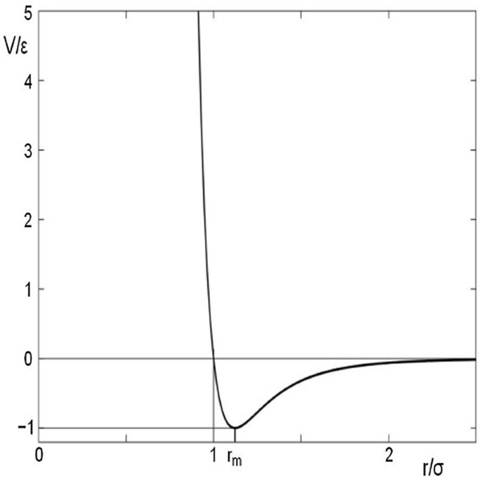

  

  Lennard-Jones interatomic potential

  $$ V(r)=4\varepsilon \left[{\left(\frac{\sigma }{r}\right)}^{12}-{\left(\frac{\sigma }{r}\right)}^6\right] $$

  The term proportional to r⁻¹² represents an empirical fit to the hard-core repulsion produced by the Pauli exclusion at short ranges when the atoms are close enough that the electron orbital overlaps. The r⁻⁶ term represents the van der Waals attraction due to the mutual interactions of the fluctuating dipole moments. Determine the equilibrium separation of two atoms, r_m, in terms of σ and ε.

• 7. Work. Determine the work done by the specified force over the specified paths where ${\hat{e}}_x$ is the unit vector in the x-direction and ${\hat{e}}_y$ is the unit vector in the y-direction. The units of F are newtons and x and y are in meters.

  $$ \overrightarrow{F}=x{\hat{e}}_x+3j{\hat{e}}_y\kern1em \mathrm{and}\kern1em W={\int}_S\overrightarrow{F}\bullet d\overrightarrow{s} $$

• (a) Evaluate the work done by the force along Path S₁, (0, 0) to (2, 0) to (2, 1), with all motion along straight lines.

• (b) Evaluate the work done by the force along Path S₂, which is one straight line directly from (0, 0) to (2,1).

• (c) Evaluate the work along the straight-line Path S₃: (0, 0) to (2, 0) to (2, 1) to (0, 0).

• 8. Similitude. Use dimensional analysis to determine the functional dependence of the variables that describe the following physical systems:

  • (a) Boleadoras. A mass, m, at the end of a string of length, ℓ, is swung overhead. Its tangential velocity is v. Determine the tension in the string. (You may neglect gravity.)

  • (b) Droplet oscillations. A liquid drop of radius, a, and mass density, ρ [kg/m³], may oscillate with its shape being restored to a sphere if the liquid has a surface tension, σ[N/m]. Determine how the period of oscillation could depend upon these three parameters.

  • (c) Deep water ocean waves. Waves on a very deep ocean travel with a speed, v, that depends upon their wavelength, λ, but not upon their amplitude. How should this speed depend upon the wavelength, λ; the acceleration due to gravity, g [m/s²]; and the density of water, ρ [kg/m³]?

  • (d) Shallow-water gravity waves. If the wavelength of a disturbance on the surface of water is much greater than the depth of the water, h_o ≪ λ, the speed of the surface wave depends only upon depth and the acceleration due to gravity. How does the shallow-water gravity wave speed depend upon h_o and g?

  • (e) Capillary waves. At very short wavelengths, λ, the speed of surface waves on water depends upon wavelength; the fluid mass density, ρ; and the surface tension, σ [N/m].

  • (f) Piano string. How should the frequency of a string depend upon its tension, T [N]; its length, ℓ; and its linear mass density, ρ_L [kg/m]?

• 9. Oscillator output impedance. One way to determine the output impedance of an electronic oscillator or an amplifier is to measure the output voltage as a function of load resistance. The oscillator’s internal resistance, R_int, and the load resistance, R_load, form a voltage divider circuit that relates V_out to V_osc, as shown in Fig. 1.20.

Fig. 1.20

An oscillator which produces a constant output voltage, V_osc, will produce voltage, V_out, across a load resistor, R_load, that depends upon the load resistance and the oscillator’s own internal output resistance, R_int

$$ {V}_{\mathrm{out}}={V}_{\mathrm{osc}}\left(\frac{R_{\mathrm{load}}}{R_{\mathrm{int}}+{R}_{\mathrm{load}}}\right)\kern1em \Rightarrow \kern1em \frac{1}{V_{\mathrm{out}}}=\frac{R_{\mathrm{int}}}{V_{\mathrm{osc}}}\frac{1}{R_{\mathrm{load}}}+\frac{1}{V_{\mathrm{osc}}} $$

Table 1.5 provides values of the load resistance, R_load, and the measured output voltage, V_out, corresponding to that load. Linearize the equation, and make a least-squares plot to determine the oscillator’s internal resistance, R_int, and the oscillator’s internal voltage, V_osc.

Table 1.5 Measured values of output voltage, V_out, vs. load resistance, R_load

• 10. Pendulum data analysis. An experiment proceeds as follows: The pendulum is clamped at the 50th mark, approximately 1 m from the attachment point between wire and the pendulous mass. The oscillation period of the pendulum is recorded. The attachment point is raised by 2.00 ± 0.01 cm to the 49th mark (so the wire is shortened by 2.00 cm), and the period of oscillation is measured again. This same procedure is repeated nine more times, producing an 11-element data set containing the approximate wire length, ℓ_i, and oscillation period, T_i, for i = 1, 2, 3, …, 11.

  • (a) Write an algebraic expression for the acceleration due to gravity, g, in terms of the period, T_i; the wire length, l_i; and an undetermined constant, a, that accounts for the unknown distance between the last mark on the wire and the center of gravity of the mass.

  • (b) Rearrange the equation you wrote in part (a) so that the data set can be plotted as a straight line and the slope and intercept of the line can be used to determine the local acceleration due to gravity, g, and the undetermined offset distance, a. Write expressions for g and for a in terms of the slope and the intercept of the straight line.

• 11. Energy released by the first atomic bomb. The first atomic bomb was detonated in Alamogordo, New Mexico, on 16 July 1945. The explosion was captured in a series of photographs like the one shown in Fig. 1.21. Using these photos, G. I. Taylor [32] was able to use similitude to estimate the energy released by the blast based on the rate at which the fire ball expanded, assuming that the fire ball was hemispherical and that the physical size of the source of the energy was very small.

  • (a) Use dimensional analysis to determine the radius of the hemisphere if that radius depends upon time, t; the energy released by the explosion, E; and the density, ρ, of the air. You may assume that the proportionality constant is unity.

  • (b) The blast radius (in meters) as a function of time (in milliseconds) is given in Table 1.6. Plot the radius vs. time using log-log axes, and determine the power law of the best-fit to those data. How close was the exponent that relates time to radius to the value predicted in part (a)?

  • (c) Express your result in part (a) in terms of the energy release, E.

  • (d) Plot R⁵ vs. t² and set the intercept to zero.

  • (e) Using the slope determined in part (d), estimate the energy released by the explosion assuming the density of air is 1.2 kg/m³. Report your result in joules and in kilotons of TNT. (1 kiloton of TNT = 4.184 × 10⁹ J.)

Fig. 1.21

Photo of the first atomic bomb explosion 25 milliseconds after detonation. The diameter of the blast hemisphere is approximately 260 m

Table 1.6 Blast radius

• 12. Fourier synthesis of a sawtooth waveform. The sawtooth waveform occurs when nonlinear effects distort a sinusoidal sound wave into a fully developed shock wave (Fig. 1.22).

Fig. 1.22

Sawtooth waveform

One cycle of a sawtooth wave, with period T and amplitude A, be expressed algebraically.

$$ y(t)=\frac{2 At}{T}-A $$

(1.121)

Write an expression for the sawtooth as a superposition of Fourier components with frequencies f_n = n/T, where n = 1,2,3,…

References

P.M. Morse, K.U. Ingard, Theoretical Acoustics (McGraw-Hill, New York, 1968); ISBN 07-043330-5
U.S. Department of Labor, Occupational Safety & Health Administration (OSHA), Standard No. 1910.95(b)(2): https://www.osha.gov/pls/oshaweb/owadisp.show_document?p_table=standards&p_id=9735
U.S. Standard Atmosphere (National Oceanic and Atmospheric Administration, National Aeronautics and Space Administration, and United States Air Force, Washington, DC); NOAA-S/T 76-1562. U.S. Gov’t. Printing Office, Stock No. 003-17-00323-0 (1976)
R. Courant, Differential & Integral Calculus, 2nd edn. (Blackie & Son, Glasgow, 1937), Ch. 2, §3.9
J. J. Stoker, Nonlinear Vibrations in Mechanical and Electrical Systems (Interscience, New York, 1950); ISBN 978-04-71570-332
A. B. Pippard, The Physics of Vibration (Cambridge University Press, Cambridge, 1989). See Ch. 9; ISBN 0 521 37200 3
L.D. Landau, E.M. Lifshitz, Theory of Elasticity, 2nd edn. (Pergamon, Oxford, 1970). See §7; ISBN 0 08 006465 5
B. Kinsman, Wind Waves (Prentice-Hall, Englewood Cliffs, 1965)
I.S. Gradshteyn, I.M. Ryzhik, Tables of Integrals, Series, and Products, 4th edn. (Academic, New York, 1980); ISBN 0-12-294760-6
M.L. Boas, Mathematical Methods in the Physical Sciences, 2nd edn. (Wiley, New York, 1983). See Ch. 7; ISBN 0-471-04409-1
D. Wells, Are these the most beautiful? Math. Intell. 12(3), 37–41 (1990)
H. Lamb, Dynamical Theory of Sound, 2nd edn. (Edward Arnold & Co., London, 1931) or (Dover, 1960), pg. 54
E.F. Adiutori, Fourier. Mech. Eng. 127(8), 30–31 (2005)
J.W. Strutt (Lord Rayleigh), The principle of similitude. Nature 95, 66–68 (1915)
E. Buckingham, On physically similar systems; illustrations of the use of dimensional equations. Phys. Rev. 4(4), 345–376 (1914)
J.R. Olson, G.W. Swift, Similitude in thermoacoustics. J. Acoust. Soc. Am. 95(3), 1405–1412 (1994)
M. Strasberg, Dimensional analysis of windscreen noise. J. Acoust. Soc. Am. 83(2), 544–548 (1988)
N.R. Hosier, P.R. Donovan, “Microphone Windscreen Performance,” National Bureau of Standards Report NBSIR 79-1559 (Jan. 1979)
Private communication from Thomas J. Hofler
S. Rabinovich, Measurement Errors: Theory and Practice (American Institute of Physics, New York, 1995); ISBN 1-56396-323-X
H.D. Young, Statistical Treatment of Experimental Data (McGraw-Hill, New York, 1962); ISBN 07-072646-9.
R.A. Nelson, M.G. Olsson, The pendulum – Rich physics from a simple system. Am. J. Phys. 54(2), 112–121 (1986). A better, though less readily accessible treatment, is that of G. G. Stokes, Mathematical and Physical Papers (Macmillan, 1905)
F.J. Anscombe, Graphs in statistical analysis. Am. Stat. 27(1), 17–21 (1973)
Ernest Rutherford, F.R.S., 1st Baron Rutherford of Nelson (1871–1937)
P.R. Bevington, Data Reduction and Error Analysis for the Physical Sciences (McGraw-Hill, New York, 1969)
R.A. Fisher, F. Yates, Statistical tables for biological, agricultural and medical research, 6th edn. (Oliver and Boyd, London, 1963)
L.M. Ronsse, L.M. Wang, Relationships between unoccupied classroom acoustical conditions and elementary student achievement in eastern Nebraska. J. Acoust. Soc. Am. 133(3), 1480–1495 (2013)
J. Higbie, Uncertainty in the linear regression slope. Am. J. Physiol. 59(2), 184–185 (1991)
Y. Beers, Introduction to the Theory of Error, 2nd edn. (Addison-Wesley, Reading, 1957)
J. W. Strutt (Lord Rayleigh), The Theory of Sound, vol I, 2nd edn. (Macmillan, London, 1894) reprinted (Dover, 1945)
J.E. Lennard-Jones, On the determination of molecular fields. Proc. R. Soc. Lond. A 106, 463–477 (1924)
G.I. Taylor, The formation of a blast wave by a very intense explosion. II. The atomic explosion of 1945. Proc. Roy. Soc. Lond 201(1065), 175–186 (1950)
Author information
Authors and Affiliations
Rights and permissions
Open Access This chapter is licensed under the terms of the Creative Commons Attribution 4.0 International License (http://creativecommons.org/licenses/by/4.0/), which permits use, sharing, adaptation, distribution and reproduction in any medium or format, as long as you give appropriate credit to the original author(s) and the source, provide a link to the Creative Commons license and indicate if changes were made.
The images or other third party material in this chapter are included in the chapter's Creative Commons license, unless indicated otherwise in a credit line to the material. If material is not included in the chapter's Creative Commons license and your intended use is not permitted by statutory regulation or exceeds the permitted use, you will need to obtain permission directly from the copyright holder.
Copyright information
© 2020 The Author(s)
About this chapter
Cite this chapter
Garrett, S.L. (2020). Comfort for the Computationally Crippled. In: Understanding Acoustics. Graduate Texts in Physics. Springer, Cham. https://doi.org/10.1007/978-3-030-44787-8_1
Download citation
DOI: https://doi.org/10.1007/978-3-030-44787-8_1
Published:
Publisher Name: Springer, Cham
Print ISBN: 978-3-030-44786-1
Online ISBN: 978-3-030-44787-8
eBook Packages: Physics and AstronomyPhysics and Astronomy (R0)