Corporate Income Tax: WACC, FTE, TCF, APV

Abstract

There is a variety of problems in the valuation of firms. That is why the evaluator has to make some simplifications in order to come up with a result. That also goes for the theory of valuation. We will take the first step in assuming that the firm has no debt. In simplifying with this assumption, we shall see that a number of economic problems can be discussed. In the next step we will turn to indebted firms.

There is a variety of problems in the valuation of firms. That is why the evaluator has to make some simplifications in order to come up with a result. That also goes for the theory of valuation. We will take the first step in assuming that the firm has no debt. In simplifying with this assumption, we shall see that a number of economic problems can be discussed. In the next step we will turn to indebted firms.

3.1 Unlevered Firms

Whoever has to value levered firms, also has to be able to value unlevered firms. Both are mutually conditional.

By itself, this claim does not shed any light. It should be understood that if a levered firm is spoken of without naming any further details, then that remains unclear. Are we dealing with a heavily or only moderately levered firm? Will the firm’s debt increase, or are the responsible managers planning to reduce the firm’s credit volume? In contrast to a levered firm in which this must all be explained in detail, the circumstances of an unlevered firm are clear and simple. When we speak of an unlevered firm, we mean a firm, which will not have debts today, nor anytime in the future. Of course it is difficult to believe that there are actually such firms in our world. But this—no doubt fully correct assessment—does not matter here. All we want to state is that what we mean by an unlevered firm is completely straightforward, while by a levered firm it is not so clear without further information.

Cost of Capital and Leverage

A firm’s cost of capital essentially depends upon two influences: firstly, the firm’s business risk, and secondly, its indebtedness. It is fundamentally valid that the greater the risk is and the greater the firm’s debt-equity ratio is, that much higher the expected returns are. And if we make the connection between this law and the considerations of the preceding paragraph, then the cost of capital of an equity-financed firm is straightforward, while the cost of capital of an indebted firm is dependent upon the level of debt. Of course this is all only valid so long as we keep all other influences upon the cost of capital—particularly the business risk and the tax rate—constant.

The indebted firm’s cost of capital is needed in order to be able to correctly value it. To put it more exactly: the cost of capital is needed of a firm, which has two things in common with the firm to be valued. These regard, namely, its business risk and its debt. If you want to determine this cost of capital by using empirical data from the capital market, you typically get into the following situation. You go to the trouble of finding a firm that belongs to the same, or at least very similar risk class (comparison firm) and estimate the expected value of the returns, which the financiers receive. In doing so you almost always have to observe that the comparison firm is financed differently than the firm to be valued. But if the debt now has an influence on the amount of the cost of capital, the comparison firm’s cost of capital cannot simply be applied to the firm to be valued. As we already made clear, indebted firms are not necessarily comparable even when they belong to the same risk class. And it is exactly here that the equity-financed firm comes into play as reference firm.

The indebted firm, this will become clear in a moment, is under any circumstances more valuable than an equity-financed company with identical cash flows. Hence, raising debt will serve as a leverage that can increase the firm’s value. In this case one also speaks of a leverage effect caused by debt. That is why we will use the expressions indebted and levered as well as equity-financed and unlevered as synonyms.

Unlevering and Relevering

In order to determine the cost of capital of the firm to be valued, the comparison firm’s cost of capital is to be adjusted because of the reasons described here. Academics, who are involved with the theoretical side of valuation of firms, have to develop functional equations, which allow for the cost of capital of the—levered—comparison firm to be converted into the unlevered firm’s cost of capital. If they are successful, then the equations can be used to infer the reference firm’s cost of capital from the comparison firm’s cost of capital (unlevering), but also to infer the cost of capital of the firm to be valued from the reference firm’s cost of capital (relevering).

And thus the circle is complete: whoever wants to value a levered firm, must also be able to value an unlevered firm. The academics are then naturally required to live up to the expectations placed on them and must actually be in the position to develop the necessary adjustment equations. Should they fail at this, then the discounting of levered firms’ cash flows with the appropriate cost of capital must simply be forgotten.

Notation

In the first chapter of this book, we spoke of free cash flows and firm values without troubling ourselves with how the firms are financed. Now we are concentrating on firms, which are completely equity-financed. Therefore, the relevant symbols get an appropriate index. We use a superior u for unlevered firms. We will, for instance, designate the free cash flows after corporate income taxes of such firms with $\widetilde {\mathit {FCF}}^u_t$, and the firm values with $\widetilde {V}^u_t$. Notice that since only cash flows after taxes can be paid to the owners of the firm, $\widetilde {\mathit {FCF}}^u_t$ will denote free cash flows after corporate income tax. Unlevered firms have only one single group of financiers. For the returns that the owners are expecting we will use the symbol $\widetilde {k}^{E,u}_t$.

3.1.1 Valuation Equation

We assume in the following that it is possible to successfully come up with the required adjustment equations and will actively attempt to do so ourselves as best we can. Under this condition, the cost of capital of the totally equity-financed firm can be considered to be known. We assume that the evaluator knows the unlevered firm’s conditional expected free cash flows $\operatorname *{\mathrm {E}}\left [\widetilde {\mathit {FCF}}^u_s|\mathcal {F}_t\right ]$ for time s = t + 1, …, T.

Definition 3.1 (Cost of Capital of the Unlevered Firm)

Cost of capital $\,\widetilde {k}^{E,u}_t$ of an unlevered firm are conditional expected returns

$$\displaystyle \begin{aligned} \widetilde{k}^{E,u}_t:=\frac{\operatorname*{\mathrm{E}}\left[\widetilde{\mathit{FCF}}^u_{t+1}+\widetilde{V}^u_{t+1}|\mathcal{F}_t\right]}{\widetilde{V}^u_t}-1.\end{aligned} $$

The reader should notice that we use the cash flows after corporate income tax in our definition of cost of capital. Therefore, $k^{E,u}_t$ are variables after corporate income tax, too. The question, how we can defer from these any cost of capital before tax is not our concern, since we do not investigate how the value of a company changes with a changing of the tax rate. Although possibly time dependent, our tax rates are fixed once and for all today. Nevertheless, if anyone tries to determine the cost of capital before tax he cannot operate on grounds of our theory since it does not tell anything about how the value of a firm changes with the tax rates.

The valuation of the unlevered firm is absolutely unproblematic under these conditions.

Theorem 3.1 (Market Value of the Unlevered Firm)

If the cost of capital of the unlevered firm $k^{E,u}_t$ are deterministic, then the value of the firm, which is only financed with owners’ equity, amounts at time t to

$$\displaystyle \begin{aligned} \widetilde{V}^u_t=\sum_{s=t+1}^T\frac{\operatorname*{\mathrm{E}}\left[\widetilde{\mathit{FCF}}^u_{s}|\mathcal{F}_t\right]}{\left(1+k^{E,u}_{t}\right)\ldots \left(1+k^{E,u}_{s-1}\right)}\;. \end{aligned}$$

We do not have to further involve ourselves here with the proof of the assertion. We already handled it in a generalized form in Sect. 2.3.3 and do not need to bore our readers here by repeating ourselves.¹

3.1.2 Weak Auto-Regressive Cash Flows

In Theorem 3.1 we determined a valuation equation for unlevered firms that the evaluator can only use if she knows the cost of equity of the unlevered firm. This condition can only very rarely be counted upon in practice. If the required conditions to use the theorem are not met, then the valuation is anything but a trivial problem.

Cash Flows of the Unlevered Firm

You can only get further in such a situation if the adjustment equation already mentioned above is available. The derivation of such an equation is, however, only possible if the appropriate suppositions are met. In the following sections of this book we will develop adjustment equations for demanding cases. Our results are indeed based on a special condition regarding the structure of the unlevered firm’s free cash flows after taxes. From now on we will assume that the cash flows form a so-called weak auto-regressive process.² The reader may rest assured that without recourse to this assumption, development of correct adjustment formulas is doomed to fail.

Assumption 3.1 (Weak Auto-Regressive Cash Flows)

There are real numbers g_t > −1 such that

$$\displaystyle \begin{aligned} \operatorname*{\mathrm{E}}\left[\widetilde{\mathit{FCF}}^u_{t+1}|\mathcal{F}_t\right]=(1+g_{t})\,\widetilde{\mathit{FCF}}^u_t \end{aligned}$$

is valid for the unlevered firm’s cash flows after taxes.

We must assume that g_t is greater than − 100% in order to prevent cash flows from having oscillating signs which would be rather unrealistic. It is not necessary to assume that g_t is positive, so shrinking cash flows are not excluded with Assumption 3.1.

Uncorrelated (Additive) Increments

In order to understand this assumption, we firstly look at the increments of the cash flow process. In formal notation we thus have

$$\displaystyle \begin{aligned} \widetilde{\mathit{FCF}}^u_{t+1}=(1+g_{t})\,\widetilde{\mathit{FCF}}^u_t+ \varepsilon_{t+1}. \end{aligned} $$

(3.1)

g_t is a deterministic amount that is already known in t = 0. What does our assumption on weak auto-regressive cash flows imply for the increments ε_t+1? It will imply that these increments have expectation zero and are uncorrelated to each other (sometimes called “white noise” although this in fact refers to independent increments).

It is not immediately recognizable that this assumption really implies uncorrelated noise terms. In order to prove that, we have to carry out a little calculation. In doing so, we will again make use of the rules for conditional expectations. We first of all show that the noise terms’ expectation disappears,³

$$\displaystyle \begin{aligned} \operatorname*{\mathrm{E}} \left[ \varepsilon_{t+1}\right] &= \operatorname*{\mathrm{E}} \left[ \varepsilon_{t+1} |\mathcal{F}_0\right] && \text{Rule 1}\\ &= \operatorname*{\mathrm{E}} \left[ \operatorname*{\mathrm{E}}\left[ \varepsilon_{t+1}|\mathcal{F}_t\right] |\mathcal{F}_0 \right] && \text{Rule 4}\\ &=\operatorname*{\mathrm{E}} \left[ \operatorname*{\mathrm{E}}\left[\widetilde{\mathit{FCF}}^u_{t+1}-(1+g_{t})\widetilde{\mathit{FCF}}^u_t|\mathcal{F}_t\right] |\mathcal{F}_0 \right] && \text{by (3.1)}\\ &=\operatorname*{\mathrm{E}} \left[ \operatorname*{\mathrm{E}}\left[\widetilde{\mathit{FCF}}^u_{t+1}|\mathcal{F}_t\right] -(1+g_{t})\operatorname*{\mathrm{E}}\left[\widetilde{\mathit{FCF}}^u_t|\mathcal{F}_t\right] |\mathcal{F}_0 \right] && \text{Rule 2}\\ &=\operatorname*{\mathrm{E}} \left[ \operatorname*{\mathrm{E}}\left[\widetilde{\mathit{FCF}}^u_{t+1} |\mathcal{F}_t \right] -(1+g_{t})\widetilde{\mathit{FCF}}^u_t |\mathcal{F}_0 \right] && \text{Rule 5}\\ &= \operatorname*{\mathrm{E}} \left[0 |\mathcal{F}_0\right] && \text{Assumption 3.1}\\ &=0 \,. \end{aligned} $$

Now we come to the proof that the noise terms are uncorrelated. We look at two points in time s < t and have to show that the covariance Cov[ε_s, ε_t] disappears. We already know that the noise terms’ expectations are zero. And so from the covariance it immediately follows:

$$\displaystyle \begin{aligned} \text{Cov} [ \varepsilon_s, \varepsilon_t] & = \operatorname*{\mathrm{E}} \left[ \varepsilon_s \varepsilon_t\right] - \operatorname*{\mathrm{E}} \left[ \varepsilon_s\right] \operatorname*{\mathrm{E}} \left[ \varepsilon_t\right] \\ & = \operatorname*{\mathrm{E}} \left[ \varepsilon_s \varepsilon_t\right] \,. \end{aligned} $$

From the rules as well as from the definition of noise term it follows:

$$\displaystyle \begin{aligned} \text{Cov}[ \varepsilon_s, \varepsilon_t]&=\operatorname*{\mathrm{E}}\left[ \varepsilon_s \varepsilon_t\right]\\ &= \operatorname*{\mathrm{E}}\left[ \varepsilon_s \varepsilon_t|\mathcal{F}_0\right]&&\text{Rule 1}\\ &= \operatorname*{\mathrm{E}}\left[\operatorname*{\mathrm{E}}\left[ \varepsilon_s \varepsilon_t|\mathcal{F}_s\right]|\mathcal{F}_0\right]&&\text{Rule 4}\\ &= \operatorname*{\mathrm{E}}\left[ \varepsilon_s\operatorname*{\mathrm{E}}\left[ \varepsilon_t|\mathcal{F}_s\right]|\mathcal{F}_0\right].&&\text{Rule 5} \end{aligned} $$

Now we concentrate on the conditional expectation, which comes up in the last equation and get the following from the rules as well as the fact that cash flows are weak auto-regressive:

$$\displaystyle \begin{aligned} \operatorname*{\mathrm{E}}\left[ \varepsilon_{t}|\mathcal{F}_s\right] &= \operatorname*{\mathrm{E}}\left[\widetilde{\mathit{FCF}}^u_{t}-(1+g_{t-1})\widetilde{\mathit{FCF}}^u_{t-1}|\mathcal{F}_s\right] \\ &= \operatorname*{\mathrm{E}}\left[\operatorname*{\mathrm{E}}\left[\widetilde{\mathit{FCF}}^u_{t}-(1+g_{t-1})\widetilde{\mathit{FCF}}^u_{t-1}|\mathcal{F}_{t-1}\right]|\mathcal{F}_s\right] &&\text{Rule 4}\\ &= \operatorname*{\mathrm{E}}\left[\operatorname*{\mathrm{E}}\left[\widetilde{\mathit{FCF}}^u_{t}|\mathcal{F}_{t-1}\right]-(1+g_{t-1})\widetilde{\mathit{FCF}}^u_{t-1}|\mathcal{F}_s\right] &&\text{Rule 2, 5}\\ &=0\,. &&\text{Assumption 3.1} \end{aligned} $$

The covariance disappears, which is exactly what we wanted to show.

Independent (Additive) Increments

Until now, we have proven that the vanishing expectation of the noise terms ε_t+1 as well as their uncorrelation results from the Assumption 3.1. You may get the impression that the reverse is true as well. This is not the case. For reasons of order, we have to ascertain that it is the condition

$$\displaystyle \begin{aligned} \operatorname*{\mathrm{E}}\left[\varepsilon_{t+1}|\mathcal{F}_t\right]=\operatorname*{\mathrm{E}}\left[\varepsilon_{t+1}\right] (=0)\,, \end{aligned}$$

which is logically sufficient to weak auto-regressive cash flows.

To understand this condition, we refer to the fact that numerous financial models work on the assumption that a firm’s free cash flows would follow a random walk. What does that mean? It means that the cash flows possess increments, which are independent from each other and distributed identically. The noise terms ε_t+1 have an expectation of zero, are distributed identically and are mutually independent.

This is a big assumption, far bigger than the one we made. The independence of the noise terms implies, for instance, that the increments of the cash flow in t is not connected to the cash flows from years 1 to t − 1. If we have been looking at continuously growing cash flows in the last few years, that by no means suggests that this growth will remain in year t. You cannot draw any conclusions in the least from the development of the years 1 to t − 1 for the year t! Uncorrelation in contrast does not pose such a strong challenge.

While uncorrelation excludes only a linear relation, independence negates every single causal relation: In our notation independence is equivalent to

$$\displaystyle \begin{aligned} \operatorname*{\mathrm{E}}\left[f(\varepsilon_{t+1})|\mathcal{F}_t\right]=\operatorname*{\mathrm{E}}\left[f(\varepsilon_{t+1})\right] \end{aligned}$$

for any function f(x).⁴ Compare this to the equation above, where f needs only to be linear. If the equation does not hold for any linear function, then there may well be any other nonlinear functional relation f. Independent random variables have always correlation zero, but uncorrelated random variables are—apart from normally distributed random variables—not independent from each other. This again makes clear that in the assumption on weak auto-regressive cash flows we are dealing with a weaker formulation. We are not insinuating any random walk with regard to the cash flows within the framework of our theory, but are instead working on the basis of the less demanding uncorrelated growth.

Multiplicative Versus Additive Increments

Understanding auto-regressive cash flows is not an easy task. In the previous section, we looked at additive increments of cash flows in order to find an appropriate way of interpretation. But the additive context is by no means compelling. We could have used a multiplicative link as well. In the following, we will briefly discuss this and show that the result does not change at all. So, whether we go the additive or a multiplicative path is pure taste. A multiplicative relation is defined by

$$\displaystyle \begin{aligned} \widetilde{\mathit{FCF}}^u_{t+1}=(1+g_{t})\,\widetilde{\mathit{FCF}}^u_t \left(1+ \varepsilon_{t+1}\right). \end{aligned} $$

(3.2)

First, we will check which properties of the error terms ε_t guarantee that the cash flows turn out to be weak auto-regressive once again. By inserting Assumption 3.1 in the definition we get

$$\displaystyle \begin{aligned} (1+g_t)\widetilde{\mathit{FCF}}^u_t&=\operatorname*{\mathrm{E}}[\widetilde{\mathit{FCF}}^u_{t+1}|\mathcal{F}_t]&\text{Assumption 3.1}\\ &=(1+g_{t})\cdot\widetilde{\mathit{FCF}}^u_t \cdot\left(1+ \operatorname*{\mathrm{E}}[\varepsilon_{t+1}| \mathcal{F}_t]\right)&\text{Rule 5}. \end{aligned} $$

This means that

$$\displaystyle \begin{aligned} \operatorname*{\mathrm{E}}[\varepsilon_{t+1}|\mathcal{F}_t]=0 \end{aligned}$$

is sufficient and necessary for weak auto-regression. Differences between additive and multiplicative increments only play a role when the distributions of the error terms come into play. However, these differences are not important in the following. The result can also be seen by taking the logarithm on both sides of Eq. (3.2),

$$\displaystyle \begin{aligned} \log\left(\widetilde{\mathit{FCF}}^u_{t+1}\right)=\log \left((1+g_t)\widetilde{\mathit{FCF}}^u_t \right) +\log\left(1+ \varepsilon_{t+1}\right). \end{aligned}$$

In a multiplicative model the logarithms of the cash flows follow an additive model with $\log \left (1+\varepsilon _{t+1}\right )$ representing the error terms.⁵ Based on these considerations we will restrict ourselves on additive error terms from now on.

Justification of Weak Auto-Regressive Cash Flows

Every economic theory is based on assumptions. The numerous jokes usually told about us economists are based on the fact that we occasionally apply unrealistic, odd conditions. Economists who would like to be taken seriously must put up with the question as to whether their assumptions are justifiable. May we actually insinuate in good conscience that the Assumption 3.1 is met in terms of a firm’s free cash flows? Isn’t this assumption perhaps totally “far-fetched”?

From our experience, practically engaged evaluators normally do not deal at all with the question as to which distribution laws uncertain future cash flows follow. On the contrary they limit themselves to estimating the expectations of these future cash flows. It can now be shown that there are always state spaces with upwards and downwards movements like that analogous to Fig. 2.2 for whatever sequence of expectations you like. Assumption 3.1 is thus met in this model.⁶ But that does not mean anything else than that an evaluator working with estimated expectations of cash flows can operate upon the basis that—so to speak behind the scenes—there is always a state space that corresponds to the Assumption 3.1. All in all, that is why we hold the assumption on weak auto-regressive cash flows to be practically acceptable.

The question can be raised at this point as to why exactly the unlevered firm’s cash flows should be weak auto-regressive. It is obvious that our Assumption 3.1 is arbitrary and it does not make any sense to hide that. Couldn’t we have just as well replaced our assumption with the condition that the free cash flows of a levered firm are weak auto-regressive? Could this levered firm be chosen in just any way, or would it have to be a firm with a particular financing policy? We must give a clear answer to the questions raised here: Varying results would be gotten in any case for the valuation equations, which we will be developing in the following. What is more, we think the following ascertainment is important: If it were to be supposed that a levered firm has weak auto-regressive cash flows, then it would not necessarily follow that the free cash flows of a firm with a different financing policy have this same characteristic as well.⁷

Conclusions from Weak Auto-Regressive Cash Flows: Dividend-Price Ratio

If cash flows are weak auto-regressive, then it can be proven that the unlevered firm’s value is a multiple of the free cash flow. To put it differently, the unlevered firm must always show a deterministic dividend-price ratio. This result is well-known in the case of a perpetual rent from the Williams/Gordon-Shapiro formula.

Theorem 3.2 (Williams/Gordon-Shapiro Formula)

If the cost of capital is deterministic and cash flows are weak auto-regressive, then for the value of the unlevered firm

$$\displaystyle \begin{aligned} \widetilde{V}^u_t=\frac{\widetilde{\mathit{FCF}}^u_t}{d^u_t} \end{aligned}$$

holds for deterministic and positive $d^u_t>0$ which will be called dividend-price ratio.

We have banned the proof for this theorem to the appendix.

The last proposition shows that the expected capital gains of the unlevered firm rate is deterministic

$$\displaystyle \begin{aligned} \frac{\operatorname*{\mathrm{E}}\left[\widetilde{V}^u_{t+1}|\mathcal{F}_t\right]-\widetilde{V}^u_t}{\widetilde{V}^u_t}= \frac{\left(d^u_{t+1}\right)^{-1}\operatorname*{\mathrm{E}}\left[\widetilde{\mathit{FCF}}^u_{t+1}\right]}{\left(d^u_t\right)^{-1}\widetilde{\mathit{FCF}}^u_t}-1=\frac{d^u_{t}(1+g_{t})}{d^u_{t+1}} -1 \end{aligned}$$

and is zero in particular if the dividend-price ratio is constant and the growth rate is zero.

Conclusions from Weak Auto-Regressive Cash Flows: Discount Rates

We had already made it clear in the introduction that for the case under certainty, the returns and not the yields present the appropriate means of determining the value of cash flows. Now we take up the question as to the relation which exists between returns and discount rates. Let us take a look in order to get a certain idea of the free cash flows of any year you like. Without further assumptions on the capital market, we cannot act as if a claim to this single cash flow will be traded. Otherwise, the owner of a share would have claims to dividends, so to speak, but not to the share price of the security. Nevertheless, the question that we want to ask ourselves is: what price should an investor pay at time t < s for an isolated free cash flow $\widetilde {\mathit {FCF}}^u_s$?

Although we have not precisely developed the basic elements of the arbitrage theory, we may make use of the fundamental theorem in terms of an analogous argument. If we can actually value levered as well as unlevered firms with this principle, then this should also be possible for the claim to an isolated cash flow. This cash flow is valued by constituting the expectation in terms of the risk-neutral probability and then discounting it with the riskless rate,⁸

$$\displaystyle \begin{aligned} \frac{\operatorname*{\mathrm{E}}\nolimits_Q\left[\widetilde{\mathit{FCF}}^u_{s}|\mathcal{F}_t\right]}{(1+r_f)^{s-t}}\;. \end{aligned}$$

The above expression gives the value of the free cash flows $\widetilde {\mathit {FCF}}^u_s$ at time t. It is immediately noticeable that this valuation formula, albeit extremely elegant, is totally useless: we know next to nothing about the probability measure Q. We will now turn our attention to a second outcome, which can be gotten from the fact that cash flows are weak auto-regressive. If cash flows are weak auto-regressive, then there is another way to value them which is of interest to us. In order to let that become clear, we must precisely define the term discount rate, which has until now been only vaguely introduced. For that we will make use of a few preliminary considerations.

Under the discount rate κ_t we understand that number, which allows the price of the cash flow $\widetilde {\mathit {FCF}}^u_{t+1}$ at time t to be determined. According to our statements up to present, the discount rate κ_t shall serve as an instrument to value the single cash flow $\widetilde {\mathit {FCF}}^u_{t+1}$, or using the subjective probabilities we must have

$$\displaystyle \begin{aligned} \frac{\operatorname*{\mathrm{E}}\left[\widetilde{\mathit{FCF}}^u_{t+1}|\mathcal{F}_t\right]}{1+\kappa_t}=\frac{\operatorname*{\mathrm{E}}_Q\left[\widetilde{\mathit{FCF}}^u_{t+1}| \mathcal{F}_t\right]}{1+r_f}\;. \end{aligned} $$

(3.3)

Yet, this consideration alone is not sufficient for our purposes. We do not simply want to make use of the discount rates to value cash flows, which are each one single period away from the time of valuation. If we are, for instance, dealing with the valuation of the cash flow $\widetilde {\mathit {FCF}}^u_{t+2}$ at time t, then we want to manage this task with two discount rates, namely with κ_t as well as with κ_t+1 in just such a way that

$$\displaystyle \begin{aligned} \frac{\operatorname*{\mathrm{E}}\left[\widetilde{\mathit{FCF}}^u_{t+2}| \mathcal{F}_t\right]}{(1+\kappa_t)(1+\kappa_{t+1})}=\frac{\operatorname*{\mathrm{E}}_Q\left[\widetilde{\mathit{FCF}}^u_{t+2}|\mathcal{F}_t\right]}{\left(1+r_f\right)^2} \end{aligned} $$

(3.4)

is valid. But now it is not so unmistakably clear whether κ_t is serving the valuation of the cash flow $\widetilde {\mathit {FCF}}^u_{t+1}$ or the cash flow $\widetilde {\mathit {FCF}}^u_{t+2}$. And we can also no longer assume that the discount rate κ_t from Eq. (3.3) agrees with κ_t from Eq. (3.4).⁹ We will thus suggest a definition for the discount rates that takes the cash flows to be valued into consideration and which requires a somewhat more complicated notation.

Definition 3.2 (Discount Rates of the Unlevered Firm)

Real numbers $\kappa ^{t\to s}_t, \kappa ^{t\to s}_{t+1} \ldots$ are called discount rates of the cash flow $\widetilde {\mathit {FCF}}^u_s$ of the unlevered firm at time t, if they satisfy

$$\displaystyle \begin{aligned} \frac{\operatorname*{\mathrm{E}}\nolimits_Q\left[\widetilde{\mathit{FCF}}^u_{s}|\mathcal{F}_t\right]}{(1+r_f)^{s-t}}= \frac{\operatorname*{\mathrm{E}}\left[\widetilde{\mathit{FCF}}^u_{s}|\mathcal{F}_t\right]}{\left( 1+\kappa^{t\to s}_{t}\right)\ldots \left(1+\kappa^{t\to s}_{s-1}\right)}\;.\end{aligned} $$

We stress that this is only one of many conceivable definitions. We could, for instance, also define the discount rates as yields instead of the version we have chosen. If we do not do so, it is due solely to practical considerations.

We can, on the basis of definition (3.2), clarify the question as to whether the cost of capital k^{E, u} prove to be appropriate candidates for discount rates of the unlevered cash flows. In answering this question we fall back upon the assumption that the cash flows of the unlevered firm are weak auto-regressive. Cost of capital does not then just only prove itself as appropriate discount rates. It has, much further, the pleasant characteristic that it is independent of the particular cash flow to be valued $\widetilde {\mathit {FCF}}^u_s$. This characteristic will later prove itself to be very helpful.

Theorem 3.3 (Equivalence of the Valuation Concepts)

If the cost of capital is deterministic and the cash flows of the unlevered firm are weak auto-regressive, then the following is valid for all times: s > t

$$\displaystyle \begin{aligned} \frac{\operatorname*{\mathrm{E}}\nolimits_Q\left[\widetilde{\mathit{FCF}}^u_{s}|\mathcal{F}_t\right]}{\left(1+r_f\right)^{s-t}}= \frac{\operatorname*{\mathrm{E}}\left[\widetilde{\mathit{FCF}}^u_{s}|\mathcal{F}_t\right]}{\left( 1+k^{E,u}_{t}\right)\ldots \left(1+k^{E,u}_{s-1}\right)} \;. \end{aligned}$$

This is the same as to say that cost of capital are indeed discount rates regardless of s > t ≥ τ

$$\displaystyle \begin{aligned} \kappa^{s\to \tau}_t=k^{E,u}_t\;. \end{aligned}$$

That this theorem follows from the met assumptions can hardly be so easily recognized. Since the proof would demand a fair amount of space and perhaps not even be of interest to every reader, we have banned it to an appendix.¹⁰

Critical readers could suspect that this theorem has to do with a simple application of the definition of the cost of capital. This would most definitely be a wrong conclusion and in order to make it more understandable, we would like to go into it in more detail. Just equating Eq. (2.8) with Theorem 3.1 leads us in terms of unlevered firms to the result

$$\displaystyle \begin{aligned} \widetilde{V}^u_t=\sum_{s=t+1}^T\frac{\operatorname*{\mathrm{E}}_Q\left[\widetilde{\mathit{FCF}}^u_{s}|\mathcal{F}_t\right]}{\left(1+r_f\right)^{s-t}} =\sum_{s=t+1}^T\frac{\operatorname*{\mathrm{E}}\left[\widetilde{\mathit{FCF}}^u_{s}|\mathcal{F}_t\right]}{\left(1+k^{E,u}_{t}\right)\ldots \left(1+k^{E,u}_{s-1}\right)}\;. \end{aligned}$$

The preceding equation is of little surprise, as it only claims the equivalence of two different ways of calculation: either the risk-neutral probability and the riskless interest rate is used, or the evaluator applies the subjective probability and the (correspondingly) defined cost of capital. Since the cost of capital is now so defined that both expressions give identical values, there is no reason to worry about coming up with equal firm values.

Of surprise, however, is the declaration that not only do the sums agree in the last equation, but the summands as well. This is everything but obvious, as the simple example

$$\displaystyle \begin{aligned} 4+6=3+7 \qquad \text{but } 4\neq 3 \text{ and } 6\neq 7 \end{aligned}$$

shows. The reader should keep both statements (i.e., the identity of the sums as well as the identity of the summands) clearly separate. Our statement is everything but self-evident and is thoroughly in need of a proof.

A First Look at Default

Until now we had purposely not included the case in which the firm to be valued can go bankrupt. But as the company grows, the probability of going into default is increasing.

If the court in charge allows for the commencement of bankruptcy proceedings, the consequences for creditors, suppliers, employees, owners, and managers are determined in detail by the bankruptcy law. As a rule a liquidator is placed in charge of the business affairs and examines how each party’s payment claims can best be settled. The liquidator makes suitable suggestions within a given time frame and tries to get the agreement of the creditors and the court.

There are principally three possibilities. You can try to rehabilitate the firm, that is, to re-establish the profitability through suitable restructuring measures. In order to do this, the creditors must be willing to renounce some of their claims. If that is not feasible, then the insolvent firm can be transferred over to a bail-out firm and the creditors are paid off by the sales proceeds. If such a solution is also not practical, then there is no other option than to close down and liquidate the firm. What then remains is the smaller the faster the breakup of the firm takes place.

In the following we only assume that in determining future cash flows as well as in laying down future financing and investment policies, all conceivable developments were taken into consideration. If all conceivable developments are being spoken of, then that also includes situations in which the firm goes into default or has gone into default.

Unlevered firms can go bankrupt if claims of tax authorities, employees, and the like are not satisfied. Formal insolvency proceedings are regulated differently from one jurisdiction to the other. However, most countries apply similar default triggers. Usually, illiquidity and over-indebtedness are typical default triggers. A company gets illiquid if its net cash flows (i.e., cash flows to equity or CFE) are negative. A company is over-indebted if the value of equity is negative (whereas market as well as book values are being used in this definition).¹¹ Similarly, e.g., the UK Insolvency Act initiates bankruptcy proceedings if a firm either does not have enough assets to cover its debts (i.e., the value of assets is less than the amount of the liabilities), or it is unable to pay its debts as they fall due.

Let us first concentrate on the case of an unlevered firm. It is tempting to suggest that an unlevered company is illiquid if the owners’ net cash flows turn out to be negative or $\widetilde {\mathit {FCF}}^u_t(\omega )<0$. But it is clearly apparent that this definition has its pitfalls when used in a DCF context. Why do we have to emphasize this? If net cash flows are positive, the company pays money to the owners. But if not, it is just the other way round: the owners pay money to the company if net cash flows appear to be negative. Now, if a sufficient amount of money is paid to the company, the firm is no longer illiquid. The owners simply rectify the unpleasant situation. Hence, if and only if the owners do not completely comply with their reserve liabilities, one can actually speak of a lack of liquidity of the company.

We hold the following: whenever the owners cannot or do not meet their funding obligations, the company effectively faces illiquidity.¹² However, the mere existence of negative net cash flows does not automatically imply such a run of events. We should therefore speak of the danger of illiquidity that arises if net cash flows turn out to be negative or $\widetilde {\mathit {FCF}}^u_t(\omega )<0$.

Let us now turn to over-indebtedness as the second default trigger. How could this term be interpreted when we look at an unlevered firm? We will characterize such a situation by $\widetilde {V}^u_t(\omega )<0$. If this condition is fulfilled, from the owner’s point of view continuing the business would be out of the question. It would undoubtedly be appropriate to speak of “not continuable unlevered firms.” However, for systematic reasons we use the terms “in danger of illiquidity” and “in danger of negative equity,” provided the mentioned inequality is met.

The following proposition will show that now over-indebtedness and danger of illiquidity are in the case of unlevered firms merely equivalent. Both default triggers in fact turn out to coincide and it was too much of an effort to distinguish both cases. But it will turn out that in the case of a levered firm things will become much more complicated.

Theorem 3.4 (Default of the Unlevered Firm)

Consider an unlevered firm with weak auto-regressive cash flows. If the company is in danger of illiquidity at date t in some state, it will also be in danger of negative equity at the same date for the same state.

This immediately follows from Proposition 3.2.

Notice that the market value of equity for corporations cannot be negative, since they have limited liability. The market value of non-corporations, say partnerships, can be negative though. This is the reason why we speak only of danger of insolvency instead of insolvency itself. Our theorem mainly discloses how a consistent valuation model even of an unlevered firm has to be built in order to avoid such logical contradictions.

We now have the basic elements of our theory on discounted cash flow. In the following sections it must be shown what can be done with these basic elements.

3.1.3 Example (Continued)

The Finite Case

Beforehand we want to take up our example from Sect. 2.2.3 and establish the value of the unlevered firm. As we have seen the cash flows follow a weak auto-regressive development. In addition, we assume that the cost of capital of the unlevered firm is constant in time and amounts to 20%. According to Theorem 3.1, it is obvious what market value the unlevered firm has at time t = 0,

$$\displaystyle \begin{aligned} \text{V}^u_0&= \frac{\operatorname*{\mathrm{E}}\left[\widetilde{\mathit{FCF}}^u_1\right]}{1+k^{E,u}}+\frac{\operatorname*{\mathrm{E}}\left[\widetilde{\mathit{FCF}}^u_2\right]}{(1+k^{E,u})^2}+\frac{\operatorname*{\mathrm{E}}\left[\widetilde{\mathit{FCF}}^u_3\right]}{(1+k^{E,u})^3}\\ &=\frac{100}{1.2}+\frac{110}{1.2^2}+\frac{121}{1.2^3}\approx 229.75\;. \end{aligned} $$

Although the use of this calculation is perhaps not recognizable yet here, we want to determine the market value of the unlevered firm for time t = 1 as well. This is not clear, because we cannot yet know today, if the outcome at time t = 1 will result in the condition up or down. Depending upon the condition, we are discounting different cash flows. In the condition of up, we get¹³

$$\displaystyle \begin{aligned} \widetilde{V}^u_1(u) &=\frac{\operatorname*{\mathrm{E}}\left[\widetilde{\mathit{FCF}}^u_2(\omega|u)\right]}{1+k^{E,u}} + \frac{\operatorname*{\mathrm{E}}\left[\widetilde{\mathit{FCF}}^u_3(\omega|u)\right]}{(1+k^{E,u})^2} \\ &=\frac{121}{1.2}+\frac{133.1}{1.2^2}\approx 193.26\;, \end{aligned} $$

while for the condition of down

$$\displaystyle \begin{aligned} \widetilde{V}^u_1(d) &=\frac{\operatorname*{\mathrm{E}}\left[\widetilde{\mathit{FCF}}^u_2(\omega|d)\right]}{1+k^{E,u}} + \frac{\operatorname*{\mathrm{E}}\left[\widetilde{\mathit{FCF}}^u_3(\omega|d)\right]}{(1+k^{E,u})^2} \\ &=\frac{99}{1.2}+\frac{108.9}{1.2^2}\approx 158.13 \end{aligned} $$

is what we get. With that we get altogether

$$\displaystyle \begin{aligned} \widetilde{V}^u_1\approx \begin{cases} 193.26, &\text{if the development in}\;t=1\;\text{ is up},\\ 158.13, &\text{if the development in}\;t=1\;\text{ is down.} \end{cases} \end{aligned}$$

Using the same technique the value of the unlevered firm at t = 2 is given by

$$\displaystyle \begin{aligned} \widetilde{V}^u_2\approx \begin{cases} 121.00, &\text{if the development is up--up},\\ 100.83, &\text{if the development is up--down or down\text{--}up,}\\ 80.67, &\text{if the development is down--down}. \end{cases} \end{aligned}$$

An additional result, which, however, is not required for the valuation of the unlevered firm but which will be used subsequently, is that the risk-neutral probability Q can be worked out. To this end we suppose a riskless interest rate of r_f = 10% and consider a particular time, for example, t = 3. Due to Theorem 3.3, we have

$$\displaystyle \begin{aligned} \frac{\operatorname*{\mathrm{E}}_Q\left[\widetilde{\mathit{FCF}}^u_3|\mathcal{F}_2\right]}{1+r_f} = \frac{\operatorname*{\mathrm{E}}\left[\widetilde{\mathit{FCF}}^u_3|\mathcal{F}_2\right]}{1+k^{E,u}}\;. \end{aligned}$$

Assume that state ω occurred at time t = 2. The last equation translates to

$$\displaystyle \begin{aligned} \begin{array}{rcl} &\displaystyle &\displaystyle \frac{Q_3(u|\omega) \, \widetilde{\mathit{FCF}}^u_3 (u|\omega) + Q_3(d|\omega) \, \widetilde{\mathit{FCF}}^u_3 (d|\omega)}{1+r_f} =\\&\displaystyle &\displaystyle \qquad \qquad \qquad \qquad \qquad \quad = \frac{P_3(u|\omega) \, \widetilde{\mathit{FCF}}^u_3 (u|\omega) + P_3(d|\omega) \, \widetilde{\mathit{FCF}}^u_3 (d|\omega)}{1+k^{E,u}}\;. \end{array} \end{aligned} $$

The conditional Q-probabilities add to one

$$\displaystyle \begin{aligned} Q_3(u|\omega) +Q_3(d|\omega) =1\;.\end{aligned} $$

The conditional P-probabilities of an up- or a down-movement each come to 0.5. From that we get, for example, at ω = dd

$$\displaystyle \begin{aligned}Q_3(u|dd) \approx 0.4167, \qquad Q_3(d|dd) \approx 0.5833\;. \end{aligned}$$

Using this idea at any time t and any available state ω we can finally determine all conditional probabilities. We have summarized our results in Fig. 3.1.

Fig. 3.1

Conditional probabilities Q in the finite example

The Infinite Case

Let the unlevered cost of capital be k^{E, u} = 20%. Then the value of the unlevered firm is using rule 4 (remember g = 0)

$$\displaystyle \begin{aligned} V^u_0 & =\sum_{t=1}^\infty \frac{\operatorname*{\mathrm{E}}\left[\widetilde{\mathit{FCF}}^u_{t}|\mathcal{F}_0\right]}{(1+k^{E,u})^{t}} \\ & =\sum_{t=1}^\infty \frac{\operatorname*{\mathrm{E}}\left[\widetilde{\mathit{FCF}}^u_{1}\right]}{(1+k^{E,u})^{t}} \\ & =\frac{\operatorname*{\mathrm{E}}\left[\widetilde{\mathit{FCF}}^u_{1}\right]}{k^{E,u}}\\ &=\frac{100}{0.2}=500\;. \end{aligned} $$

As in the finite example we can evaluate the conditional up- and down-probabilities. To this end we assume that r_f = 10%. Due to Theorem 3.3, we have at any time t

$$\displaystyle \begin{aligned} \frac{\operatorname*{\mathrm{E}}_Q\left[\widetilde{\mathit{FCF}}^u_{t+1}|\mathcal{F}_t\right]}{1+r_f} = \frac{\operatorname*{\mathrm{E}}\left[\widetilde{\mathit{FCF}}^u_{t+1}|\mathcal{F}_t\right]}{1+k^{E,u}}\;. \end{aligned}$$

This is equivalent to

$$\displaystyle \begin{aligned} \begin{array}{rcl} &\displaystyle &\displaystyle \frac{Q_{t+1}(u|\omega) \, \widetilde{\mathit{FCF}}^u_{t+1} (u|\omega) + Q_{t+1}(d|\omega) \, \widetilde{\mathit{FCF}}^u_{t+1} (d|\omega)}{1+r_f} =\\&\displaystyle &\displaystyle \qquad \qquad \qquad \qquad \quad = \frac{P_{t+1}(u|\omega) \, \widetilde{\mathit{FCF}}^u_{t+1} (u|\omega) + P_{t+1}(d|\omega) \, \widetilde{\mathit{FCF}}^u_{t+1} (d|\omega )}{1+k^{E,u}} \end{array} \end{aligned} $$

or

$$\displaystyle \begin{aligned} \begin{array}{rcl} &\displaystyle &\displaystyle \frac{Q_{t+1}(u|\omega) \, u + Q_{t+1}(d|\omega) \, d}{1+r_f}\,\widetilde{\mathit{FCF}}^u_{t} (\omega) =\\&\displaystyle &\displaystyle \qquad \qquad \qquad \qquad \qquad \qquad \qquad = \frac{P_{t+1}(u|\omega) \, u + P_{t+1}(d|\omega) \, d}{1+k^{E,u}}\,\widetilde{\mathit{FCF}}^u_{t} (\omega)\;. \end{array} \end{aligned} $$

The cash flow $\widetilde {\mathit {FCF}}^u_t(\omega )$ cancels. Furthermore the growth rate of the cash flows is zero (g = 0) and we arrive at

$$\displaystyle \begin{aligned} Q_{t+1}(u|\omega) \, u + Q_{t+1}(d|\omega) \, d= \frac{1+r_f}{1+k^{E,u}}\;. \end{aligned}$$

The conditional Q-probabilities add to one

$$\displaystyle \begin{aligned} Q_{t+1}(u|\omega) +Q_{t+1}(d|\omega) =1\;. \end{aligned}$$

From that we get for the infinite example

$$\displaystyle \begin{aligned}Q_{t+1}(u|\omega) =\frac{\frac{1+r_f}{1+k^{E,u}}-d}{u-d}, \qquad Q_{t+1}(d|\omega) =\frac{u-\frac{1+r_f}{1+k^{E,u}}}{u-d}\end{aligned}$$

regardless of t and ω.

This is an interesting result. The factors u and d cannot be chosen arbitrarily if the cost of capital are to be constant. Furthermore we can see that

$$\displaystyle \begin{aligned}d<\frac{1+r_f}{1+k^{E,u}}<u\end{aligned}$$

must hold in order to ensure positive Q-probabilities. Any increase of the cost of capital enforces a decrease of the corresponding d.

3.1.4 Problems

• 1. The next two problems shall clarify the differences between additive and multiplicative increments. The error terms ε may be iid with values of 0.5 or − 0.5, respectively, with 50% probability. In this case there is no growth, i.e., g = 0.

  • (a) Consider additive increments. Assume that the cash flows follow the process

    $$\displaystyle \begin{aligned} \widetilde{\mathit{FCF}}^u_t=1+\varepsilon_1+\varepsilon_2+\ldots+\varepsilon_t \,. \end{aligned}$$

    Show that under these conditions the cash flows form a binomial tree.

  • (b) Now, look at multiplicative increments. Consider cash flows that follow the process

    $$\displaystyle \begin{aligned} \widetilde{\mathit{FCF}}^u_t=(1+\varepsilon_1)(1+\varepsilon_2)\cdots(1+\varepsilon_t) \,. \end{aligned}$$

    Show that the logarithmized cash flows are binomially distributed.

• 2. Let error terms ε be iid.

  • (a) Consider additive increments that are normally distributed with expectation 0 and variance 1. The cash flows may follow the process

    $$\displaystyle \begin{aligned} \widetilde{\mathit{FCF}}^u_t=1+\varepsilon_1+\varepsilon_2+\ldots+\varepsilon_t \,. \end{aligned}$$

    Show that $\widetilde {\mathit {FCF}}^u_t$ must be normally distributed with expectation 1 and variance t.

  • (b) Switch to multiplicative increments that are lognormally distributed with expectation 0 and variance 1. The cash flows follow the process

    $$\displaystyle \begin{aligned} \widetilde{\mathit{FCF}}^u_t=(1+\varepsilon_1)(1+\varepsilon_2)\cdots(1+\varepsilon_t)\,. \end{aligned}$$

    Are the cash flows now lognormally distributed with expectation 1 and variance t?

• 3. Assume that cash flows follow a process as in (3.1). Show that

  $$\displaystyle \begin{aligned} 0= \operatorname*{\mathrm{E}}\left[\varepsilon_{t+1}|\mathcal{F}_t\right] \end{aligned}$$

  is sufficient for the cash flows to be weak auto-regressive. Show furthermore that the noise terms are uncorrelated, i.e., for s > t

  $$\displaystyle \begin{aligned} \text{Cov}\left[\varepsilon_s,\varepsilon_t\right]=0\;. \end{aligned}$$

• 4. Consider the binomial tree from Fig. 3.2 (additive increments). Up- and down-movements have the same probability, notice that we not necessarily require $\widetilde {\mathit {FCF}}^u_2(ud)=\widetilde {\mathit {FCF}}^u_2(du)$.

  • (a) Determine all possible distributions of the noise terms ε at time t = 2 such that

    $$\displaystyle \begin{aligned} \operatorname*{\mathrm{E}}\left[\varepsilon_2|\mathcal{F}_1\right]= \operatorname*{\mathrm{E}}\left[\varepsilon_2\right]=0 \end{aligned}$$

    Fig. 3.2

    

    Independent and uncorrelated increments in Problem 4

    holds (uncorrelated additive increments).

  • (b) Determine all possible distributions of the noise terms ε at time t = 2 such that furthermore

    $$\displaystyle \begin{aligned} \operatorname*{\mathrm{E}}\left[f(\varepsilon_2)|\mathcal{F}_1\right]= \operatorname*{\mathrm{E}}\left[f(\varepsilon_2)\right] \end{aligned}$$

    holds for any function f(x) (independent additive increments).

• 5. Consider the binomial tree from Fig. 3.3. Up- and down-movements have the same probability, again we do not require $\widetilde {\mathit {FCF}}^u_2(ud)=\widetilde {\mathit {FCF}}^u_2(du)$. In this example the noise terms are multiplicative instead of additive.

  Fig. 3.3

  

  Independent and uncorrelated increments in Problem 4

  • (a) Determine all possible distributions of the noise terms ε at time t = 2 such that

    $$\displaystyle \begin{aligned} \operatorname*{\mathrm{E}}\left[\varepsilon_2|\mathcal{F}_1\right]= \operatorname*{\mathrm{E}}\left[\varepsilon_2\right]=0 \end{aligned}$$

    holds (uncorrelated multiplicative increments).

  • (b) Determine all possible distributions of the noise terms ε at time t = 2 such that furthermore

    $$\displaystyle \begin{aligned} \operatorname*{\mathrm{E}}\left[f(\varepsilon_2)|\mathcal{F}_1\right]= \operatorname*{\mathrm{E}}\left[f(\varepsilon_2)\right] \end{aligned}$$

    holds for any function f(x) (independent multiplicative increments).

• 6. Let the dividend ratio at time t be defined as

  $$\displaystyle \begin{aligned} \text{div}_t:= \frac{\operatorname*{\mathrm{E}}\left[\widetilde{\mathit{FCF}}^u_{t+1}|\mathcal{F}_t\right]}{\widetilde{V}^u_t}\,. \end{aligned}$$

  Show that it is deterministic for weak auto-regressive cash flows and determine it given the growth rate g_t and the dividend-price ratio $d^u_t$. Do the same for the capital gains ratio

  $$\displaystyle \begin{aligned} \text{gain}_t:= \frac{\operatorname*{\mathrm{E}}\left[\widetilde{V}^u_{t+1}-\widetilde{V}^u_t|\mathcal{F}_t\right]}{\widetilde{V}^u_t}\;. \end{aligned}$$

• 7. Assume that the cost of capital k^{E, u} are deterministic and constant. The firm is infinitely living (T →∞). Assume that the cash flows of the unlevered firm are weak auto-regressive as in Assumption 3.1 for deterministic and constant g with − 1 < g < k^{E, u}.

  • (a) Find a simple formula for the value of the firm $\widetilde {V}^u_t$ analog to Theorem 3.1. Evaluate the capital gains and the dividend ratio for that case.

  • (b) What happens to the firm value if g ≥ k^{E, u}?

  • (c) Show that the free cash flows are furthermore weak auto-regressive under Q as well, i.e.,

    $$\displaystyle \begin{aligned} \operatorname*{\mathrm{E}}\!_Q\left[\widetilde{\mathit{FCF}}^u_{t+1}\right]=\left(1+g^Q_t\right)\widetilde{\mathit{FCF}}^u_t\;. \end{aligned}$$

    and determine $g^Q_t$.

• 8. A straightforward extension of weak auto-regressive cash flows would be that for every t

  $$\displaystyle \begin{aligned} \operatorname*{\mathrm{E}}\left[\widetilde{\mathit{FCF}}^u_{t+1}|\mathcal{F}_t\right]=\widetilde{\mathit{FCF}}^u_t+X_t, \end{aligned}$$

  where X_t is a random variable satisfying

  $$\displaystyle \begin{aligned} \operatorname*{\mathrm{E}}\left[X_t|\mathcal{F}_{t-1}\right]=\operatorname*{\mathrm{E}}\,\!\!_Q\left[X_t|\mathcal{F}_{t-1}\right]=0 \end{aligned}$$

  and furthermore X_t is uncorrelated to $\widetilde {\mathit {FCF}}^u_t$. Hence, this random variable is white noise and has no price at t − 1. Several problems will be devoted to this special case.

  • (a) Assume that the firm will live forever (T →∞). Verify that the value of the company having constant cost of capital satisfies

    $$\displaystyle \begin{aligned} \widetilde{V}^u_t=\frac{\widetilde{\mathit{FCF}}^u_t}{k^{E,u}}+\frac{X_t}{k^{E,u}}\;, \end{aligned}$$

    and show that the variance of the firm value $\widetilde {V}^u_t$ is strictly greater than the variance of the corresponding cash flow $\widetilde {\mathit {FCF}}^u_t$ if k^{E, u} < 100%.

  • (b) Verify that

    $$\displaystyle \begin{aligned} \operatorname*{\mathrm{E}}\left[\widetilde{V}^u_{t+1}|\mathcal{F}_t\right]=\widetilde{V}^u_t \end{aligned}$$

    and hence the expected capital gains rate is zero.

  • (c) In this particular case the cost of capital may be used as discount rates (Theorem 3.3). Verify this by showing that

    $$\displaystyle \begin{aligned} \frac{\operatorname*{\mathrm{E}}\left[\widetilde{\mathit{FCF}}^u_{t+1}|\mathcal{F}_t\right]}{1+k^{E,u}}=\frac{\operatorname*{\mathrm{E}}_Q\left[\widetilde{\mathit{FCF}}^u_{t+1}| \mathcal{F}_t\right]}{1+r_f} \end{aligned}$$

    and

    $$\displaystyle \begin{aligned} \frac{\operatorname*{\mathrm{E}}\left[\widetilde{\mathit{FCF}}^u_{t+2}|\mathcal{F}_t\right]}{(1+k^{E,u})^2}=\frac{\operatorname*{\mathrm{E}}_Q\left[\widetilde{\mathit{FCF}}^u_{t+2}| \mathcal{F}_t\right]}{\left(1+r_f\right)^2}\;. \end{aligned}$$

• 9. Another straightforward extension of weak auto-regressive cash flows would be to assume

  $$\displaystyle \begin{aligned} \operatorname*{\mathrm{E}}\left[\widetilde{\mathit{FCF}}^u_{t+1}|\mathcal{F}_t\right]=\widetilde{\mathit{FCF}}^u_t+C \end{aligned}$$

  for constant C ≠ 0 (see, for example, Feltham and Ohlson (1995) or Barberis et al. (1998), although they consider a different approach). Several problems will be devoted to this special case.

  • (a) Prove that the infinitely living unlevered firm having constant cost of capital satisfies

    $$\displaystyle \begin{aligned} \widetilde{V}^u_t=\frac{\widetilde{\mathit{FCF}}^u_t}{k^{E,u}}+\frac{1+k^{E,u}}{(k^{E,u})^2}\,C\;. \end{aligned}$$

    Hint: You might want to use

    $$\displaystyle \begin{aligned} \sum_{s=1}^\infty \frac{s}{(1+x)^s}=\frac{1+x}{x^2}\qquad \text{if}\; x> 0\;. \end{aligned}$$

  • (b) Show that the expected capital gains rate of the unlevered firm is not zero.

  • (c) Show that

    $$\displaystyle \begin{aligned} \operatorname*{\mathrm{E}}\,\!\!_Q\left[\widetilde{\mathit{FCF}}^u_{t+1}|\mathcal{F}_t\right]= \frac{1+r_f}{1+k^{E,u}}\,\widetilde{\mathit{FCF}}^u_{t}+ \frac{r_f}{k^{E,u}}\,C \end{aligned}$$

    for the expectation of the cash flow under Q. Does Theorem 3.3 still hold?

• 10. The Definition 3.2 of a discount rate is cumbersome since it always refers to the time the cash flow is paid and the time the cash flow is valued as well. The aim of this problem is to show that even in simple cases if $\kappa ^{r\to s}_t$ shall be independent from r and s, this can lead to a contradiction.

  Consider cash flows that are independent from each other and identically distributed. In this case the conditional expectation

  $$\displaystyle \begin{aligned} \operatorname*{\mathrm{E}}\left[\widetilde{\mathit{FCF}}^u_{t+1}|\mathcal{F}_t\right], \quad \operatorname*{\mathrm{E}}\,\!\!_Q\left[\widetilde{\mathit{FCF}}^u_{t+1}|\mathcal{F}_t\right],\ldots \end{aligned}$$

  will always be a real number.¹⁴ Furthermore, the discount rate $\kappa ^{r\to s}_t$ shall depend neither on r nor on s

  $$\displaystyle \begin{aligned} \kappa^{r\to s}_t=\kappa_t. \end{aligned}$$

  • (a) Show that the discount rates are equal to r_f = κ_t.

  • (b) Show that they cannot be equal if the expectations do not coincide, i.e.,

    $$\displaystyle \begin{aligned} \operatorname*{\mathrm{E}}\left[\widetilde{\mathit{FCF}}^u_{t+1}|\mathcal{F}_t\right]\neq \operatorname*{\mathrm{E}}\,\!_Q\left[\widetilde{\mathit{FCF}}^u_{t+1}|\mathcal{F}_t\right]. \end{aligned}$$

3.2 Basics About Levered Firms

We now bring to a close the debate of unlevered firms and turn towards the truer-to-reality case of the levered firm. To do so we first of all need a clear separation between equity and debt.¹⁵ In addition, we will work out in which the taxation of levered firms is different from the unlevered firm. These differences in taxation influence the value of the firm. And the degree of influence on value is dependent upon the type of financing policy the managers of the firm to be valued are operating under. In connection to the fundamental representation of this relation, we will analyze how numerous conceivable forms of financing policy effect value of firms and derive each appropriate valuation equation.

3.2.1 Equity and Debt

To come quickly to a needed result, we suppose that the firm to be valued is a corporation, where financiers can be divided into two groups. The financiers come up with capital, which the managers use to employ on risky investments. In return, the financiers get securities which we term debt or equity, as the case may be. Although we presume our choice of words is already sufficiently clear, we do, however, want to get down an important characteristic of the securities. We assume that equity and debt are traded on capital markets, that is, they can be bought and sold at any time. The securities thus have market prices, and we designate the market value of the equity at time t with $\widetilde {E}_t$, and the market value of the debt with $\widetilde {D}_t$. The tilde over the symbol makes it clear that a random variable is being dealt with. If we want to express that there are no random variables, we write D_t. Interest paid at time t + 1 is $\widetilde {\,I\,}_{t+1}$.

The firm’s generated net profit in total is uncertain and is distributed among the financiers so that debt financiers (creditors, debt holders) are taken care of first, while the equity financiers (owners, shareholders) have to make do with what possibly remains. Further financiers are not to be considered. The distribution rule is completely straightforward.

Notation

In the equations that we have used until now, we were always dealing with free cash flows and values of firms. In the previous chapter, when unlevered firms were dealt with we added the index u to the symbols which we needed. Now we will use the index l, since levered firms are being dealt with. We thus write $\widetilde {\mathit {FCF}}^l_t$. For the equity cost of capital of the levered firms we will use the symbol $\widetilde {k}^{E,l}_t$.

We will have to introduce a whole range of other symbols. It will always be recognized when these symbols are used in the context of an unlevered firm by index u. If, on the other hand, a levered firm is being dealt with, we will make that clear with the index l.

The Firm’S Market Value, Debt-Equity Ratio, and Leverage Ratio

The goal of our theory is the establishment of the market value of a firm. For the market value of the levered firm at time t, we use the symbol $\widetilde {V}^l_t$. The market value of the firm is equal to the sum of the equity’s market value and the debt’s market value,

$$\displaystyle \begin{aligned} \widetilde{V}^l_t := \widetilde{E}_t+\widetilde{D}_t\,. \end{aligned}$$

Debt equity ratios and leverage ratios will play a big role in our further considerations. The debt ratio measures the proportion of debt to the market value of the firm,

$$\displaystyle \begin{aligned} \widetilde{l}_t := \frac{\widetilde{D}_t}{\widetilde{V}^l_t}\;, \end{aligned} $$

(3.5)

while the leverage ratio (debt-equity ratio) is defined in the form

$$\displaystyle \begin{aligned} \widetilde{L}_t := \frac{\widetilde{D}_t}{\widetilde{E}_t}\;. \end{aligned} $$

(3.6)

Even though we will use the debt ratios in later sections, we can also apply the leverage ratio. Since both quantities can easily be converted into each other this is not a limitation,

$$\displaystyle \begin{aligned} \widetilde{L}_t = \frac{\widetilde{l}_t}{1-\widetilde{l}_t} \end{aligned}$$

is valid. With these symbols we stress that all quantities are measured in market values.

Book Values

In a few sections of this chapter the book value of equity and debt will be dealt with. These are those values, with which the owners’ or creditors’ claims are to be found in the balance books of the firm to be valued. As symbols for debt and equity for book values, we use $\widetilde { \underline {D}}_t$ and $\widetilde { \underline {E}}_t$, respectively. The sums of equity and debt at time t are written in the form

$$\displaystyle \begin{aligned}\widetilde{\underline{V}}_t^l := \widetilde{\underline{E}}_t + \widetilde{\underline{D}}_t\; .\end{aligned}$$

We will notate

$$\displaystyle \begin{aligned} \widetilde{\underline{\,l\,}}_t := \frac{\widetilde{\underline{D}}_t}{\widetilde{\underline{V}}^l_t} \end{aligned} $$

(3.7)

for the debt ratio measured in book values, and

$$\displaystyle \begin{aligned}\widetilde{\underline{L}}_t := \frac{\widetilde{\underline{D}}_t}{\widetilde{\underline{E}}_t}\end{aligned}$$

for the correspondingly measured leverage ratio. Again, debt ratio and leverage ratio can easily be converted into each other.

3.2.2 Earnings and Taxes

In the foundational chapter of this book, we gave a preliminary introduction of gross cash flows and free cash flows. The terms developed there were perfectly adequate to come up with valuation equations for firms where the financing policy was not set in detail (Chap. 2) or which were totally financed with equity (Sect. 3.1). Now we are supposed to be dealing with levered firms, which forces us to bring more structure to the terms.

Tax Equation

In order to understand the relevant relationships, we again present the ascertaining of free cash flows from Fig. 2.1, but now with a more detailed notation that will be used in this chapter, see Fig. 3.4. Interest on debt is of course only accrued by levered firms. If we add it to the earnings before taxes (EBT), then we get the earnings before interest and taxes (EBIT). If we add accruals, we arrive at the gross cash flow before taxes, also called EBITDA. If we finally deduct the investment expenses and deduct taxes as well, then we get the free cash flow. This cash flow is fully distributed to the owners of the company.

Fig. 3.4

From earnings before taxes (EBT) to free cash flow (FCF)

As was announced earlier, we are limiting ourselves in this chapter to a business tax and leave out the income tax on the shareholder’s level of the company. The tax base of the profit taxes is the earnings before taxes (EBT)

$$\displaystyle \begin{aligned} \widetilde{\mathit{Tax}} = \tau \cdot \widetilde{EBT}. \end{aligned} $$

(3.8)

The tax equations should be valid independent of the sign of the tax base. If the tax base is positive, the firm has to pay taxes; if it is, on the other hand, negative, then the firm gets a return in the amount of the tax due. We will not give more realistic models of loss set-off or loss carryback rules than that.

In order to describe the difference between the levered and the unlevered firm we will assume that their investment policies coincide.

Assumption 3.2 (Identical Gross Cash Flows)

The gross cash flows before taxes as well as the accruals and investment expenses of the unlevered firm do not differ from those of the levered firm.

Hence, the EBIT must be just as large for the firm financed by equity as it is for the firm financed by debt. In Fig. 3.4 the third and the fourth lines are thus identical for the levered and unlevered firms, while taxes and free cash flows will show different values. The taxes of the levered firm are thus smaller by the product of the tax rate and interest on debt than the taxes of the firm financed solely by equity

$$\displaystyle \begin{aligned} \widetilde{\mathit{Tax}}^u_t-\widetilde{\mathit{Tax}}^l_t=\tau\,\widetilde{\,I\,}_t. \end{aligned}$$

Financing by debt is thus favored in this model.

By Assumption 3.2 the free cash flows before taxes of the levered and unlevered firms are identical, only the tax payments are different,

$$\displaystyle \begin{aligned} \widetilde{\mathit{FCF}}^l_t = \widetilde{\mathit{FCF}}^u_t + \tau \,\widetilde{\,I\,}_{t}. \end{aligned} $$

(3.9)

The firm financed by equity has lower free cash flows than the firm financed by debt, because interest may be deducted from the tax base. The following concerns the question as to the value of these tax advantages. A—if not the—central problem of the DCF theory is the establishment of the value of the tax advantages governed by credit conditions.

3.2.3 Financing Policies

No Default

We are supposing at first that credit is not threatened by default and thus follow a widely held tradition within DCF literature,

$$\displaystyle \begin{aligned} \widetilde{\,I\,}_{t}=r_f\,\widetilde{D}_{t-1}\,. \end{aligned} $$

(3.10)

This notion flagrantly contradicts the experience of banks with their borrowers. In reality financiers’ claims are obviously under notable threat of default. In a later subsection we will show how default can be handled in our theory.

Components of Tax Advantages

Now we make a first attempt at turning to the valuation of tax advantages of the firm financed by debt. The tax advantages are, as we just determined, attributed to the fact that interest on debt may be deducted in the firm’s tax base. This comes to—in terms of the levered firm—a tax savings (also called tax shield) in the amount of

$$\displaystyle \begin{aligned}\tau \, r_f \, \widetilde{D}_{t-1}\,.\end{aligned}$$

Whoever is involved professionally with valuation of firms as certified public accountant, investment banker or as business consultant, knows only too well that in practical terms both the tax rate and the interest rate are uncertain. Looking at the assumptions, we have, however, made sure that only the amounts of debt $\widetilde {D}_{t-1}$ can be uncertain. The interest rate of debt r_f as well as the tax rate τ are certain according to the requirements.

Value of Tax Advantages

To value tax advantages appropriately, we need further information about the uncertainty to which they are exposed. It is true, we know—in accordance with the assumption—how high the tax rate and the interest rate will be. But we cannot, however, know without further assumptions regarding the financing policy at time t = 0, how high the debt of the firm to be valued will be at time t > 0.

We have no other options than to come to further assumptions regarding information about the firm’s future debt policy. This is the only way in which we can come up with what amounts of debt $\widetilde {D}_{t-1}$ will be established in times t > 0, with what risk these amounts bear and how the resulting tax advantages are to be accordingly valued. Without any information of the levered firm the tax advantages cannot be properly valued.

The practically engaged evaluator may perplexedly note here that the valuation of the firm is bound to the assumptions pertinent to it. In so doing the firm value takes on an air of doing what one pleases of it, or—to put it more drastically—an element of manipulation. To that we must answer, every valuation is based on expectation about the future. Whoever does not forecast the turnover numbers, whoever does not know what the cost of materials will be, cannot value a firm. All of these and further assumptions come off as somewhat arbitrary. That also applies for the financing policy of the evaluator.

Different Financing Policies

Now let us turn to different possible financing policies. We find that within this area of DCF literature, two concepts are regularly brought into play. Autonomous financing supposes that the amounts of debt are already fixed at the time of valuation. Financing based on value supposes, in contrast, that the debt ratios are fixed in the present.

We too will examine both financing policies. When debt ratios measured in market values are being dealt with, we will, however, to be more precise refer to it in the following as financing policy based on market values. Moreover, we will bring four further financing policies into the discussion. We will term these policy based on cash flows, policy based on dividends, policy based on book values and on cash flow-debt ratio. These six policies can be characterized in brief by the following:

• 1. With autonomous financing methods, the future amount of debt is deterministic.

• 2. With the financing based on market values, the evaluator sets the future debt ratios based on market values.

• 3. With the financing based on book values, the future debt ratios are not fixed to market values, but rather to book values.

• 4. With the financing based on cash flows the amount of debt is based on the firm’s cash flows.

• 5. With the financing based on dividends the firm’s amount of debt is managed so that a previously determined dividend can be distributed.

• 6. With the financing based on dynamical leverage ratio the evaluator sets the future cash flow-debt ratios.

We cannot and do not want to answer the question here as to which of these financing policies is particularly close to reality. Instead, we see our task as to compile all possibly conceivable financing policies, and to show how to go about valuing when these policies are met. The direction the specific firm goes in depends upon the credit agreements with the financiers as well as the goals and ideas of the managers.

Further, we will not discuss the question, which of the mentioned financing policies maximize the value of the levered company. Later on it will become apparent that with an extended leverage the value of the company increases. Hence, the owners of the company should select a leverage as high as possible if they act rationally. However, here the leverage policy will be considered as a term which is given exogenously. The owners will pursue a prespecified financing policy without racking one’s brains if this policy will be the best option.

Assumption 3.3 (Given Debt Policy)

The debt policy of the firm (although probably uncertain) is already prescribed.

To determine the values of firms under the different financing policies, we require an important equation. The statements of the fundamental theorem of asset pricing are valid for the levered as well as the unlevered firm,¹⁶ particularly the valuation statements coming out of Theorem 2.2. We thus know that the value of the unlevered firm can be established with equation

$$\displaystyle \begin{aligned} \widetilde{V}^u_t=\frac{\operatorname*{\mathrm{E}}_Q\left[\widetilde{\mathit{FCF}}^u_{t+1}|\mathcal{F}_t\right]}{1+r_f}+\ldots +\frac{\operatorname*{\mathrm{E}}_Q\left[\widetilde{\mathit{FCF}}^u_{T}| \mathcal{F}_t\right]}{\left(1+r_f\right)^{T-t}}\;. \end{aligned}$$

The validity of the fundamental theorem does not depend upon how the firm is financed. The value of the levered firm is thus given through the relation

$$\displaystyle \begin{aligned} \widetilde{V}^l_t=\frac{\operatorname*{\mathrm{E}}_Q\left[\widetilde{\mathit{FCF}}^l_{t+1}|\mathcal{F}_t\right]}{1+r_f}+\ldots +\frac{\operatorname*{\mathrm{E}}_Q\left[\widetilde{\mathit{FCF}}^l_{T}|\mathcal{F}_t\right]}{\left(1+r_f\right)^{T-t}}\;.\end{aligned} $$

Using (3.9) we can immediately read from both valuation equations that the market value of the levered firm is different from the market value of the unlevered firm only in terms of the value of the tax advantages

$$\displaystyle \begin{aligned} \widetilde{V}^l_t=\widetilde{V}^u_t+\frac{\operatorname*{\mathrm{E}}_Q\left[\tau\widetilde{\,I\,}_{t+1}|\mathcal{F}_t\right]}{1+r_f}+\ldots +\frac{\operatorname*{\mathrm{E}}_Q\left[\tau\widetilde{\,I\,}_{T}|\mathcal{F}_t\right]}{\left(1+r_f\right)^{T-t}}\;. \end{aligned}$$

With (3.10) and rule 2 (linearity) this yields

$$\displaystyle \begin{aligned} \widetilde{V}^l_t=\widetilde{V}^u_t+\frac{\tau r_f\operatorname*{\mathrm{E}}_Q\left[\widetilde{D}_{t}|\mathcal{F}_t\right]}{1+r_f}+\ldots +\frac{\tau r_f\operatorname*{\mathrm{E}}_Q\left[\widetilde{D}_{T-1}|\mathcal{F}_t\right]}{\left(1+r_f\right)^{T-t}}\;.\end{aligned} $$

(3.11)

We will be able to use this equation for all financing policies. Fernández (2005) gives the same result in the following Presentation:¹⁷

$$\displaystyle \begin{aligned} \widetilde{V}^l_t=\widetilde{V}^u_t+\tau\widetilde{D}_t+\frac{\tau \operatorname*{\mathrm{E}}_Q\left[\widetilde{D}_{t+1}-\widetilde{D}_{t}|\mathcal{F}_t\right]}{1+r_f}+ \ldots+\frac{\tau \operatorname*{\mathrm{E}}_Q\left[\widetilde{D}_{T}-\widetilde{D}_{T-1}|\mathcal{F}_t\right]}{(1+r_f)^{T-t}}\;. \end{aligned} $$

(3.12)

3.2.4 Debt and Transversality (Again)

In the following we will focus on levered companies that accept loans which run forever. Anyone familiar with basic financial mathematics knows that the present value of a riskless loan equals the sum of discounted cash flows if the credit is temporary. So if credit is granted today in the amount of $\widetilde {D}_0$ and the borrower in later times pays both interest of $r_f\widetilde {D}_t$ and (possibly negative) redemptions of $\widetilde {D}_{t}-\widetilde {D}_{t+1}$, then

$$\displaystyle \begin{aligned} \widetilde{D}_0=\sum_{t=0}^T \frac{(1+r_f)\widetilde{D}_t-\widetilde{D}_{t+1}}{(1+r_f)^t} \end{aligned}$$

must hold if $\widetilde {D}_T=0$ is assumed.

What will happen for T →∞? One can easily imagine that the loan is not repaid in full. But what does that mean for the above equation? Under what conditions can we state

$$\displaystyle \begin{aligned} \widetilde{D}_0=\lim_{T\to\infty} \sum_{t=0}^T \frac{(1+r_f)\widetilde{D}_t-\widetilde{D}_{t+1}}{(1+r_f)^t} \,, \end{aligned} $$

(3.13)

and under what conditions is this not permissible? Transversality, again, will give the answer. For this reason, we reassume this condition. However, we will concentrate on uncertainty from the beginning. It can immediately be seen that this is an assumption with regard to the infinite finance policy.

Assumption 3.4 (Debt Policy Satisfies Transversality)

The debt policy of the firm satisfies the transversality condition,

$$\displaystyle \begin{aligned} \forall t\qquad \lim_{T\to\infty} \frac{\operatorname*{\mathrm{E}}_Q[\widetilde{D}_T|\mathcal{F}_t]}{(1+r_f)^{T-t}}=0. \end{aligned}$$

To fully understand this assumption, let us look at two (extreme in our eyes) examples of infinite financing policies. In the first case transversality will be violated, in the second one it will be fulfilled. Our readers must decide, whether the examples are intuitively clear.

First, assume that the payment obligations due to interest liabilities will be completely credit-financed. This boils down to the relation

$$\displaystyle \begin{aligned} \widetilde{D}_{t+1}=(1+r_f)\widetilde{D}_t \,, \end{aligned}$$

and it is immediately clear that the transversality condition cannot be fulfilled: The creditor increases his loan from year to year and never gets a refund. Equation (3.13) can therefore never be satisfied for a positive $\widetilde {D}_0$. In finite time the credit might grow enormously, but would eventually be repaid.

The next example shows that Eq. (3.13) can be sustained with a financing policy that is only slightly different from the previous one. To this end, let us assume that an investor finances only half of the interest obligations by a credit. Again, the loan is increasing year by year. And it is also true that in finite time there is never a refunding. However, the new policy is now described by

$$\displaystyle \begin{aligned} \widetilde{D}_{t+1}=\left(1+\frac{r_f}{2}\right)\widetilde{D}_t \,. \end{aligned}$$

Anyone who believes that Eq. (3.13) is not fulfilled under this policy is wrong. This follows directly from

$$\displaystyle \begin{aligned} \lim_{T\to\infty} \frac{\operatorname*{\mathrm{E}}_Q[\widetilde{D}_T|\mathcal{F}_t]}{(1+r_f)^{T-t}}&= \lim_{T\to\infty} \frac{\left(1+\frac{r_f}{2}\right)^T}{(1+r_f)^{T-t}}\widetilde{D}_0 \\ &=\lim_{T\to\infty} (1+r_f)^t\widetilde{D}_0 {\underbrace{\left(\frac{1+\frac{r_f}{2}}{1+r_f}\right)}_{<1}}^{T} =0. \end{aligned} $$

The difference between the two financing policies is quickly detected. For Eq. (3.13) to be satisfied, the lender must receive any payments from the debtor at any time. The compounding effect then ensures complete refunding of the loan. However, if the redemption payments go back to zero (as in the first example), the transversality condition is inevitably violated.

The issue raised here is only important for credit agreements with an infinite duration. Therefore, we will treat T →∞ only exceptionally, and will regularly restrict ourselves to contracts with finite duration.

3.2.5 Default

Authors who are involved in credit risks take care to thoroughly discuss default probabilities. Surprisingly, it is the same facts of the case that are regularly disregarded in the DCF literature. There is no doubt that it is necessary to pursue the question as to how a firm can be valued with the risk that it will not be able to meet all its credit obligations.

It will turn out that in the case of a levered firm default is becoming much more manifold.

There are legal stipulations that regulate under what conditions default for a levered company is given. We have already stressed that in most countries of the world there are several factors that can lead to bankruptcy. Lack of liquidity is such a factor everywhere. But there are also countries in which the managers are required to start bankruptcy proceedings when the firm’s balance sheets read that the assets no longer cover the debts, or when the finance plans indicate the inability to pay in the near future.

Homogenous Expectations

Up to now we have worked on the basis that debt and equity financiers are equally well informed. This condition is of particular importance with the threat of insolvency and can surely be seen critically. But there is no getting around conceding certain information about the firm to the debt financiers. No one loans out money without having beforehand checked up on the contract partner’s business ideas, risks, and market chances in some detail. Yet asymmetric information as a rule is truer to reality than our condition of homogenous expectations. It, however, applies that whoever wants to deviate from this assumption, has to very precisely define the information which both sides either have or do not have access to.

Identical Cash Flows and Default

Until now we have worked on the basis of some assumptions within the framework of our theory which should also remain valid in the case of default. We would in the following like to briefly discuss how we justify that.

We had thus continually assumed that gross cash flows from levered and unlevered firms are not different from each other. It should be stressed that until now levered firms not in danger of going into default have been dealt with. If we want to maintain the assumption, then it must be broadened to include the gross cash flows of the firm in danger of going into default and that not going into default being the same.

That is quite a far-reaching limitation. A firm can of course get into a situation due to financial difficulties which has consequences for its gross cash flows. Financial strains often cause suppliers as well as clients to reconsider continuing doing business with the firm affected. Some clients leave altogether or cancel long-term contracts; suppliers may deliver only on condition of prepayment. Managers who would remain faithful to the firm under more favorable circumstances look for other jobs, taking with them the important know-how required in such times and aggravating the crisis. All the financial consequences of a high leverage which we have pointed out here, are usually referred to in the literature as indirect costs of default. It can then be said that in our model we abstract the existence of such costs of default. But indirect costs of default are difficult to quantify. If you wanted to substitute with a more realistic premise and at the same time avoid having the new assumption remaining subject to change, then despite all difficulties, you would have to formulate a functional relation between gross cash flows and advanced leverage. A firm’s gross cash flows have two components in a model of several periods: on the one hand their amount, and on the other their duration. Our assumption says that increasing leverage affects neither the amount nor the duration of the gross cash flows.

Let us now open up the question as to how great the amount is that the owners receive at time t. The starting point was the firm’s identical gross cash flows before interest and tax $\widetilde {\mathit {GCF}}_t$. To arrive at the free cash flows from here, we have to deduct the firm’s (internally financed) investments and taxes. It needs to be further clarified how these amounts differ from each other when dealing with, on the one hand, an unlevered firm and, on the other, a levered firm also in danger of going into default. Again, we only get further with the assumption that the investment and accruals of the firm in danger of going into default agrees with that of the firm not in danger of going into default. We can thus sum up our conditions in the following specification of Assumption 3.2.

Assumption 3.5 (Gross Cash Flows and Default)

The gross cash flows as well as the investment and accruals of the unlevered firm do not differ from those of the firm in danger of going into default.

Bankruptcy Estate

If the company does not file for bankruptcy, then the creditors’ claims can be satisfied in full. Two parties are to be differentiated here, the state and the investor. The order in which the claims of the finance administration and the other creditors are satisfied does not matter as long as we are not dealing with going into default. The owners’ claims will be settled last in any case. In the worst case the shareholders can end up with nothing. Since corporations do not have personal liability, we can disregard the owners having to make payments from their private pockets in very unfavorable situations.

As a rule the requisitioned property does not suffice in the case of bankruptcy to completely settle up with the state and the creditors. Thus it does matter which claims take priority. Is the state to be completely taken care of first? Or, are the other creditors to be paid off while the state has to stay? Answers are provided by the pertinent legal stipulations. We do not want to discuss that any further here, but solve the problem by introducing an appropriate assumption that is (more or less) satisfied in most industrial countries.

Assumption 3.6 (Prioritization of Debt)

The tax office’s claims come before those of other creditors. The cash flows are always sufficient to at least pay off the tax debts in full.

The tax office will therefore be given priority over the creditors when dealing with a firm in danger of going into default so that the tax claims can be satisfied in full. And the default is never so drastic in our concept that the state loses a share of its claims.

Notation

The notation used so far is not sufficient for the deliberations to be put forth in the following. Let us again suppose that the firm took in a credit of $\widetilde {D}_t$ at time t. In the earlier section the variable $\widetilde {D}_t$ signified two different things, namely for one, the credit which the firm took in at time t, and, for the other, the amount, which apart from the interest it redeems at time t + 1.¹⁸ In case of default, the amount, which the company amortizes at the time t + 1, will not coincide with the repayment sum to which it is legally obligated. $\widetilde {D}_t$ shall be the credit which has been raised at time t and $\widetilde {D}_{t+1}$ the corresponding amount a year later. Consequently, the difference between $\widetilde {D}_t$ and $\widetilde {D}_{t+1}$ accounts for the amount which the company needs to pay back to the creditor (or, if this amount is negative, has to be raised). In the following we will assume that the company pays back the amount $\widetilde {R}_{t+1}$ which can be at the most as high as $\widetilde {D}_t - \widetilde {D}_{t+1}$, hence

$$\displaystyle \begin{aligned}\widetilde{R}_{t+1} \le \widetilde{D}_t-\widetilde{D}_{t+1}.\end{aligned}$$

If the repayment sum is smaller than the amount which the company owns its creditors, the term

$$\displaystyle \begin{aligned}\widetilde{D}_t-\widetilde{D}_{t+1}-\widetilde{R}_{t+1}\end{aligned}$$

describes a remission of debts. We do not need a new symbol for the interest $\widetilde {\,I\,}_{t+1}$ resulting at time t + 1.

Only looking at the relationship between the firm to be valued and its financiers in the case of default, it does not matter how the existing remainder of funds is distributed among the interest and principle repayment due. In terms of the tax office, however, it is different, since interest lowers the tax base, and the debt repayment, in contrast, does not.

We proceed on the basis that the tax office allows interest in the amount of $\widetilde {\,I\,}_{t+1}$ to be deducted from the tax base. On the other hand, the state in many countries insists that during bankruptcy the cancellation of debt be taxed in amount of $\widetilde {D}_t-\widetilde {D}_{t+1}-\widetilde {R}_{t+1}$. According to (3.8), the following applies for the taxes of the firm which is both levered and in danger of going into default at time t:

$$\displaystyle \begin{aligned}\widetilde{\mathit{Tax}}^l_{t+1} = \tau \left(\widetilde{\mathit{GCF}}_{t+1}-\widetilde{\mathit{Accr}}_{t+1}-\widetilde{\,I\,}_{t+1}+\widetilde{D}_{t}-\widetilde{D}_{t+1}-\widetilde{R}_{t+1}\right)\;.\end{aligned}$$

Since the unlevered firm’s tax equation does not change and the gross cash flows as well as investments are identical, we now get

$$\displaystyle \begin{aligned} \widetilde{\mathit{FCF}}^l_{t+1}&=\widetilde{\mathit{GCF}}_{t+1}-\widetilde{\mathit{Inv}}_{t+1}-\widetilde{\mathit{Tax}}^l_{t+1}\\ &=\widetilde{\mathit{GCF}}_{t+1}-\widetilde{\mathit{Inv}}_{t+1}-\widetilde{\mathit{Tax}}^u_{t+1}+ \tau \left(\widetilde{\,I\,}_{t+1}-\widetilde{D}_{t}+\widetilde{D}_{t+1}+\widetilde{R}_{t+1}\right) \\ &=\widetilde{\mathit{FCF}}^u_{t+1}+ \tau\left(\widetilde{\,I\,}_{t+1}-\widetilde{D}_{t}+\widetilde{D}_{t+1}+\widetilde{R}_{t+1}\right).{} \end{aligned} $$

(3.14)

The fundamental theorem of asset pricing now also applies to the levered firm in danger of going into default. We can thus establish the relation

$$\displaystyle \begin{aligned} \widetilde{V}^l_t&=\sum_{s=t+1}^T \frac{\operatorname*{\mathrm{E}}_Q\left[\widetilde{\mathit{FCF}}^l_s|\mathcal{F}_t\right]}{\left(1+r_f\right)^{s-t}}\\ &=\widetilde{V}^u_t+\sum_{s=t+1}^T\frac{\tau\operatorname*{\mathrm{E}}_Q\left[\widetilde{\,I\,}_s-\widetilde{D}_{s-1}+\widetilde{D}_s+\widetilde{R}_{s}|\mathcal{F}_t\right]}{ \left(1+r_f\right)^{s-t}}\;.{} \end{aligned} $$

(3.15)

Default Triggers

Firstly, we want to examine whether a company that is over-indebted will be illiquid at a future point in time and, vice versa, whether a firm that becomes illiquid will have encountered over-indebtedness. We believe that the relationship between both triggers requires more attention than they are currently given in the literature.¹⁹ Authors who address valuation problems seem to assume that it does not matter which insolvency trigger is used—a view we challenge although in Proposition 3.4 we have exactly shown that. While default has been intensively investigated in prior research, until now the relationship between these two triggers has not been subject to a detailed analysis. However, for investors and financiers (e.g., in context of insolvency risk forecast) it is important to understand, whether these triggers are substitutes to each other, or whether one trigger is stricter than the other in the sense that one default criterion is met earlier.

We analytically provide evidence that over-indebtedness always implies illiquidity although the converse is not true and that the relationship between both default triggers depends on the given financing policy. To this end, we must define what over-indebtedness and lack of liquidity shall be for levered firms. Whereas illiquidity focuses on cash flows, we will be using the term over-indebtedness if the assets of the firm are smaller in value than its debt. In the following, however, we consider only market values instead of, for example, book values in the case of over-indebtedness. The reason for our approach is obvious: by strictly using market values we are in a position to easily produce clear conceptual relationships and provide necessary and sufficient conditions for bankruptcies. That would be much more difficult, if not impossible, if we used book values or fair values. Hence, falling back on market values is in line with the simplification strategies that prevail in economics.

Definition 3.3 (Default)

For a given financing policy, a levered firm will be in danger of illiquidity at time t in state ω if the cash flows in state ω ∈ Ω do not suffice to fulfill the creditors’ payment claims (interest and net redemption) at time t as contracted,

$$\displaystyle \begin{aligned} \widetilde{\mathit{FCF}}^l_t(\omega) - \big((1+r_f) \widetilde{D}_{t-1}(\omega)-\widetilde{D}_{t}(\omega) \big) < 0. \end{aligned} $$

(3.16)

For a given financing policy $\overline {D}$, a levered firm will be over-indebted at time t in state s if the market value of debt exceeds the firm’s market value,

$$\displaystyle \begin{aligned} \widetilde{V}^l_t(\omega)<\widetilde{D}_t(\omega).\end{aligned} $$

(3.17)

Notice that both definitions refer to a future date t and the state ω from today’s point of view. It can easily be seen that our definition covers also the unlevered firm.

Finally, we assess the consequences of bankruptcy. Consider a firm today with a given financing policy that is in danger of illiquidity at time t in state ω but not over-indebted. The management of the said firm will certainly be able to raise credit in order to ensure the continuance of the firm. If this new financing policy does not result in a lack of liquidity, the bankruptcy problem is solved. The situation could be interpreted as follows: the firm uses the new financing policy for refinancing. Illiquidity turns into a mere postponement of payments.

Yet what happens if the first financing policy in question leads to over-indebtedness at date t? Refinancing as in the previous paragraph is not possible since the “substance” of the firm, namely its expected future cash flows, does not suffice to satisfy the creditors’ payment claims. Moreover, we assume that credit is only granted for a single period. Therefore, the creditors anticipate at date t − 1 that the loan will not be repaid in full in t. Consequently, rational creditors will not agree to issue the necessary credit in time t − 1 which again has an impact on the loan granted in t − 2. As a result, we conclude that the creditors are able to detect later over-indebtedness already in t = 0. Within our framework we thus conclude that over-indebted companies are unable to realize their initial financing strategy.

Valuation of Defaulting Firms

The debt holders behave rationally. Therefore, the fundamental theorem of asset pricing is applicable for debt and we have for any time being if $\widetilde {R}_{s+1}$ is paid off in s + 1

$$\displaystyle \begin{aligned} \widetilde{D}_s=\frac{\operatorname*{\mathrm{E}}_Q\left[\widetilde{\,I\,}_{s+1}+\widetilde{D}_{s+1}+\widetilde{R}_{s+1}|\mathcal{F}_s\right]}{1+r_f}.\end{aligned} $$

(3.18)

Using rule 5 this gives us

$$\displaystyle \begin{aligned} r_f \widetilde{D}_s=\operatorname*{\mathrm{E}}\!\!\,_Q\left[\widetilde{\,I\,}_{s+1}+\widetilde{R}_{s+1}+\widetilde{D}_{s+1}-\widetilde{D}_s|\mathcal{F}_s\right]\end{aligned} $$

and with rule 4 for all s ≥ t finally

$$\displaystyle \begin{aligned} r_f \operatorname*{\mathrm{E}}\!_Q\,\left[\widetilde{D}_s|\mathcal{F}_t\right]= \operatorname*{\mathrm{E}}\!\!\,_Q\left[\widetilde{\,I\,}_{s+1}-\widetilde{D}_s+\widetilde{D}_{s+1}+\widetilde{R}_{s+1}|\mathcal{F}_t\right]\;.\end{aligned} $$

(3.19)

Entering in Eq. (3.15) results in

$$\displaystyle \begin{aligned}\widetilde{V}^l_t = \widetilde{V}^u_t + \sum_{s=t+1}^{T} \frac{\tau r_f \operatorname*{\mathrm{E}}_Q\left[\widetilde{D}_{s-1}|\mathcal{F}_t\right]}{\left(1+r_f\right)^{s-t}}\;.\end{aligned}$$

This equation is not at all different from Eq. (3.11), through which we had precluded bankruptcy risks! That means that including the default risk has no impact whatsoever on the firm’s value. If the financing policy concerns the credit amounts agreed upon, then we do not need to differentiate in the valuation equations between whether the bankruptcy risks are given or not. Just the possibility of default changes absolutely nothing in the valuation equations.

If this outcome is taken seriously, then it seems that even given the risk of bankruptcy, the value of firms can be successfully calculated with the DCF theory. It has of course to be examined if the conditions of the theory are still satisfied even when there are risks of default. And this is exactly where problems could come up: if the danger of going into default exists for the firm, it can happen that the creditors will not want to grant credit to the same extent they would if there was no risk of default. A financing policy which was agreed upon to the neglect of risks of default can no longer be maintained when considering these risks. But if the financing policies differ from each other with and without the inclusion of the risk of default, then the respective values of firms no longer correspond to each other either.

The message of this subsection can be summed up as follows: The problems of valuing firms when the risk of default exists do not lie in the failure of the DCF theory. On the contrary, this theory remains valid. The difficulties of taking the risks of default into consideration lie much more so in that the financing policies which are relevant for the firm must be formulated with more deliberation.

Over-Indebtedness Implies Danger of Illiquidity

Another important implication of Eq. (3.19) concerns the relation of the two bankruptcy triggers.

Disregarding specific assumptions concerning the dynamics of the free cash flows, we can prove that over-indebtedness implies illiquidity. This result is immediately apparent. Just realize that debts represent the present value of cash outflows while assets represent the present value of cash inflows. Having said this, it must be that at some future point of time an outflow is greater than an inflow if debts exceed assets today.

This result is everything but trivial. To this end, consider an unlevered company whose market value contains information about its future cash flows. If we know that this market value is negative, this means that the owners of the company expect (at least in some states, not necessarily in all) that future cash flows are negative as well. That the same idea is true for levered firms is proven in the following theorem.

Theorem 3.5 (Over-Indebtedness Implies Danger of Illiquidity)

If a levered company is over-indebted at time t in some state, then there is a date s ≥ t and a state where the firm is in danger of illiquidity.

Notice that illiquidity does not necessarily imply over-indebtedness.²⁰

We prove the theorem by contradiction. To this end, we consider an over-indebted firm that will never be in danger of illiquidity. In this case the inequality

$$\displaystyle \begin{aligned} \widetilde{\mathit{FCF}}^l_{s}(\omega) - \big((1+r_f) \widetilde{D}_{s-1}(\omega)-\widetilde{D}_{s}(\omega) \big) \ge 0 \end{aligned}$$

applies for all states ω ∈ Ω and times s ≥ t. Multiplying the preceding inequality by the risk-neutral probabilities and summing up leads to

$$\displaystyle \begin{aligned} \operatorname*{\mathrm{E}}\!\!_Q\left[\widetilde{\mathit{FCF}}^l_{s}|\mathcal{F}_t\right]\ge \operatorname*{\mathrm{E}}\!\!_Q\left[(1+r_f)\widetilde{D}_{s-1}-\widetilde{D}_{s} |\mathcal{F}_t\right]\,. \end{aligned}$$

Dividing by (1 + r_f)^s−t and adding up over all t results in

$$\displaystyle \begin{aligned} \sum_{s=t+1}^T \frac{\operatorname*{\mathrm{E}}_Q\left[\widetilde{\mathit{FCF}}^l_{s}|\mathcal{F}_t\right]}{(1+r_f)^{s-t}} & \ge \sum_{s=t+1}^T \frac{\operatorname*{\mathrm{E}}_Q\left[\left((1+r_f)\widetilde{D}_{s-1}-\widetilde{D}_{s} \right) |\mathcal{F}_t\right]}{(1+r_f)^{s-t}} &\text{and using (3.19)} \\ &= \sum_{s=t+1}^T \frac{\operatorname*{\mathrm{E}}_Q\left[\widetilde{\,I\,}_{s}+\widetilde{R}_{s}|\mathcal{F}_t \right]}{(1+r_f)^{s-t}}. \end{aligned} $$

Now, (3.18) implies that this sum is nothing more than $\widetilde {D}_t$ because if debt $\widetilde {D}_t$ is granted the debtor will get $\widetilde {\,I\,}_{s}+\widetilde {R}_{s}$ for all s > t (see also Problem 1). Since the term on the left-hand side of the inequality is the firm value $\widetilde {V}^l_t$, we have a contradiction to over-indebtedness. This was to be shown.

Cost of Debt

If debt were completely riskless, there would be no reason to negotiate an interest rate different from r_f with the creditor. Since we will later consider default it might be that in some (possibly very uncertain) states of the world the payments for interest and redemption lie below the riskless rate and therefore the firm demands a higher interest rate in the remaining states. Analogous to the cost of equity this requires a definition of cost of debt. Someone who invests $\widetilde {D}_t$ today is entitled to payments amounting to $\widetilde {D}_t+\widetilde {\,I\,}_{t+1}$ less remission of debts. Due to a remission of debts of $\widetilde {D}_t-\widetilde {D}_{t+1}-\widetilde {R}_{t+1}$, we obtain the following definition.

Definition 3.4 (Cost of Debt)

The cost of debt $\widetilde {k}^{D}_t$ of a levered firm are conditional expected returns

$$\displaystyle \begin{aligned} \widetilde{k}^{D}_t:=\frac{\operatorname*{\mathrm{E}}\left[\widetilde{D}_{t+1}+\widetilde{\,I\,}_{t+1}+\widetilde{R}_{t+1}|\mathcal{F}_t\right]}{\widetilde{D}_t}-1.\end{aligned} $$

However, unless there is the probability of default there is no reason whatsoever to assume that the cost of debt is different from the riskless rate

$$\displaystyle \begin{aligned} \widetilde{k}^{D}_t=r_f. \end{aligned}$$

Notice that we do not require the cost of debt to be deterministic today. Although this will be a necessary requirement for different types of cost of capital later,²¹ cost of debt will not be used itself to determine the value of firms and hence need not to be deterministic.

3.2.6 Example (Finite Case Continued)

Let us turn back to our finite example and suppose a tax rate of τ = 50%. Now we will go into the question as to if a particular finance policy can lead to bankruptcy and, if possible, complete our model in a suitable way. To this end let us assume that the provisional (riskless) leverage policy takes the form

$$\displaystyle \begin{aligned} D_0=100,\quad D_1=100, \quad D_2=50\;.\end{aligned} $$

We want to evaluate the cash flow $\widetilde {\mathit {FCF}}^l_t$ of the levered firm with default risk.

In the case of no default the claims of the shareholders at time t amount to

$$\displaystyle \begin{aligned}\widetilde{\mathit{FCF}}^u_t(\omega)-\left(1+(1-\tau)r_f\right)D_{t-1}+D_t.\end{aligned}$$

In order to calculate these claims correctly we have to take our assumptions into consideration. First, the unlevered firm’s gross cash flow must not be different from those of the levered firm (Assumption 3.2). Second, the unlevered firm’s tax base must only be different from that of the levered firm by the paid interest and the cancelled debt as in (3.14).

Default Trigger (in Our Example)

Default occurs when the creditors’ payment claims cannot be satisfied in full. The exact meaning of this term is not entirely evident. In any case there exist different possibilities to specify them in the context of our model.

One of the possibilities to discuss default is if we deal with a situation in which the owners receive negative payments,

$$\displaystyle \begin{aligned}\widetilde{\mathit{FCF}}^u_t(\omega)-\left(1+(1-\tau)r_f\right)D_{t-1}+D_t<0.\end{aligned}$$

In this case, we will talk about an interruption of payments. We have systematically compiled the corresponding amounts in Fig. 3.5 for all times t. The illustration shows that up through time t = 2, all creditors’ claims can be satisfied. If we define default that way, bankruptcy is at issue at state ω = ddd.

Fig. 3.5

Shareholder’s claims if $D_0=100, D_1=100, D_2=50, \widetilde {k}^{D,nom}=r_f$ in the finite example

Of course, the owners would have the option to avoid default in such a situation by ceding a part of their assets. It stands to reason to define the default trigger in such a way that the assets of the owners are enclosed. Hence, default would only be caused, if in a state ω

$$\displaystyle \begin{aligned}\widetilde{E}_t(\omega)+\widetilde{\mathit{FCF}}^u_t(\omega)-\left(1+(1-\tau)r_f\right)D_{t-1}+D_t<0\end{aligned}$$

is obtained. Even if the shares of the shareholders will be assigned to the creditors the latter cannot be entirely satisfied. In contrast to the case studied before, in situations similar to those mentioned above we want to call this inability to pay.

If inability to pay exists in every state, we deal with a special case. This corresponds to Over-indebtedness. If the conditional expectation under Q is attained, the last inequality will be transferred to

$$\displaystyle \begin{aligned}\operatorname*{\mathrm{E}}\!_Q\left[\widetilde{V}_t+\widetilde{\mathit{FCF}}^l_t| \mathcal{F}_{t-1}\right]-\left(1+r_f\right)D_{t-1}=\left(1+r_f\right)\left(\widetilde{V}_{t-1}-D_{t-1}\right)<0.\end{aligned}$$

In this case the creditors can be sure that it will not be possible for the company to operate a credit in the amount of D_t−1. Consequently, in such a case they would be acting irrationally if they were to grant a credit of a dimension like that anyway.

Certainly, a default trigger can be defined in many ways. As we can show in our example, t = 3 will cause an interruption of payments as well as an inability to pay at the same time. But this does not include over-indebtedness. The terms and definitions do not necessarily have to coincide. Consequently, they can evoke different strategies of the investors and different legal consequences in particular.

Nominal Interest Rate

If the creditors do not have to worry about default, then they will demand the riskless rate. That is not so, in contrast, when there is a danger of going bankrupt. Here the creditors run the risk that their interest and debt repayment demands would not be completely paid off in any state of the world that might occur. In order to get an adequate reward for this kind of risk they force the creditor to accept a nominal interest rate which is higher than the riskless rate. In the following the nominal rate will be designated by $\widetilde {k}^{D,nom}_t$. And we will have $\widetilde {k}^{D,nom}_t>r_f$ when there is a certain probability of bankruptcy. Regarding the calculation of the premium, we assume that the creditor knows the rule according to which the state takes priority and anticipates the repercussions of this rule. In the case of bankruptcy, the creditors retain the free cash flow to pay back debt granted. If, in contrast, there is no question of going into default, then besides the debt service, they receive the nominal interest agreed upon beforehand. Notice that we do not require our nominal rate of interest to be deterministic today.

We can maintain the resulting claims of the creditors,

$$\displaystyle \begin{aligned} \widetilde{R}_{t}(\omega)+\widetilde{\,I\,}_{t}(\omega)= \begin{cases} \min\left(\widetilde{\mathit{FCF}}^l_{t}(\omega)+\widetilde{E}_t(\omega), (1+\widetilde{k}^{D,nom}_{t-1})D_{t-1}\right),& \text{default in }\omega,\\ \left(1+\widetilde{k}^{D,nom}_{t-1}\right)D_{t-1}, & \text{else}. \end{cases} \end{aligned} $$

(3.20)

At t = 0, 1 and in the states ω = uu and ω = ud, du bankruptcy (in terms of interruption of payments or inability to pay) cannot occur. Hence, in these states the financiers will agree on a nominal rate of $\widetilde {k}^{D,nom}_2(\omega )=r_f$. Using (3.9) it is now easy to determine the levered cash flows $\widetilde {\mathit {FCF}}^l$ for all states except ddd and ddu.

State ω = dd is different. If the next movement is down (and only if it is down), bankruptcy enters in. Hence, the creditors will negotiate a different nominal rate $\widetilde {k}^{D,nom}_2(dd)>r_f$. We assumed that the state’s claims take priority over the creditors’ claims and that the firm’s cash flow is sufficient in any case to pay the taxes due. With this in aim, let us concentrate on the situation in which the creditors’ claims cannot be paid off in full. In this situation from Eqs. (3.20) and (3.14) the following is valid (notice that $\widetilde {E}_3=0$):

$$\displaystyle \begin{aligned} \begin{array}{rcl} &\displaystyle &\displaystyle \widetilde{R}_{3}(ddd)+\widetilde{\,I\,}_3(ddd)=\widetilde{\mathit{FCF}}^l_{3}(ddd)+\widetilde{E}_3=\\ &\displaystyle &\displaystyle \qquad \qquad \qquad \quad =\widetilde{\mathit{FCF}}^u_3(ddd)+\tau(\widetilde{\,I\,}_3(ddd)+\widetilde{R}_{3}(ddd)+D_3-D_{2})+\widetilde{E}_3 \end{array} \end{aligned} $$

and from that

$$\displaystyle \begin{aligned} \widetilde{\mathit{FCF}}^l_3(ddd)&= \widetilde{R}_{3}(ddd)+\widetilde{\,I\,}_3(ddd)=\frac{1}{1-\tau}\left(\widetilde{\mathit{FCF}}^u_3(ddd)-\tau D_{2}\right)\\ &= \frac{1}{1-0.5}\left(48.4-0.5\cdot50\right)\\ &= 46.8\,. \end{aligned} $$

It remains to evaluate the nominal rate $\widetilde {k}^{D,nom}_2$ to determine the cash flow $\widetilde {\mathit {FCF}}^l_3(ddu)$. The financiers will only be ready to grant credit if the market price of their capital lending just corresponds to the credit volumes D₂. Due to Eq. (3.19) and D₃ = 0, then the following must also apply,

$$\displaystyle \begin{aligned} D_2=\frac{\operatorname*{\mathrm{E}}_Q\left[\widetilde{R}_3+\widetilde{\,I\,}_3|\mathcal{F}_2\right]}{1+r_f}. \end{aligned} $$

(3.21)

Using the conditional Q-probabilities from Fig. 3.1 the above Eq. (3.21) gives

$$\displaystyle \begin{aligned} D_2&=\frac{\left(1+\widetilde{k}^{D,nom}_2(dd)\right)\,D_2\,Q_3(u|dd)+\frac{\widetilde{\mathit{FCF}}^u_3(ddd)-\tau D_2}{1-\tau}\, Q_3(d|dd)}{1+r_f}\\ 1.1\cdot 50&\approx \left(1+\widetilde{k}^{D,nom}_2(dd)\right)\cdot 50\cdot0.4167+\frac{48.4-0.5\cdot 50}{1-0.5}\, 0.5833 \end{aligned} $$

with the solution

$$\displaystyle \begin{aligned} \widetilde{k}^{D,nom}_2(dd)\approx 32.962\%\,. \end{aligned}$$

Hence,

$$\displaystyle \begin{aligned} \widetilde{\mathit{FCF}}^l_3(ddu)&=\widetilde{\mathit{FCF}}^u_3(ddu)+\tau\,\widetilde{k}^{D,nom}_2(dd)\,D_2\\ &\approx 145.2+0.5\cdot 0.32962\cdot 50\approx 153.44\;. \end{aligned} $$

We run into another problem here, which, luckily, does not have any further repercussions in our example. However, much higher the agreed upon nominal rate is that much more likely it is that an inability to pay will be set off in the states, which up until now have not been affected by bankruptcy. Yet in our example, a nominal rate of 32.96% does not result in additional default situations.

Finally we have completed the evaluation of all levered cash flows. The summarized results can be found in Fig. 3.6.

Fig. 3.6

Levered cash flows $\widetilde {\mathit {FCF}}^l$ with default in the finite example

3.2.7 Problems

• 1. Show that the recursion (3.19) implies

  $$\displaystyle \begin{aligned} \widetilde{D}_t=\sum_{s=t+1}^T \frac{\operatorname*{\mathrm{E}}_Q\left[\widetilde{\,I\,}_{s}+\widetilde{R}_{s}|\mathcal{F}_t \right]}{(1+r_f)^{s-t}}\,. \end{aligned}$$

• 2. A levered firm lives until T = 3. Assume that the conditional Q-probability of the up-movement is 0.25 and the riskless rate is 10% , the tax rate is 50%. Evaluate the tax shield $\widetilde {V}^l_0-\widetilde {V}^u_0$ if the debt schedule (without default) is as in Fig. 3.7.

  Fig. 3.7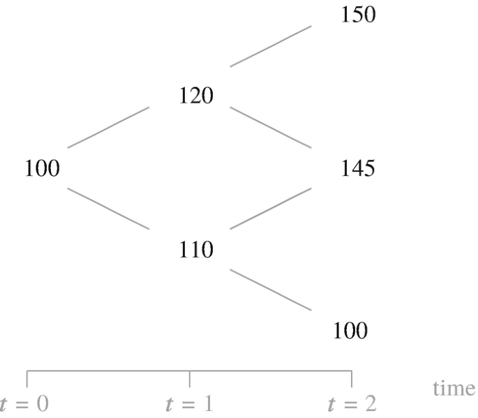

  

  Debt $\widetilde {D}_t$ of Problem 2

• 3. Prove that the tax shield $\widetilde {V}^l_t-\widetilde {V}^u_t$ satisfies

  $$\displaystyle \begin{aligned} \widetilde{V}^l_t-\widetilde{V}^u_t=\frac{\operatorname*{\mathrm{E}}_Q\left[\widetilde{V}^l_{t+1}-\widetilde{V}^u_{t+1}|\mathcal{F}_t\right]}{1+r_f}+\frac{\tau r_f\widetilde{D}_{t}}{1+r_f}\;. \end{aligned}$$

• 4. Prove that from (3.11) it follows that

  $$\displaystyle \begin{aligned} \widetilde{V}^l_t=\widetilde{V}^u_t+\tau\widetilde{D}_t+\sum_{s=t+1}^{T} \frac{\tau \operatorname*{\mathrm{E}}_Q\left[\widetilde{D}_{s}-\widetilde{D}_{s-1}|\mathcal{F}_t\right]}{(1+r_f)^{s-t}}\;. \end{aligned}$$

  This is the main result in Fernández (2005).

3.3 Autonomous Financing

3.3.1 Adjusted Present Value (APV)

When all future amounts of debt are already determined at valuation time t = 0, we are speaking of autonomous financing. In this case, the firm is following a completely fixed redemption plan. We are not really interested in whether or not autonomous financing is dealing with a realistic assumption. We, however, suppose that autonomous financing is pretty close to reality.

Definition 3.5 (Autonomous Financing)

A firm is autonomously financed exactly then when its future amount of debt $\widetilde {D}_t$ is already a certain quantity today.

Under this assumption, the tax advantages are also certain and can be discounted with the riskless rate. These leads straight to the so-called APV formula. The abbreviation stands for adjusted present value.

Theorem 3.6 (APV Formula)

In the case of autonomous financing, the following equation is valid for the market value of the levered firm at any time:

$$\displaystyle \begin{aligned} \widetilde{V}^l_t=\widetilde{V}^u_t+\sum_{s=t+1}^{T} \frac{\tau r_f D_{s-1}}{\left(1+r_f\right)^{s-t}}\;.\end{aligned} $$

This theorem can be proven as in the following. We work from the base of Eq. (3.11) and make use of the fact that our firm is following a fixed redemption policy. If the $\widetilde {D}_t$ are, however, no longer random variables, then the last equation is simplified on the basis of rule 3 to

$$\displaystyle \begin{aligned} \widetilde{V}^l_t=\widetilde{V}^u_t+\frac{\tau r_f D_{t}}{1+r_f}+\ldots +\frac{\tau r_f D_{T-1}}{\left(1+r_f\right)^{T-t}}\;.\end{aligned} $$

And that is how our theorem is proven.

Notice that our equation also holds for a firm with debt threatened by default! The value of the firm in danger of bankruptcy exactly corresponds to the value above, as long as the granted debt is certain. Although it can come to bankruptcy, the value of firms continues to be established by discounting the tax advantages from granted debt with the riskless interest rate and not the cost of debt or any other discount rate! What at first glance appears an unexpected result comes up because the creditors anticipate the threat of bankruptcy and therefore require interest payments, which perfectly compensate a possible loss of value due to bankruptcy.

Long-Term and Constant Amount of Debt

Finally, we want to look at the case where the amount of debt always remains the same. We then require that at time t the current debt will not change through redemption measures or further loans. In this case the last valuation formula can be simplified to an equation, which is named after those who discovered it.

Theorem 3.7 (Modigliani–Miller Formula)

If the firm goes on forever, the conditions of Theorem 3.6 are met and debt remains constant, then the following is valid for the market value of the levered firm

$$\displaystyle \begin{aligned} \widetilde{V}^l_t=\widetilde{V}^u_t+\tau D_{t}. \end{aligned}$$

To prove the theorem we convert the right summands in Theorem 3.6 with help of the geometric annuity. If debt remains constant we get

$$\displaystyle \begin{aligned} \widetilde{V}^l_t &=\widetilde{V}^u_t+\tau r_f D_{t}\sum_{s=t+1}^\infty \frac{1}{\left(1+r_f\right)^{s-t}}\\ &=\widetilde{V}^u_t+\tau r_f D_{t}\frac{1}{r_f}\;. \end{aligned} $$

And that is what we wanted to show.²²

We get a somewhat altered representation, if we concentrate on time t = 0 while supposing that the expected cash flows remain constant at that time. The amount of debt D₀ as the product of the debt ratio l₀ and market value of the levered firm can be written,

$$\displaystyle \begin{aligned} V^l_0&=V^u_0+\tau\,l_0\,V^l_0 \\ (1-\tau\,l_0) V^l_0 &= V^u_0. \end{aligned} $$

If we use the assumption that the expected free cash flows remain the same in time, then we can calculate the market value of the unlevered firm as cash value of a perpetual return, from which

$$\displaystyle \begin{aligned} \left(1-\tau\,l_0\right)V^l_0=\frac{\operatorname*{\mathrm{E}}\left[\widetilde{\mathit{FCF}}^u\right]}{k^{E,u}} \end{aligned}$$

and

$$\displaystyle \begin{aligned} V^l_0=\frac{\operatorname*{\mathrm{E}}\left[\widetilde{\mathit{FCF}}^u\right]}{(1-\tau\,l_0)k^{E,u}}\end{aligned} $$

follow. The last equation is also called Modigliani–Miller adjustment. The valuation equation proven in this chapter solves the problem as to how the market value is to be determined in full. We will come back to this equation once more in relation to the Miles–Ezzell adjustment.²³

Over-indebtedness and Illiquidity with Autonomous Financing

In the case of autonomous financing both default triggers can be precisely characterized. This is the main result of our next proposition where we assumed constant debt for simplicity.

Theorem 3.8 (Autonomous Financing)

A levered firm with an infinite life span whose amount of debt always remains the same is over-indebted in time t in state ω if and only if for its unlevered cash flows

$$\displaystyle \begin{aligned} \widetilde{\mathit{FCF}}^u_t(\omega)<\frac{(1-\tau)(k^{E,u}-g)}{1+g}\,\widetilde{D}.\end{aligned} $$

If the condition

$$\displaystyle \begin{aligned} \widetilde{\mathit{FCF}}^u_t(\omega)<r_f(1-\tau)\,\widetilde{D} \end{aligned}$$

is satisfied, the levered firm is in danger of illiquidity at date t in state ω.

Specifically, illiquidity (in state ω) implies over-indebtedness at time t (in the same state ω) if $g<\frac {k^{E,u}-r_f}{1+r_f}$.

Notice that the right-hand side of both inequalities is constant. If the cash flows of an unlevered company fall below this threshold, over-indebtedness occurs. The second inequality offers a more intuitive economic interpretation. If the cash flows go below the required interest payments after taxes, the firm is in danger of illiquidity.

The proof of the theorem is straightforward. The company is in danger of over-indebtedness if $\widetilde {V}^l_t(\omega ) < \widetilde {D}$ holds. For the financing policy considered here, $\widetilde {V}^l_t(\omega ) =\widetilde {V}^u_t(\omega )+\tau \widetilde {D}$ is valid. By plugging in, we see that

$$\displaystyle \begin{aligned} D > \frac{1}{1-\tau}\,\widetilde{V}^u_t(\omega)\end{aligned} $$

is true. Using Theorem 3.2 and solving for $\widetilde {\mathit {FCF}}^u_t(\omega )$ proves the proposition.

In order to prove the second statement we start with the fact that (due to constant debt) the firm is in danger of illiquidity if $\widetilde {\mathit {FCF}}^l_t(\omega )<r_f \widetilde {D}$ holds. Making use of the relationship between the free cash flows of a levered and those of an unlevered firm (3.10) and employing constant debt we get

$$\displaystyle \begin{aligned} \widetilde{\mathit{FCF}}^u_t(\omega)+\tau r_f \widetilde{D} &< r_f \widetilde{D}\end{aligned} $$

which proves the second statement.

3.3.2 Example (Continued)

The Finite Case Without Default

Here debt will be riskless, hence $\widetilde {k}^{D}_t=r_f$. If we suppose a future development of the amount of debt of

$$\displaystyle \begin{aligned} D_0=100,\quad D_1=100, \quad D_2=50\;, \end{aligned}$$

the value of the levered firm at time t = 0 is gotten with

$$\displaystyle \begin{aligned} \text{V}^l_0 &=\text{V}^u_0+\frac{\tau{r_f}D_0}{1+r_f}+\frac{\tau{r_f}D_1}{\left(1+r_f\right)^2}+\frac{\tau{r_f}D_2}{\left(1+r_f\right)^3} \\ &\approx 229.75+\frac{0.5\cdot 0.1\cdot 100}{1.1}+\frac{0.5\cdot 0.1\cdot 100}{1.1^2}+\frac{0.5\cdot 0.1\cdot 50}{1.1^3} \approx 240.30\;. \end{aligned} $$

The value of the levered firm is not essentially different from the value of the unlevered firm. That has to do with the fact that the firm in our example only has a lifetime of three years.

We deduced the market value of the levered firm at time t = 1 in an analogous way,

$$\displaystyle \begin{aligned} \widetilde{V}^l_1&=\widetilde{V}^u_1+\frac{\tau{r_f}D_1}{1+r_f}+\frac{\tau{r_f}D_2}{\left(1+r_f\right)^2} \\ &=\widetilde{V}^u_1+\frac{0.5\cdot 0.1\cdot 100}{1.1}+\frac{0.5\cdot 0.1\cdot 50}{1.1^2}\\ &\approx\begin{cases} 199.88, &\text{if the development in}\;t=1\;\text{is up,}\\ 164.74, &\text{if the development in}\;t=1\;\text{is down.}\\ \end{cases} \end{aligned} $$

Finally, we want to determine another additional outcome of our example. The levered firm’s debt ratio in regard to time t = 1 is an uncertain quantity. The following is valid:

$$\displaystyle \begin{aligned} \widetilde{l}_1\approx\begin{cases} \frac{100}{199.88} =50.03\%\,, &\text{if the development in}\;t=1\;\text{is up,}\\ \frac{100}{164.74} =60.70\%\,, &\text{if the development in}\;t=1\;\text{is down.}\\ \end{cases} \end{aligned}$$

If the firm is following an autonomous financing policy, it cannot be supposed that the debt ratio is certain. That is much more characteristic of financing based on market values.

Valuation in the Finite Case with Default Risk

It is not at all complicated to value the firm threatened with going into default in our example: we can use the APV formula. Therefore the value of the firm in danger of bankruptcy is calculated in our example by means of the Theorem 3.6 and exactly corresponds to the value above

$$\displaystyle \begin{aligned} \text{V}^l_0 \approx 240.30\;. \end{aligned}$$

Another way of obtaining this value of the firm would be to use the levered cash flows from Fig. 3.6, determine the expectations under Q and discount them with the riskless rate. This must yield just the same value.²⁴

An additional result, which, however, is not required for the valuation of the firm, is that for an amount of credit of D₂ = 50, we get at ω = dd a cost of debt of

$$\displaystyle \begin{aligned} \widetilde{k}^{D}_2(dd)&=\frac{\left(1+\widetilde{k}^{D,nom}_2(dd)\right)\,D_2\, P_3(u|dd)+\frac{1}{1-\tau}\left(\widetilde{\mathit{FCF}}^u_3(ddd)-\tau D_2\right) \, P_3(d|dd)}{D_2}-1\\ &\approx \frac{(1+0.32962)\cdot50\cdot 0.5+\frac{1}{1-0.5}\cdot(48.4-0.5\cdot 50)\cdot 0.5}{50}-1\\ & \approx 13.281\%. \end{aligned} $$

If the considerations employed above in relation to the nominal interest rates and their resultant cost of debt rates are systematically used again for other values of D₂, then for the interval D₂ ≤ 70, the relation depicted in Fig. 3.8 is gotten (see the Problem 5 below).

Fig. 3.8

Cost of debt and nominal interest rate with increasing leverage

The Infinite Case

Let the tax rate be τ = 50%. The levered firm maintains a debt schedule such that the amount of debt remains constant, D_t = 100. Debt is not threatened by default. As already indicated in the Modigliani–Miller formula the value of the levered firm is given by

$$\displaystyle \begin{aligned} V^l_0 &= V^u_0+\sum_{t=0}^\infty \frac{\tau{r_f}D_t}{\left(1+r_f\right)^{t+1}} \\ &=V^u_0+\tau D_0\\ &=500+0.5\cdot 100= 550\;. \end{aligned} $$

3.3.3 Problems

• 1. Let debt be riskless. Assume that the cash flows of the unlevered firm are weak auto-regressive. What assumptions on the debt schedule are necessary such that the cash flows of the levered firm $\widetilde {\mathit {FCF}}^l_t$ are weak auto-regressive as well?

• 2. Show that in the infinite example with constant (riskless) debt for all t

  $$\displaystyle \begin{aligned} \widetilde{V}^l_t=\frac{\widetilde{\mathit{FCF}}^u_t}{k^{E,u}}+\tau D_t. \end{aligned}$$

• 3. Show in the infinite example with constant (riskless) debt that the dividend-price ratio of the levered firm is a random variable (i.e., not deterministic) if r_f ≠ k^{E, u}.

• 4. Consider the finite example with default. Evaluate the Q-expected cash flows (see Fig. 3.6) and verify that the firm has indeed a value of 240.30.

• 5. Consider the finite example with default. Evaluate the cost of debt $\widetilde {k}^{D}_2$ as a function of debt D₂ ≤ 70.

3.4 Financing Based on Market Values

Let us turn our attention now to a further financing policy. In the following we will suppose that the managers of the firm to be valued are following a policy based on market values.

Definition 3.6 (Financing Based on Market Values)

A firm’s financing is based on market values exactly then when its debt ratios $\widetilde {l}_t$ are today already certain quantities.

A characterization of this financing in another context was that the firm’s leverage “breathes” with the equity’s market value. If the equity’s market value changes, then the amount of debt has to be adjusted.

Uncertain Tax Advantages

If a firm’s debt ratios and not its amount of debt are available, then autonomous financing is no longer the case. To illustrate the consequences, we suppose that management is aiming towards coming up with a debt ratio of 50:100, for instance, at a future time t > 0.²⁵ If we solve the debt ratio’s definition equation (3.5) according to $\widetilde {D}_t$, then with a deterministic ratio we get

$$\displaystyle \begin{aligned}l_t \widetilde{V}_t = \widetilde{D}_t.\end{aligned}$$

That means: If the value $\widetilde {V}_t$ is an uncertain quantity from today’s perspective, then the amount of debt relevant at this time is also stochastic, because the multiplication of a random variable by a real number results again in a random variable. Half of an uncertain quantity is of course also uncertain. In order to fully understand the relations, look at Fig. 3.9. With financing based on market values, the evaluator cannot say with certainty at time t = 0 how big the amount of debt will turn out to be at time t, since the value $\widetilde {V}_t$ is still uncertain and the amount of debt is firmly linked with this through the ratio. If this uncertainty is resolved—just a second after time t—then the interest payments to be rendered at time t + 1 are, in contrast, certain (if we neglect default for the moment). The same goes for the resulting tax savings $\tau \widetilde {\,I\,}_{t+1}$ at time t + 1. The tax savings is thus to be discounted with the riskless rate from time t + 1 to time t. But the discounting of t to 0 may not be carried out with r_f. It is uncertain from today’s perspective as to how much tax the firm proportionately financed by debt will save. Even with no default the discounting from t to 0 cannot be done with r_f. Today we cannot know how large the tax advantages from debt are.

Fig. 3.9

Time structure of financing based on market values

Miles and Ezzell (1980) have examined this case in detail and have determined that the APV equation of Theorem 3.6 is no longer suitable. The tax savings per terms of credit are uncertain and uncertain tax savings may not be discounted with the riskless rate.²⁶

Three Calculation Procedures

In the case of such a leverage policy, there are three different calculation procedures, which all lead to the same value of the firm. This value must differ from the value that would be calculated with the APV equation, since it is not based on an autonomous financing policy.

Which of the three calculations should be used by the evaluator depends upon, among other things, the state of information that she has on hand. We point out here that the content of the three equations which we have to prove is independent of financing based on market values: a policy based on market values is not absolutely necessary in all cases. Somewhat weaker conditions are instead enough: What is always important is that particular cost of capital are deterministic. To make this relation—which does at first glance seem complicated—understandable, we will first present the three formulations as generally as possible. At the end we will then show how they interrelate. It is not until this second step that the assumption of financing based on market values (and the fact that free cash flows of the unlevered firm are weak auto-regressive) will be made use of.

3.4.1 Flow to Equity (FTE)

In this section we will work with the assumption that the levered firm’s cost of equity is deterministic. In order to do so we must define the cost of equity. It is recommended to start off with determining the refluxes, which the equity financiers of the levered firm are entitled to. The starting quantities are the free cash flows of the indebted firm $\widetilde {\mathit {FCF}}^l_{t+1}$.

We have to deduct the payments to the creditors. These are entitled to interest as well as debt repayments at time t + 1. The interest claims amount to $\widetilde {\,I\,}_{t+1}$. We can evaluate the debt service as the difference between the paying back of former debt and the current value of debt, thus as $\widetilde {R}_{t+1}$. Altogether, the creditors are entitled payments in the amount of

$$\displaystyle \begin{aligned} \widetilde{\,I\,}_{t+1}+\widetilde{R}_{t+1} . \end{aligned}$$

If this is deducted from the starting amount, there then remains a residual amount for the owners (value of equity plus a dividend) of

$$\displaystyle \begin{aligned} \widetilde{E}_{t+1}+\widetilde{Div}_{t+1}:=\widetilde{E}_{t+1}+\widetilde{\mathit{FCF}}^l_{t+1} - \widetilde{\,I\,}_{t+1} - \widetilde{R}_{t+1}. \end{aligned} $$

(3.22)

This makes it clear as to how the definition of the cost of equity should read.

Definition 3.7 (Cost of Equity of the Levered firm)

The cost of equity $\,\widetilde {k}^{E,l}_t$ of a levered firm are conditional expected returns

$$\displaystyle \begin{aligned}\widetilde{k}^{E,l}_t:=\frac{\operatorname*{\mathrm{E}}\left[\widetilde{E}_{t+1}+ \widetilde{\mathit{FCF}}^l_{t+1} - \widetilde{\,I\,}_{t+1} -\widetilde{R}_{t+1} |\mathcal{F}_t\right]}{\widetilde{E}_t}-1. \end{aligned}$$

The index E with the cost of capital indicates that the cost of equity is being dealt with.

We now require that this cost of equity is deterministic. If we were to carry this assumption over to an actual firm listed on the exchange, it would entail being able to determine a firm’s future (conditional) expected returns on shares. We are fully aware that this condition is very rough. But it would be underhanded if we did not lay bare the implications of the assumptions, which form the basis of the various theories on discounted cash flow.

The valuation equation, which we now get is termed flow to equity (FTE), or also equity approach, in the literature. The reason flow to equity is spoken of is that the entire cash flows after taxes are not discounted, but rather those cash flows after taxes which the firm’s owners are entitled to.

Theorem 3.9 (Flow to Equity)

If the cost of equity of the levered firm $k^{E,l}_t$ are deterministic, then the value of equity at time t is

$$\displaystyle \begin{aligned} \widetilde{E}_t=\sum_{s=t+1}^T \frac{\operatorname*{\mathrm{E}}\left[ \widetilde{\mathit{FCF}}^l_{s}-\widetilde{\,I\,}_{s}-\widetilde{R}_{s} |\mathcal{F}_t\right]} {\left(1+k^{E,l}_{t}\right)\ldots\left(1+k^{E,l}_{s-1}\right)}. \end{aligned}$$

We have already used the method of proof required.²⁷ We can thus spare our readers it here.

3.4.2 Total Cash Flow (TCF)

If it is supposed that instead of the levered firm’s cost of equity the firm’s average cost of capital is deterministic, then it is the TCF approach and not the FTE approach which is being dealt with.

First the cost of capital which is now relevant has to be defined again. Which payments do the financiers of the levered firm receive? The answer is easily given. It is of course the free cash flows of the levered firm $\widetilde {\mathit {FCF}}^l_t$ that are the subject here. The capital employment of both groups of financiers is $\widetilde {E}_t+\widetilde {D}_t=\widetilde {V}^l_t$, so that the definition of the cost of capital for the case we now have to look at is absolutely clear.

Definition 3.8 (Weighted Average Cost of Capital—Type 1)

The weighted average cost of capital $\widetilde {k}^{\varnothing }_t$ of a levered firm are the conditional expected returns

$$\displaystyle \begin{aligned}\widetilde{k}^{\varnothing}_t:=\frac{\operatorname*{\mathrm{E}}\left[\widetilde{V}^l_{t+1}+\widetilde{\mathit{FCF}}^l_{t+1}|\mathcal{F}_t\right]}{\widetilde{V}^l_t}-1. \end{aligned}$$

How close to reality is the assumption of deterministic weighted average cost of capital? If we take a firm listed on the stock exchange for instance, then this condition calls for a knowledge of the entire future returns of the firm. A knowledge is needed thus not of the shares, or the (conditional) expectation of the returns on debt, but rather of the weighted average of both random quantities. A totally different assumption is being dealt with here than that condition on which the FTE formulation is based. We will be able to find out somewhat later if and in how far both conditions are compatible.

If we want to know, which value the levered firm has at time t, we can find the answer analogous to Theorem 2.1. The case being looked at here is termed total cash flow formulation (TCF), because the entire expected cash flows after taxes are discounted with the weighted average cost of capital.

Theorem 3.10 (Total Cash Flow)

If the weighted average cost of capital $k^{\varnothing }_t$ are deterministic, then the value of the firm at time t comes to

$$\displaystyle \begin{aligned} \widetilde{V}^l_t=\sum_{s=t+1}^T\frac{\operatorname*{\mathrm{E}}\left[\widetilde{\mathit{FCF}}^l_{s}|\mathcal{F}_t\right]} {\left(1+k^{\varnothing}_{t}\right)\ldots\left(1+k^{\varnothing}_{s-1}\right)} . \end{aligned}$$

A formal proof could be carried out again just as in Sect. 2.3.3, which is why we forgo with presenting it here again.

What can we say about the weighted average cost of capital (of type 1) and the cost of equity of a levered firm? Can we, for instance, ascertain that deterministic cost of equity also results from deterministic average cost of capital? Are then the FTE and TCF formulations compatible with each other? Or do both assumptions mutually exclude each other? Answers to all these questions are gotten by the so-called textbook formula.

Theorem 3.11 (TCF Textbook Formula)

For the type 1 weighted average cost of capital of the firm, the following relation is always valid:

$$\displaystyle \begin{aligned} \widetilde{k}^{\varnothing}_t=\widetilde{k}^{E,l}_t \, \left(1-\widetilde{l}_t\right)+\widetilde{k}^{D}_t\, \widetilde{l}_t. \end{aligned}$$

It is just now that it becomes really clear why weighted average cost of capital is spoken of in relation with the TCF formulation. The levered firm’s cost of equity is weighted with the equity ratio, and the cost of debt with the debt ratio.

To prove the theorem, we use the definition of the levered firm’s cost of equity. And after a few simplifications, we get

$$\displaystyle \begin{aligned} \left(1+\widetilde{k}^{E,l}_t\right)\widetilde{E}_t=\operatorname*{\mathrm{E}} \left[\widetilde{E}_{t+1}+ \widetilde{\mathit{FCF}}^l_{t+1}-\widetilde{\,I\,}_{t+1}-\widetilde{R}_{t+1} |\mathcal{F}_t \right]. \end{aligned}$$

Since the firm’s total value corresponds to the sum of equity and debt, you can apply according to rule 5 and under use of the Definitions 3.4, 3.7, and 3.8, the following:

$$\displaystyle \begin{aligned} \left(1+\widetilde{k}^{E,l}_t\right)\widetilde{E}_t+\left(1+\widetilde{k}^{D}_t\right)\widetilde{D}_t & = \operatorname*{\mathrm{E}}\left[\widetilde{V}^l_{t+1}+ \widetilde{\mathit{FCF}}^l_{t+1} |\mathcal{F}_t\right] \\ \widetilde{V}^l_t + \widetilde{k}^{E,l}_t \widetilde{E}_t + \widetilde{k}^{D}_t\widetilde{D}_{t} & = \left(1+\widetilde{k}^{\varnothing}_t\right) \widetilde{V}^l_t . \end{aligned} $$

After dividing by the firm’s market value, you come up with

$$\displaystyle \begin{aligned} 1+\widetilde{k}^{E,l}_t\frac{\widetilde{E}_t}{\widetilde{V}^l_t}+\widetilde{k}^{D}_t\frac{\widetilde{D}_t}{\widetilde{V}^l_t}=\widetilde{k}^{\varnothing}_t+1. \end{aligned}$$

Such is the assertion.

The textbook formula as it appears in Theorem 3.11 is remarkable in several aspects. To begin with, it is striking that it is obviously valid regardless of whether the relevant variables are understood as random variables or as deterministic quantities. Neither the weighted average cost of capital (type 1) nor the cost of equity of the levered firm (both a prerequisite of the FTE and the TCF approach) need to be deterministic in order to prove the textbook formula. A closer look at the textbook formula allows us to make the following determinations:

• 1. If it is assumed that the levered firm’s weighted average cost of capital (type 1) as well as cost of equity and debt are certain, then the debt ratios must also be certain.

  That is a big limitation, which cannot simply be accepted. But if we are working on the basis of certain debt ratios, then the textbook formula shows how the different cost of capital involved can be converted into each other. TCF and FTE may alternatively be used and inevitably lead to the same result.

• 2. If, on the other hand, in the case of no default the future debt ratios are seen as uncertain, either the weighted average cost of capital (type 1), or the cost of equity of the levered firm have to be uncertain.

  If the weighted average cost of capital (type 1) is deterministic, then the TCF concept has to be used; but if, on the other hand, the cost of equity is certain, then the FTE formulation has to be put into use, since uncertain cost of capital simply cannot be used to discount with. It does not make sense to pose the question here as to whether TCF and FTE methods lead to the same result. The textbook formula has no practical value in the case of uncertain debt ratios.

What further stands out with the textbook formula as it appears in Theorem 3.11 is that it is different from the usual textbook formula as it is given in relation to the weighted cost of capital (WACC) concept. In the former, the cost of debt cannot be reduced to the firm’s profit tax rate. We now want to discuss the question as to whether this cost of capital that is found in the literature also makes economic sense or whether it puts forth totally useless quantities.

3.4.3 Weighted Average Cost of Capital (WACC)

Look at the Definition 3.8 of the weighted average cost of capital. We now want to alter a very insignificant detail of this definition and call the resulting quantities WACC (weighted average cost of capital). The unlevered firm’s free cash flows take the place of the levered firm’s free cash flows.

Definition 3.9 (Weighted Average Cost of Capital—Type 2)

The cost of capital $\widetilde {WACC}$ of a levered firm are the expected returns

$$\displaystyle \begin{aligned} \widetilde{WACC}_t:=\frac{\operatorname*{\mathrm{E}}\left[\widetilde{V}^l_{t+1}+\widetilde{\mathit{FCF}}^u_{t+1}|\mathcal{F}_t\right]}{\widetilde{V}^l_t}-1. \end{aligned}$$

If these cost of capital is deterministic, we can again prove the existence of a valuation equation analogous to our previous approach. Beforehand, however, we want to discuss the question as to how realistic the assumption is that such cost of capital is observed on the market.

Whoever wants to establish the cost of capital in the sense of Definition 3.9, would have to look at a firm, which is on the one hand levered $\left (\widetilde {V}^l_t\right )$, and on the other pays free cash flows in an amount as if it were not levered, $\widetilde {\mathit {FCF}}^u_t$. It is clear that apples and oranges are being mixed here, and thus we may assume that no one can a priori know such cost of capital. We think that every other assertion would be senseless.

If we just momentarily free ourselves from this observation and the shackles it would enchain us in, then we could still formulate a valuation equation on the basis of this—albeit somewhat odd – definition of cost of capital. It would read as follows:

Theorem 3.12 (Weighted Average Cost of Capital)

If the levered firm’s cost of capital WACC _t are deterministic, then the value at time t of the firm financed by debt comes to

$$\displaystyle \begin{aligned} \widetilde{V}^l_t=\sum_{s=t+1}^T\frac{\operatorname*{\mathrm{E}}\left[\widetilde{\mathit{FCF}}^u_{s}|\mathcal{F}_t\right]} {\left(1+WACC_{t}\right)\ldots\left(1+WACC_{s-1}\right)} . \end{aligned}$$

The proof shows a clear course.

Critical readers will ask why we waste so much time on a cost of capital definition about which we have said that it makes no economic sense. The reason lies in the fact that this cost of capital definition—the direct interpretation of which makes no sense—will prove itself to be extremely useful in the following.

Theorem 3.13 (WACC Textbook Formula)

For the firm’s type 2 weighted average cost of capital, the following relation is always valid:

$$\displaystyle \begin{aligned} \widetilde{WACC}_t=\widetilde{k}^{E,l}_t \, \left(1-\widetilde{l}_t\right)+\widetilde{k}^{D}_t\,(1-\tau)\, \widetilde{l}_t. \end{aligned}$$

The WACC textbook formula is different from the TCF textbook formula only in that the interest on debt is reduced by the tax rate. That corresponds to the usual textbook formula given in the literature. Then the weighted average cost of capital results in that the cost of equity of the levered firm $\widetilde {k}^{E,l}_t$ is weighted with the equity ratio and the cost of debt—reduced by the firm’s income tax rate—with the debt ratio. Our calculation proves that this relation is valid independent of whether cost of equity and the debt ratio are certain or uncertain.

In order to prove the theorem we give the Definition 3.9 of the firm’s cost of equity using (3.14) in the form

$$\displaystyle \begin{aligned}\left(1+\widetilde{WACC}_t\right) \widetilde{V}^l_t = \operatorname*{\mathrm{E}}\left[\widetilde{E}_{t+1}+\widetilde{D}_{t+1}+\widetilde{\mathit{FCF}}^l_{t+1}-\tau\left(\widetilde{\,I\,}_{t+1}+ \widetilde{R}_{t+1}+\widetilde{D}_{t+1}-\widetilde{D}_t\right)|\mathcal{F}_t\right].\end{aligned}$$

From taking advantage of Definitions 3.4 and 3.7 we get

$$\displaystyle \begin{aligned} \left(1+\widetilde{WACC}_t\right) \widetilde{V}^l_t &= \operatorname*{\mathrm{E}}\left[\widetilde{E}_{t+1}+\widetilde{\mathit{FCF}}^l_{t+1}-\widetilde{\,I\,}_{t+1}-\widetilde{R}_{t+1}+\right.\\ &\left.\qquad +(1-\tau)\left(\widetilde{D}_{t+1}+\widetilde{\,I\,}_{t+1}+\widetilde{R}_{t+1}\right)-\tau\widetilde{D}_t|\mathcal{F}_t\right]\\ &= \left(1+k^{E,l}_t\right)\widetilde{E}_t+\left(\left(1+\widetilde{k}^{D}_t\right)(1-\tau)+\tau\right)\widetilde{D}_t . \end{aligned} $$

Divided by $\widetilde {V}^l_t$ and observing Definition 3.5, we finally get to the following representation:

$$\displaystyle \begin{aligned} \widetilde{WACC}_t = \widetilde{k}^{E,l}_t \left(1-\widetilde{\widetilde{l}}_t\right) + \widetilde{k}^{D}_t(1-\tau)\widetilde{l}_t. \end{aligned}$$

And that is what we wanted to show.

This textbook formula also allows for the following conclusions.

• 1. If it is assumed that the weighted average cost of capital as well as the cost of equity and debt of the levered firm are certain today, then the debt ratios must be certain. We are then dealing with a financing policy based on market values. FTE and WACC result in identical values of the firm in this case.

• 2. If the future debt ratios are, however, assumed to be uncertain, then in the case of no default either the weighted average cost of capital, or the cost of equity of the levered firm have to be uncertain. Thus one of the two theorem’s formulations cannot be used to calculate with.

We want to summarize our statements made up to now on financing based on market values in Fig. 3.10. The illustration makes clear that the three procedures FTE, TCF, and WACC result in an identical value of the firm exactly then when the debt ratio is deterministic. In all other cases, only one of the three procedures can be used at most.

Fig. 3.10

DCF theory for financing based on market value

The attentive reader will notice that in all statements in this and the former section we have not made use of our assumption that the cash flows are weak auto-regressive. We now turn to the adjustment formulas where this assumption will be necessary.

3.4.4 Miles–Ezzell- and Modigliani–Miller Adjustments

In the previous sections we got three different valuation equations for a levered firm with financing based on market values: FTE, TCF, and WACC formulas. We could clearly work out that these valuation equations can always typically be used when either the levered firm’s cost of equity or the weighted average cost of capital (from type 1 or 2) is deterministic. We could make connections between the different cost of capital relevant for the three formulations with the so-called textbook formulas. Financing policy based on value stands out in that the debt ratios are deterministic. Our analysis of the textbook formulas established that with this type of financing policy, deterministic cost of capital of the two remaining valuation formulations logically results from deterministic cost of capital of a valuation formulation.

Until now, however, the relationship these three cost of capital demonstrate to the cost of capital of an unlevered firm has remained a secret. And exactly that is the subject of our subsequent considerations. If we require that the levered firm follows a financing policy based on market values, and if in addition we assume that the cost of equity of the unlevered firm are deterministic, then two questions arise:

• 1. Under these conditions, are the requirements of Theorems 3.9 and 3.12 met? Are the levered firm’s cost of equity and the weighted average cost of capital then also deterministic?

• 2. Can we calculate the levered firm’s cost of capital from the unlevered firm’s cost of capital?

Adjustment According to Miles and Ezzell

The answer to both questions is given by the so-called adjustment formula from Miles and Ezzell (1980).

Theorem 3.14 (Miles–Ezzell Adjustment Formula)

Financing based on market values is under consideration. The cash flows of the unlevered firm are weak auto-regressive. If the unlevered firm’s cost of capital or the WACC of the levered firm are deterministic, the following relation is valid:

$$\displaystyle \begin{aligned} 1+WACC_t=\left(1+k^{E,u}_t\right)\left(1-\frac{\tau r_f}{1+r_f}\,l_t\right), \end{aligned}$$

in which all quantities in the equation are deterministic.

We prove this theorem as follows. According to the fundamental theorem and using Eq. (3.14), the following is valid for the market value: of the levered firm

$$\displaystyle \begin{aligned} \widetilde{V}^l_t=\frac{\operatorname*{\mathrm{E}}_Q\left[\widetilde{V}^l_{t+1}+\widetilde{\mathit{FCF}}^u_{t+1}+\tau\left( \widetilde{\,I\,}_{t+1}+\widetilde{R}_{t+1}+\widetilde{D}_{t+1}-\widetilde{D}_t\right)|\mathcal{F}_t\right]}{1+r_f}\,. \end{aligned}$$

Since the market value of the firm at time t is already known, the following results from rules 2 and 5 and Eq. (3.19):

$$\displaystyle \begin{aligned} \widetilde{V}^l_t=\frac{\operatorname*{\mathrm{E}}_Q\left[\widetilde{V}^l_{t+1}+\widetilde{\mathit{FCF}}^u_{t+1}|\mathcal{F}_t\right]}{1+r_f}+\frac{\tau r_f }{1+r_f}\,\widetilde{D}_{t}. \end{aligned}$$

Using the debt ratio, this can be rewritten in the form

$$\displaystyle \begin{aligned} \left(1-\frac{\tau r_f }{1+r_f}\,l_t\right)\widetilde{V}^l_t=\frac{\operatorname*{\mathrm{E}}_Q\left[\widetilde{V}^l_{t+1}+\widetilde{\mathit{FCF}}^u_{t+1}|\mathcal{F}_t\right]}{1+r_f} \end{aligned}$$

or

$$\displaystyle \begin{aligned} \widetilde{V}^l_t=\frac{\operatorname*{\mathrm{E}}_Q\left[\widetilde{V}^l_{t+1}+\widetilde{\mathit{FCF}}^u_{t+1}|\mathcal{F}_t\right]}{\left(1-\frac{\tau r_f }{1+r_f}\,l_t\right)\left(1+r_f\right)}\;. \end{aligned}$$

We are then looking at a type of recursive relationship from which we have already gotten a valuation equation several times.²⁸ Following this direction, we get this relation for the value of the levered firm

$$\displaystyle \begin{aligned} \widetilde{V}^l_t=\sum_{s=t+1}^T\frac{\operatorname*{\mathrm{E}}_Q\left[\widetilde{\mathit{FCF}}^u_{s}|\mathcal{F}_t\right]}{\left(1-\frac{\tau r_f }{1+r_f}\,l_{s-1}\right)\ldots\left(1-\frac{\tau r_f }{1+r_f}\,l_{t}\right)\left(1+r_f\right)^{s-t}}\;. \end{aligned}$$

Now we will only get further by falling back upon the Assumption 3.1 and the Theorem 3.3 supported by it.²⁹ If we use this theorem, we get

$$\displaystyle \begin{aligned} \widetilde{V}^l_t=\sum_{s=t+1}^T\frac{\operatorname*{\mathrm{E}}\left[\widetilde{\mathit{FCF}}^u_{s}|\mathcal{F}_t\right]}{\left(1-\frac{\tau r_f }{1+r_f}\,l_{t}\right)\left(1+k^{E,u}_{t}\right)\ldots\left(1-\frac{\tau r_f }{1+r_f}\,l_{s-1}\right)\left(1+k^{E,u}_{s-1}\right)}\;. \end{aligned}$$

From that now results the recursive relation

$$\displaystyle \begin{aligned} \widetilde{V}^l_t=\frac{\operatorname*{\mathrm{E}}\left[\widetilde{V}^l_{t+1}+\widetilde{\mathit{FCF}}^u_{t+1}|\mathcal{F}_t\right]}{\left(1-\frac{\tau r_f }{1+r_f}\,l_t\right)\left(1+k^{E,u}_t\right)} \end{aligned}$$

or

$$\displaystyle \begin{aligned} \left(1-\frac{\tau r_f }{1+r_f}\,l_t\right)\left(1+k^{E,u}_t\right)=\frac{\operatorname*{\mathrm{E}}\left[\widetilde{V}^l_{t+1}+\widetilde{\mathit{FCF}}^u_{t+1}|\mathcal{F}_t\right]}{\widetilde{V}^l_t}\;. \end{aligned}$$

A comparison with the Definition 3.9 shows that we have proven the claim.

If the equation from Theorem 3.14 is linked up with the textbook formula from Theorem 3.13, the meaning of the outcome becomes much clearer. Putting the textbook formula into the equation of Theorem 3.14 and slightly reworking it results in

$$\displaystyle \begin{aligned} k^{E,l}_t=k^{E,u}_t+L_t\left(k^{E,u}_t-k^{D}_t+\tau\left(k^{D}_t-\frac{1+k^{E,u}_t}{1+r_f}\,r_f\right)\right), \end{aligned} $$

(3.23)

in which L_t represents the debt-equity ratio in the sense of Eq. (3.6). The cost of capital of the levered firm can be determined with this formula, if the cost of capital of the unlevered firm, the cost of debt, the income tax rate as well as the aspired leverage ratio and the riskless interest rate are known. If the above equation is solved according to $k^{E,u}_t$, the leverage ratio, and income tax rate are known, it calls for converting the cost of capital of a levered firm into the cost of capital of the unlevered firm. The condition is that the levered firm follows a financing policy based on market values.

The reader may want to take the time and take another look at Eq. (3.23). It is different in two not so unimportant details which are found in the original theorem from Miles and Ezzell (1980). We want to mention these differences with absolute clarity as the work from Miles and Ezzell has firmly established itself in today’s textbook literature. With their formula there is no time index for the leverage ratio and also no time index for the cost of capital. In the current literature then, the adjustment formula does not run as it does in our Theorem 3.14, but rather

$$\displaystyle \begin{aligned} 1+WACC=\left(1+k^{E,u}\right)\left(1-\frac{\tau r_f}{1+r_f}\,l\right) . \end{aligned} $$

(3.24)

Miles and Ezzell derived their result under the limitation of the assumption that the cost of capital and the debt ratio are constant in time. As a rule, this limitation is clearly pointed out in the textbook literature. The outcome that we have shown thus has much fewer restrictions than the original result from Miles and Ezzell.

Second, our adjustment formula also holds in case of a firm in danger of default. Even though the firm can go bankrupt, still not the cost of debt or any other discount factor but the riskless interest rate is found in Theorem 3.14. This is a surprising, but an inescapable consequence of our assumptions, that not only the owners, but also the creditors anticipate the threat of bankruptcy.

Problematic Adjustment According to Modigliani and Miller

In the discussion of autonomous financing, we had mentioned that besides the Miles–Ezzell adjustment, there is yet another adjustment formula. It is termed Modigliani–Miller adjustment, originates from Theorem 3.7 and takes the form

$$\displaystyle \begin{aligned} WACC = k^{E,u} (1-\tau l_0). \end{aligned} $$

(3.25)

In practice, this adjustment formula is very popular, supposedly because it looks much more simple than the Miles–Ezzell equation (3.24). If you follow the relevant literature, then you get Eq. (3.25) from the conditions of Theorem 3.7 and particularly from the assumption of autonomous financing. Such a firm then cannot be financed based on market values. We will now present a surprising outcome.

Theorem 3.15 (Contradiction of the Modigliani–Miller Adjustment)

The cash flows of the unlevered firm are weak auto-regressive. If the weighted average cost of capital of type 2 (WACC) and the unlevered firm’s cost of equity (k ^E,u ) are deterministic, then the firm is financed based on market values.

First off we will prove the theorem and end up trying to recognize its significance. To prove the theorem we turn to the Theorems 3.1, 3.7, and 3.12 and use the fact that cash flows are weak auto-regressive. The following then applies:

$$\displaystyle \begin{aligned} \begin{array}{rcl} &\displaystyle &\displaystyle \left(1-\tau \widetilde{l}_t\right)\underbrace{\sum_{s=t+1}^T \frac{(1+g_{t})\ldots (1+g_{s-1})\widetilde{\mathit{FCF}}^u_t}{\left(1+WACC_t\right)\ldots (1+WACC_{s-1})}}_{= \widetilde{V}_t^l}= \\&\displaystyle &\displaystyle \qquad \qquad \qquad \qquad \qquad \qquad \qquad \quad =\underbrace{\sum_{s=t+1}^T \frac{(1+g_{t})\ldots(1+g_{s-1})\widetilde{\mathit{FCF}}^u_t}{\left(1+k^{E,u}_t \right)\ldots\left(1+k^{E,u}_{s-1}\right)}}_{=\widetilde{V}_t^u}. \end{array} \end{aligned} $$

If we shorten $\widetilde {\mathit {FCF}}^u_t$, there remains

$$\displaystyle \begin{aligned} \begin{array}{rcl} &\displaystyle &\displaystyle \left(1-\tau \widetilde{l}_t\right)\sum_{s=t+1}^T \frac{(1+g_{t})\ldots(1+g_{s-1})}{(1+WACC_t)\ldots(1+WACC_{s-1})}= \\&\displaystyle &\displaystyle \qquad \qquad \qquad \qquad \qquad \qquad \qquad \quad =\sum_{s=t+1}^T \frac{(1+g_{t})\ldots(1+g_{s-1})}{\left(1+k^{E,u}_t\right) \ldots\left(1+k^{E,u}_{s-1}\right)}. \end{array} \end{aligned} $$

Besides the debt ratio $\widetilde {l}_t$ we only find deterministic quantities. It is no problem to convert them according to $\widetilde {l}_t$. But then $\widetilde {l}_t$ has to be a deterministic quantity itself. That is what we wanted to show.

Of what significance is our assertion now? A Modigliani–Miller adjustment formulated as in Eq. (3.25) requires that the weighted average cost of capital as well as the equity of the unlevered firm are deterministic. The equation does not make sense under other conditions. Under this condition—we have just proven this—the case of financing based on market values is now indeed conceivable. And here is where the anomaly lies: the condition of the Modigliani–Miller model was, namely, autonomous financing with constant debt. Since a firm cannot be financed autonomously as well as based on market values, we have a contradiction. We do not object that there will be real numbers WACC that (in the case of autonomous financing) lead to the correct value of the levered firm. These numbers are appropriate discount rates given the above setup—but they cannot be interpreted as cost of capital as in Definition 3.9. This again highlights that cost of capital and discount rates cover different economic items.

Can we go a step further and claim to have refuted the theory of Modigliani and Miller? Have we perhaps detected an error in the argumentation of both authors? In answering this question, we have to carefully separate two aspects from each other. In this book we take the point of view that cost of capital are expected returns. For us that is the nucleus of a theory of valuation of firms. If this line of thought is followed, then the ideas of Modigliani and Miller simply do not hold up. Whoever interprets WACC as expected returns, cannot simultaneously suppose a deterministic debt ratio and the Modigliani–Miller model (a constant amount of debt), without getting caught in a contradiction. To come at it from a totally different angle, we can ask if Modigliani and Miller had even understood WACC as cost of capital and been aware of the contradiction. The answer here is unambiguous. For both authors—as, moreover, also for Miles and Ezzell—the weighted cost of capital WACC was always only a quantity, which when used as a discount rate leads to the correct outcome; that is, the correct value of the firm.³⁰ Not one of these authors thought of an interpretation of these quantities as expected returns. This is why we are far away from blaming Modigliani and Miller for making an error.

3.4.5 Over-Indebtedness and Illiquidity with Financing Based on Market Values

We now turn to the case of financing based on market values. Here, the case of over-indebtedness will never occur. Illiquidity is possible and a sufficient condition can be precisely formulated.

Theorem 3.16 (Over-Indebtedness and Debt Ratio)

A levered firm with an infinite life span whose debt ratio l always remains the same is never over-indebted.

If the condition

$$\displaystyle \begin{aligned} \frac{\widetilde{\mathit{FCF}}^u_t(\omega)}{\widetilde{\mathit{FCF}}^u_{t-1}(\omega)} < \frac{(1+r_f(1-\tau)) (1+g)}{1+ \frac{k^{E,u}-g}{l}-\frac{1+k^{E,u}}{1+r_f}r_f\tau +g} \end{aligned}$$

is satisfied, then the firm is in danger of illiquidity at date t in state ω.

Again, the implications of this proposition can be illustrated by means of a binomial tree with only the case of illiquidity being of interest. The second part of the theorem requires that the growth factor for the down-movement (the left-hand side of the inequality) must not fall below a specific threshold.

The first statement of the theorem can easily be proven because for l ≤ 1 we obtain $l\;\widetilde {V}^l_t(s) \le \widetilde {V}^l_t(s)$ and thus $\widetilde {D}_t (s)\le \widetilde {V}^l_t(s)$. The proof of the second statement is more sophisticated. Let us assume that the firm always remains liquid. In this case

$$\displaystyle \begin{aligned} \widetilde{\mathit{FCF}}^l_t(\omega) \ge (1+r_f) \widetilde{D}_{t-1}(\omega)-\widetilde{D}_t(\omega) . \end{aligned}$$

To refer to the unlevered firm’s cash flows, we make use of Eq. (3.10) and obtain

$$\displaystyle \begin{aligned} \widetilde{\mathit{FCF}}^u_t(\omega) +\tau r_f \widetilde{D}_{t-1}(\omega)&\ge (1+r_f) \widetilde{D}_{t-1}(\omega)-\widetilde{D}_t(\omega) \\ \widetilde{\mathit{FCF}}^u_t(\omega) &\ge (1+r_f(1-\tau)) \widetilde{D}_{t-1}(\omega)-\widetilde{D}_t(\omega)\\ \widetilde{\mathit{FCF}}^u_t(\omega) &\ge (1+r_f(1-\tau)) l \widetilde{V}^l_{t-1}(\omega)-l \widetilde{V}^l_t(\omega). \end{aligned} $$

In the case of an eternally active firm with constant cost of capital, the firm value can be calculated by dividing the expected free cash flow by the cost of capital less the constant growth rate. For financing based on market values $\widetilde {V}^l_t(\omega )=\frac {(1+g) \widetilde {\mathit {FCF}}^u_t(\omega )}{WACC-g}$ suits. Therefore, we obtain a total of

$$\displaystyle \begin{aligned} \widetilde{\mathit{FCF}}^u_t(\omega) &\ge (1+r_f(1-\tau)) l \frac{(1+g) \widetilde{\mathit{FCF}}^u_{t-1}(\omega)}{WACC -g}-l \frac{(1+g)\widetilde{\mathit{FCF}}^u_{t}(s)}{WACC -g }\\ \left(1+\frac{l (1+g)}{WACC -g}\right)\widetilde{\mathit{FCF}}^u_t(\omega) &\ge (1+r_f(1-\tau)) l\frac{(1+g) \widetilde{\mathit{FCF}}^u_{t-1}(\omega)}{WACC -g } \end{aligned} $$

which proves the assertion.

3.4.6 Example (Continued)

The Finite Case Without Default

In our example the firm will be financed based on market values. In this case all three approaches FTE, TCF, and WACC will yield the same value of the firm. Since the leverage ratios are given, we concentrate on the WACC approach.

Now we suppose in contrast to the autonomous financing that the following capital structures are realized at future times:

$$\displaystyle \begin{aligned} l_0=50\%\,, \quad l_1=20\%\,, \quad l_2=0\%\,. \end{aligned}$$

The weighted average cost of capital results from the Miles–Ezzell equation with

$$\displaystyle \begin{aligned} WACC_0&=\left(1+k^{E,u}\right)\left(1-\frac{\tau r_f}{1+r_f}\,l_0\right)-1\\ &=\left(1+0.2\right)\left(1-\frac{0.5 \cdot 0.1}{1+0.1}\cdot 0.5\right)-1 \approx17.27\%\,, \\ WACC_1&\approx 18.91\% ,\\ WACC_2&=20\% . \end{aligned} $$

With that the value of the firm amounts to

$$\displaystyle \begin{aligned} V_0^l &= \frac{\operatorname*{\mathrm{E}}\left[\widetilde{\mathit{FCF}}^u_1\right]}{1+WACC_0}+ \frac{\operatorname*{\mathrm{E}}\left[\widetilde{\mathit{FCF}}^u_2\right]}{(1+WACC_0)(1+WACC_1)}\;+\\ &\qquad \qquad + \frac{\operatorname*{\mathrm{E}}\left[\widetilde{\mathit{FCF}}^u_3\right]}{(1+WACC_0)(1+WACC_1)(1+WACC_2)}\\ &\approx \frac{100}{1.1727}+ \frac{110}{1.1727 \cdot 1.1891}+ \frac{121}{1.1727 \cdot 1.1891 \cdot 1.20} \approx 236.46\;. \end{aligned} $$

Financing based on market values obviously leads to a totally different value of the firm than autonomous financing.

When considering default we need the value of the company at time t = 1. Here we get

$$\displaystyle \begin{aligned} \widetilde{V}^l_1&= \frac{\operatorname*{\mathrm{E}}\left[\widetilde{\mathit{FCF}}^u_2|\mathcal{F}_1\right]}{1+WACC_1}+ \frac{\operatorname*{\mathrm{E}}\left[\widetilde{\mathit{FCF}}^u_3|\mathcal{F}_1\right]}{(1+WACC_1)(1+WACC_2)}\\ &\approx\left\{\begin{array}{ll} \frac{121}{1.1891}+\frac{133.1}{1.1891\cdot 1.20}\approx 195.04, & \mbox{if up;} \\ \frac{99}{1.1891}+\frac{108.9}{1.1891\cdot 1.20}\approx 159.58, & \mbox{if down.} \end{array}\right. \end{aligned} $$

Due to the financing policy based on market values, the payments for the creditors shown in Fig. 3.11 will be yielded in the future. Please observe that l₂ = 0 applies.³¹

Fig. 3.11

Debtor’s claims if l₀ = 50% , l₁ = 20% , l₂ = 0%

The Finite Case with Default

Now we will go into the question as to if a finance based on market values can lead to bankruptcy and, if possible, complete our model in a suitable way. To this end we remind our reader that the provisional leverage policy is assumed to take the form

$$\displaystyle \begin{aligned} l_0=50\%\,,\quad l_1=20\%\,, \quad l_2=0\%\,.\end{aligned} $$

We want to evaluate the free cash flows $\widetilde {\mathit {FCF}}^l_t$ of the levered firm with default risk. Default enters in if

$$\displaystyle \begin{aligned} \widetilde{\mathit{FCF}}^l_t -\left(1+r_f\right)\, l_{t-1}\,\widetilde{V}^l_{t-1}+l_{t}\,\widetilde{V}^l_{t}<0\end{aligned} $$

is given. Again, we have systematically compiled the corresponding amounts in Fig. 3.12. The figure shows that at time t = 1 a problem comes up, the case of bankruptcy is at issue.

Fig. 3.12

Shareholder’s claims without default if l₀ = 50% , l₁ = 20% , l₂ = 0%

This generates an interruption of payments but does not cause an inability to pay. Therefore, in contrast to the situation in Sect. 3.2.6, the shareholders can avert a default. It is quite obvious that in t = 1 the credit D₀ as well as the owing interests r_fD₀ cannot be paid completely. A possible solution would be an extension for payment. Assuming that the creditors accept an extension for capital deficit of 2.23 until t = 2, a default would be prevented. But such a step disagrees with our assumptions: We assumed that the investors pursue an exogenous leverage policy even if it is not optimal. In our case, it is the described extension for credit which disagrees with the assumption. This example shows exactly the limitations of our model. If (and only if) the leverage policy is given, the default risk has no influence at all on the value of the company.

As a matter of course, in a situation such as shown in Fig. 3.12, the owners of the company will certainly demand a financing policy which is different from the one originally planned. It is obvious that a different financing policy leads to another company value. But we will not care about the question which financing policy would be the most reasonable. Even though the originally agreed financing policy could be evaluated, we state that this policy is economically illogical. Therefore, we will cease the discussion of our example.

The Infinite Case

Let us turn to the infinite case. We assume that the leverage ratio l = 50% remains constant. If we use the Miles–Ezzell adjustment (Theorem 3.14), the weighted average cost of capital are

$$\displaystyle \begin{aligned} WACC=(1+k^{E,u})\left(1-\frac{\tau r_f}{1+r_f}l\right)-1\approx 17.273\% \end{aligned}$$

and from Theorem 3.12 we get

$$\displaystyle \begin{aligned} V^l_0&=\sum_{t=1}^\infty \frac{\operatorname*{\mathrm{E}}\left[\widetilde{\mathit{FCF}}^u_t|\mathcal{F}_0\right]}{(1+WACC)^{t}}\\ &=\sum_{t=1}^\infty \frac{FCF^u_0}{(1+WACC)^{t}} =\frac{FCF^u_0}{WACC}\\&\approx \frac{100}{0.17273}\approx 578.947\;. \end{aligned} $$

This is the value of the levered firm at t = 0.

3.4.7 Problems

• 1. Consider a company having (unlevered) cash flows as in Fig. 2.2. The tax rate is 50% and the riskless interest rate 10%. Assume further that WACC = 18%, but nothing is known about the cost of equity k^{E, u}. We do not require that the company maintains a deterministic leverage ratio $\widetilde {l}$ and will show with this problem that the other DCF methods of this chapter are not applicable.

  • (a) Evaluate the value of the firm using the WACC method for t = 0, 1.

  • (b) Convince yourself that no assumptions are made yet about the expected future amount of debt since we do not require a deterministic leverage ratio. Instead, for t = 0, 1 we will assume the following debt: schedule

    $$\displaystyle \begin{aligned} D_0=50, \quad \widetilde{D}_1=\begin{cases} 60&\text{if up,}\\ 40&\text{if down.} \end{cases} \end{aligned}$$

    Determine the leverage ratio at t = 1 and show that the firm is not financed based on market values.

  • (c) Evaluate the weighted cost of capital (type 1) at t = 1 as well as the cost of equity of the levered firm and show that they both are random variables.

• 2. Show that for k^{E, u} > r_f the Miles–Ezzell-WACC from (3.24) is always larger than k^{E, u}(1 − τl₀) if l₀ = l is the leverage ratio of the firm.

• 3. Verify that in the infinite example

  $$\displaystyle \begin{aligned} \widetilde{V}^l_t=\frac{\widetilde{V}^u_t}{1-\frac{1+k^{E,u}}{1+r_f}\frac{r_f}{k^{E,u}}\tau l} . \end{aligned}$$

  (This is the main result of Miles and Ezzell (1985).)

• 4. Cost of capital are often evaluated using the capital asset pricing model (CAPM). Due to the CAPM any cost of capital k are given by

  $$\displaystyle \begin{aligned} k_t=r_f+\left(\operatorname*{\mathrm{E}}\left[r_M\right]-r_f\right) \, \beta_t, \end{aligned}$$

  where r_M is the return on the market portfolio and β_t the so-called beta factor. Let $\beta ^{WACC}_t$ be the beta factor of WACC_t and $\beta ^{E,u}_t$ of $k^{E,u}_t$. Write down a beta form of the Miles–Ezzell formula.

3.5 Financing Based on Book Values

Until now, we have debated two forms of financing policy, which are often discussed in the literature. With autonomous financing the taking out and redemption of debt followed a static, pre-given plan, which did not take any kind of random developments into consideration. With financing based on market values in contrast, the risk of debt was linked to the random development of the equity’s market value by a given relation. For firms listed on the exchange that means that with climbing share prices, loans are to be taken out, and that with falling prices, debts are to be redeemed. We have stressed again and again that we want to lay back on making claims about which of the different financing policies is particularly realistic. If we bring another financing policy into play in the following, it is because we have the impression that it most probably plays an important role in business practice. If the managers of a firm announce that they are planning on lowering or raising the leverage ratio, then they are usually not measuring the leverage ratio in market values, but in book values. Both value formulations widely diverge from each other. That motivates us to analyze a third financing policy in the following section. Just as financing based on market values, this is based on debt ratios; this time, however, as book values.

3.5.1 Assumptions

With debt and equity as book values, those amounts are in question with which the debts or—according to case—equity are reported in the balance books of the firm to be valued. The first assumption consists in there being no difference between market value and book value of the debt. The credit amounts given in the balance sheets of the firm to be valued correspond to their market prices. Furthermore, we will assume that there is no danger of default.

Assumption 3.7 (Book Value of Debt)

The firm will not default

$$\displaystyle \begin{aligned} \widetilde{R}_{t+1}=\widetilde{D}_t-\widetilde{D}_{t+1} \quad \mathit{\text{and}}\quad \widetilde{\,I\,}_{t+1}=r_f\widetilde{D}_t.\end{aligned} $$

Furthermore, the debt’s market value continuously corresponds to its book value,

$$\displaystyle \begin{aligned} \widetilde{\underline{D}}_t = \widetilde{D}_t . \end{aligned}$$

It is different with equity. If you are working from an initial quantity of $\widetilde { \underline {E}}_t$ and inquire about the book value of the equity at time t + 1, then you have to look at those quantities, which can change it. There are three:

• 1. Equity grows, if the owners subscribe additional equity within the framework of an increase of capital. The amount of the increase in capital between the times t and s is designated by $\widetilde { \underline {e}}^l_{t,s}$.³²

• 2. Equity grows further if the managers retain earnings. The levered firm’s earnings after taxes at time t + 1 amount to $\left ( \widetilde {EBIT}_{t+1} - \widetilde {\,I\,}_{t+1}\right ) (1-\tau )$.

• 3. Equity decreases if the firm pays dividends to the owners. In relation to the FTE approach and using Eq. (3.14), we made clear that payments in the amount of

  $$\displaystyle \begin{aligned}\widetilde{\mathit{FCF}}^u_{t+1} + \tau\widetilde{\,I\,}_{t+1}- \Big( \widetilde{\,I\,}_{t+1}+\widetilde{D}_{t} -\widetilde{D}_{t+1} \Big) \end{aligned}$$

  are being dealt with.³³

For the book value of the equity at time t + 1, we get a total of

$$\displaystyle \begin{aligned} \widetilde{\underline{E}}^l_{t+1} &= \widetilde{\underline{E}}^l_t + \widetilde{\underline{e}}^l_{t,t+1} + \left( \widetilde{EBIT}_{t+1} - \widetilde{\,I\,}_{t+1} \right) (1-\tau) \\ & \qquad - \left( \widetilde{\mathit{FCF}}^u_{t+1}+\tau\widetilde{\,I\,}_{t+1} - \Big( \widetilde{\,I\,}_{t+1}+\widetilde{D}_{t} - \widetilde{D}_{t+1} \Big) \right) \\ &= \widetilde{\underline{E}}^l_t + \widetilde{\underline{e}}^l_{t,t+1} + \widetilde{EBIT}_{t+1} (1-\tau) - \widetilde{\mathit{FCF}}^u_{t+1} + \widetilde{\underline{D}}_t - \widetilde{\underline{D}}_{t+1}. \end{aligned} $$

This gives nothing more than the clean surplus relation.

Assumption 3.8 (Clean Surplus Relation)

The book value of a levered firm results from

$$\displaystyle \begin{aligned} \widetilde{\underline{E}}^l_{t+1} = \widetilde{\underline{E}}^l_t + \widetilde{\underline{e}}^l_{t,t+1} + \widetilde{EBIT}_{t+1} (1-\tau) - \widetilde{\mathit{FCF}}^u_{t+1} + \widetilde{\underline{D}}_t - \widetilde{\underline{D}}_{t+1}. \end{aligned}$$

Since $\widetilde { \underline {V}}_{t}=\widetilde { \underline {E}}^l_{t}+\widetilde { \underline {D}}_{t}$, the book value of the firm’s value then obeys the following equation.

Theorem 3.17 (Operating Assets Relation)

The book value of a levered firm results from

$$\displaystyle \begin{aligned} \widetilde{\underline{V}}^l_{t+1} = \widetilde{\underline{V}}^l_t + \widetilde{\underline{e}}^l_{t,t+1} + \widetilde{EBIT}_{t+1} (1-\tau) - \widetilde{\mathit{FCF}}^u_{t+1} . \end{aligned}$$

Furthermore, the book values of the levered and the unlevered firm differ only if there are different changes in subscribed capital.

Due to the fact that the earnings before interest and taxes as well as the free cash flows of the unlevered firm are random variables, the book value of the firm must be stochastic as well.

The financing policy to be looked at in this section is now characterized by the following definition.

Definition 3.10 (Financing Based on Book Values)

A firm is financed based on book values if the debt ratios to book values $\widetilde { \underline {\,l\,}}_t$ are deterministic.

How is a firm’s market value to be determined if we suppose a financing policy based on book values? In order to get any further, we have to characterize such a firm more in detail. In doing so we want to differentiate three cases that deal with the investment policy of the firm.

In two of them we have to work with assumptions which combine the volume of investment functionally with other economic ratios of the company. This might surprise the attentive reader due to the principle we assumed earlier. This stated that investments will be carried out only if their net present value is positive. If we adhere to this principle, it is not at all apparent that the volume of investment will be directly linked to specific characteristics like the cash flow or depreciation in a certain way.³⁴ But admittedly, we are not able to develop valuation equations without such relationships.

• 1. The firm could carry out a policy of full distribution. In this case the owners annually receive a dividend in amount of the net profit after taxes.

• 2. The firm could dispense with the policy of full distribution, but carry out an investment policy, which is heavily linked to accruals. In this case the firm would limit itself to undertaking replacement investments.

• 3. The firm could not link its investments to the accruals but instead to the cash flows. If the cash flows grow, a lot is invested; with low cash flow, in contrast, the investments are returned.

We can give valuation formulas for each of these cases. Each of these valuation equations does indeed require that the changes in the subscribed capital are deterministic. Thus

Assumption 3.9 (Subscribed Capital)

The changes in subscribed capital $\widetilde { \underline {e}}^l_{t,t+1}$ are deterministic for all t ≥ 0.

Investment and Accruals

In the following we will examine three different investment or distribution policies, as the case may be. Although to do so, we need to more precisely define our notion of investment expenses within the framework of our model. For that we look at Fig. 3.4. This presents a relation between the free cash flow, the gross cash flow as well as the investments. Therefore, using (3.8) the following relation is valid for the unlevered firm:

$$\displaystyle \begin{aligned} \widetilde{\mathit{FCF}}^u_{t+1}=\widetilde{\mathit{GCF}}_{t+1} -\tau \widetilde{EBIT}_{t+1}-\widetilde{\mathit{Inv}}_{t+1} . \end{aligned} $$

(3.26)

We must also more precisely define the relation between the gross cash flows and accruals in the firm. For that we again take a look at the figure and infer the relation

$$\displaystyle \begin{aligned}\widetilde{\mathit{GCF}}_{t+1} =\widetilde{EBIT}_{t+1} + \widetilde{\mathit{Accr}}_{t+1}\end{aligned}$$

with which the above equation can be simplified to

$$\displaystyle \begin{aligned} \widetilde{EBIT}_{t+1}(1-\tau)-\widetilde{\mathit{FCF}}^u_{t+1}=\widetilde{\mathit{Inv}}_{t+1}-\widetilde{\mathit{Accr}}_{t+1}. \end{aligned} $$

(3.27)

Let us next turn to the full distribution policy.

3.5.2 Full Distribution Policy

It is doubtful whether there are really firms, which continuously distribute their earnings fully. Those persons based on the tradition of Anglo-Saxon financing theory would even regard such a dividend policy as rather foolish. If you believe, namely that the managers should go ahead with all investment projects, which have a positive NPV, then only those funds would be distributed which have no chance of turning over a profit within the firm. If the firm resolutely adheres to this idea, then the dividend policy is a plain residuum. And then too of course if the managers do not retain earnings on principle, we can hardly be speaking of far-reaching ideas being made on the managerial level regarding a sensible dividend policy. But if we still discuss this case further on, it is because it has a long tradition in Germany within the practice of valuation of firms.³⁵

The profit after interest and taxes that the levered firm attains amounts to

$$\displaystyle \begin{aligned}\left( \widetilde{EBIT}_{t+1} - \widetilde{\,I\,}_{t+1} \right) (1-\tau) .\end{aligned}$$

When we were previously discussing the FTE formulation, we already made it clear that the owners of the levered firm annually receive distributions in the amount of (see (3.22))

$$\displaystyle \begin{aligned} \widetilde{Div}_{t+1}=\widetilde{\mathit{FCF}}^u_{t+1} + \tau\widetilde{\,I\,}_{t+1} - \Big( \widetilde{D}_{t}+\widetilde{\,I\,}_{t+1} - \widetilde{D}_{t+1} \Big) .\end{aligned}$$

In the case of full distribution of the profit made, both amounts must be identical. This leads us to the following definition.

Definition 3.11 (Full Distribution)

The levered firm for which

$$\displaystyle \begin{aligned} \left( \widetilde{EBIT}_{t+1} - \widetilde{\,I\,}_{t+1} \right) (1-\tau)=\widetilde{Div}_{t+1}\end{aligned}$$

is valid each time t ≥ 0, is following a policy of full distribution.

This can be rearranged to

$$\displaystyle \begin{aligned} \widetilde{\mathit{FCF}}^u_{t+1} = \widetilde{EBIT}_{t+1}(1-\tau)+\widetilde{\underline{D}}_t-\widetilde{\underline{D}}_{t+1}\;. \end{aligned}$$

Let us make use again of the considerations of the previous section, particularly in relation to gross and free cash flows in Eq. (3.27). We want to use this equation to help us characterize the implicit basis of investment policy. To do so we concentrate on those investments, which are not replacement investments: these are those investments which will be concluded in excess of the difference $\widetilde {\mathit {Inv}}_{t+1}-\widetilde {\mathit {Accr}}_{t+1}$. Eq. (3.27) shows that a full distribution is being looked at exactly then when these investments are being financed by debt, thus when

$$\displaystyle \begin{aligned} \widetilde{\mathit{Inv}}_{t+1}-\widetilde{\mathit{Accr}}_{t+1}= \left(\widetilde{\underline{D}}_{t}-\widetilde{\underline{D}}_{t+1}\right) \end{aligned}$$

is valid.

The full distribution results in that the equity’s book value can change solely due to changes in the subscribed capital: if we enter in the condition of full distribution in the valuation equation (Theorem 3.17), then under Assumption 3.9 this results in

$$\displaystyle \begin{aligned} \widetilde{\underline{V}}^l_{t+1}&=\widetilde{\underline{V}}^l_t+\underline{e}^l_{t,t+1}-\widetilde{\underline{D}}_{t}+\widetilde{\underline{D}}_{t+1} \\ \widetilde{\underline{E}}^l_{t+1}&=\widetilde{\underline{E}}^l_t+\underline{e}^l_{t,t+1}, \end{aligned} $$

which agrees with what we have stated. Apart from changes to the subscribed capital, the equity’s book value remains constant through time.

With no further work, we can now assume that the equity’s book value at time t = 0 is known. Thus, no random variable is being represented. From this we get

$$\displaystyle \begin{aligned} \widetilde{\underline{E}}^l_{t+1} &= \underline{E}^l_0 + \underline{e}^l_{0,1}+\ldots+\underline{e}^l_{t,t+1} \\ &= \underline{E}^l_0 + \underline{e}^l_{0,t+1} . \end{aligned} $$

for the book value of equity at time t + 1. Since there are only deterministic quantities on the right-hand side, the book value of equity at time t + 1 must be deterministic.

Let us now make use of the fact that the debt ratio $\underline {l}_t$ measured in book values is deterministic. The leverage ratio $\underline {L}_t$, which must be deterministic as well, can be deduced from the debt ratio with no further work. According to definition,

$$\displaystyle \begin{aligned}\widetilde{\underline{D}}_{t+1} = \underline{L}_{t+1} \left(\underline{E}^l_0+\underline{e}^l_{0,t+1}\right), \end{aligned} $$

is valid for the book value of debt at time t + 1, and from that it follows that the book value of debt is deterministic. If we bring this together with Assumption 3.7, we can determine that the market value of debt is deterministic. The firm is autonomously financed. These realizations can be summed up in the following theorem.

Theorem 3.18 (Market Value with Full Distribution)

If a firm is financed based on book values and simultaneously carries out a policy of full distribution, then the following equation is valid for the market value of the levered firm at all times:

$$\displaystyle \begin{aligned} \widetilde{V}^l_t=\widetilde{V}^u_t+\sum_{s=t+1}^{T} \frac{\tau r_f \underline{L}_{s-1} \left( \underline{E}^l_0+\underline{e}^l_{0,s-1} \right)}{\left(1+r_f\right)^{s-t}}.\end{aligned} $$

We need not repeat the proof here.

3.5.3 Replacement Investments

If a firm solely carries out investments in the scope of its accruals, it foregoes expansion investments and only takes on replacements investments. There are a lot of similarities here to the policy of full distribution just discussed. But it is not totally the same, as we will shortly make clear.

Definition 3.12 (Replacement Investment)

A levered firm exclusively takes on replacement investments, if it only invests within the scope of accruals in each period,

$$\displaystyle \begin{aligned} \widetilde{\mathit{Inv}}_t = \widetilde{\mathit{Accr}}_t \end{aligned}$$

for all t > 0.

The main consequence of this definition is the fact that the book value of the firm only changes when the subscribed capital changes. Entering in Eq. (3.27) under Assumption 3.12 brings us to

$$\displaystyle \begin{aligned} \widetilde{EBIT}_{t}(1-\tau)-\widetilde{\mathit{FCF}}^u_{t}&=\widetilde{\mathit{Inv}}_{t}-\widetilde{\mathit{Accr}}_{t} \\ &= 0. \end{aligned} $$

(3.28)

That means: If a firm exclusively takes on replacement investments, then there is no more difference between the profit after taxes of the unlevered firm and that amount that the unlevered firm would distribute to its owners. If we enter in this result into the valuation equation for the book value of the value of the firm (Theorem 3.17), then under Assumptions 3.9 there remains

$$\displaystyle \begin{aligned}\widetilde{\underline{V}}^l_{t+1}=\widetilde{\underline{V}}^l_t+\underline{e}^l_{t,t+1}\,,\end{aligned}$$

and we can recognize that the book value of the firm in fact only can change on the basis of changes in subscribed capital. Since we require that the book value of the firm is known at time t = 0, and does not represent a random variable, the following applies:

$$\displaystyle \begin{aligned} \widetilde{\underline{V}}^l_{t+1} &= \underline{V}^l_0 + \underline{e}^l_{0,1}+\ldots+\underline{e}^l_{t,t+1} \\ &= \underline{V}^l_0 + \underline{e}^l_{0,t+1} .\end{aligned} $$

Since there are only deterministic quantities on the right-hand side, the book value of the value of the firm must be deterministic at time t + 1.

If we now take advantage of the firm implementing a financing policy based on book values, then the following is valid for the book value of debt at time t + 1:

$$\displaystyle \begin{aligned}\widetilde{\underline{D}}_{t+1} = \underline{l}_{t+1} \left(\underline{V}^l_0+\underline{e}^l_{0,t+1}\right). \end{aligned} $$

It follows from this that this quantity is deterministic. In relation to Assumption 3.7, it again comes down to the realization that we are dealing with a firm where the financing policy is autonomous. Consequently, we have proven the following theorem.

Theorem 3.19 (Market Value with Replacement Investments)

If a firm is financed based on book values and exclusively carries out replacement investments, then the following equation is valid for the levered firm at each time:

$$\displaystyle \begin{aligned} \widetilde{V}^l_t=\widetilde{V}^u_t+\sum_{s=t+1}^{T} \frac{\tau r_f \underline{l}_{s-1} \left( \underline{V}^l_0+\underline{e}^l_{0,s-1} \right)}{\left(1+r_f\right)^{s-t}}. \end{aligned}$$

Long-Term Constant Amount of Debt

In the section on autonomous financing, we concentrated on an (exacting) special case, which is mentioned in the literature as the Modigliani–Miller equation.³⁶ We also want to deal here with this case concerning the debt which continuously stays the same.

Theorem 3.20 (Modigliani–Miller Formula Based on Book Values)

The firm lives forever and the conditions of Theorem 3.19 are valid. The debt ratio remains constant through time. The following is then valid for the market value of the firm:

$$\displaystyle \begin{aligned} \widetilde{V}^l_t=\widetilde{V}^u_t+\tau \underline{l} \left(\underline{V}^l_0+\underline{e}^l_{0,t}\right). \end{aligned}$$

We cannot recognize any essential difference from the original equation from Modigliani and Miller (see Theorem 3.7). The proof of the theorem is virtually trivial. Since the debt ratio as well as the book value of the value of the firm remain constant, the amount of debt is constant. With that the conditions of the Modigliani–Miller equation (Theorem 3.7) are met. And it is just that which must be shown.

3.5.4 Investment Policy Based on Cash Flows

It is not very often that firms exclusively carry out replacement investments, or have a policy of full distribution. They most often follow an investment policy, which is independent of the accruals. They will, for instance, make expansion investments or occasionally let the capacity of the firm shrink. The considerations of the two previous sections do not help us any further in these much more realistic cases. We have to develop new ideas. Let us start out looking at the investment policy and end up with accruals.

Concerning investment policy we want to follow the idea that the managers constantly reinvest an exogenously predetermined percentage of the cash flows. This percentage may be deterministic and already be fixed at time t = 0.

Definition 3.13 (Investments Based on Cash Flows)

We define an investment policy as based on cash flows, if the investments for all future times t > 0 are a deterministic multiple of the free cash flows of the unlevered firm,

$$\displaystyle \begin{aligned} \widetilde{\mathit{Inv}}_t=\alpha_t \, \widetilde{\mathit{FCF}}^u_{t}.\end{aligned} $$

You could of course get involved in linking the investment policy to the free cash flows of the levered firm, and thus work with the definition $\widetilde {\mathit {Inv}}_t=\alpha _t \, \widetilde {\mathit {FCF}}^l_{t}$. It does not matter in the end whether you are referring to the free cash flows of the unlevered firm or the levered firm. But we regard our procedure as being justified for the following reasons: if we want to value levered firms with their correct cost of capital, the unlevered firm only ever represents a reference point for us. This reference firm should differ neither with respect to its investment policy nor in regard to its accruals from the actual firm—as a rule a levered firm—to be valued, see our Assumption 3.2.³⁷ And Definition 3.13 sees to it that the investment policy is independent from the leverage.

Our assumption could likewise be viewed critically, because the investments $\widetilde {\mathit {Inv}}_t$ were already deducted from the cash flows $\widetilde {\mathit {FCF}}^u_t$. It would then practically be a relation, in which consideration is better given to the gross cash flows after taxes:

$$\displaystyle \begin{aligned} \widetilde{\mathit{Inv}}_t=\beta_t\, \left(\widetilde{\mathit{GCF}}_t-\tau \widetilde{EBT}_t \right). \end{aligned}$$

But from Eq. (3.26) there results after a little reformulating for the unlevered firm

$$\displaystyle \begin{aligned} \widetilde{\mathit{Inv}}_t=\frac{\beta_t}{1-\beta_t} \, \widetilde{\mathit{FCF}}^u_t. \end{aligned}$$

We come to the following conclusion from this: If parameter β ∈ (0, 1) is seen as realistic, then α will typically be greater than zero, but not necessarily smaller than one. Furthermore, values of α are conceivable, which exceed the value of one.

We address ourselves to the accruals now. Provided that the congruence principle applies, the sum of accruals equals the sum of investment payments,

$$\displaystyle \begin{aligned} \sum_t \widetilde{\mathit{Accr}}_t=\sum_t \widetilde{\mathit{Inv}}_t. \end{aligned}$$

For this expression the past and future sums need to be determined. However, this equation is not sufficient if more precise statements for the value of the company are needed.

In the literature, one differentiates between accruals which are discretionary and non-discretionary. Non-discretionary accruals have a definite functional correlation with the investment payments. Furthermore they are marked by a certain regularity. In the following, the non-discretionary accruals will be only those which result from a direct linear correlation to the amounts invested. This seems to be especially advisable if the accruals consist solely of depreciations and a straight-line depreciation is applied. Obviously, the congruence principle which we just mentioned is valid in this case as well.

Assumption 3.10 (Non-Discretionary Accruals)

Accruals are established from

$$\displaystyle \begin{aligned} \widetilde{\mathit{Accr}}_t=\frac{1}{n}\left( \widetilde{\mathit{Inv}}_{t-1}+\ldots+\widetilde{\mathit{Inv}}_{t-n}\right). \end{aligned}$$

If we want to value a firm at time t = 0, the investment expenses of the previous periods of time t = −1 to t = −(n − 1) must also be known. It should not be impossible to obtain this information.

The subsequent calculations show that the lack of discretionary accruals is not of critical importance for the development of a valuation equation. It is sufficient that the accruals linearly depend on investments the investment expenses $\widetilde {\mathit {Inv}}_{-1}$ through $\widetilde {\mathit {Inv}}_{t-n}$.

The Definition 3.13 and the Assumption 3.10 now suffice to prove the following theorem.

Theorem 3.21 (Investment Policy Based on Cash Flows)

The cash flows of the unlevered firm are weak auto-regressive and the firm follows a financing based on book values. There are only non-discretionary accruals and the investment policy is based on cash flows. The following is then valid for the market value of the levered firm:

$$\displaystyle \begin{aligned} \begin{array}{lll} V^l_0 &=&V^u_0+\tau r_f \displaystyle \sum_{t=0}^{T-1}\underline{l}_t \displaystyle \frac{\underline{V}^l_0+\underline{e}_{0,t}-\sum_{s=1-n}^0 \frac{\min(n + s,t)}{n}\mathit{Inv}_s}{\left(1+r_f\right)^{t+1}}+ \\ && +\tau r_f \displaystyle \sum_{t=1}^{T-1} \displaystyle \frac{\alpha_t\operatorname*{\mathrm{E}}\left[\widetilde{\mathit{FCF}}^u_t\right]}{(1+k^{E,u})^t}\left(\frac{\frac{n}{n}\underline{l}_t}{1+r_f}+ \frac{\frac{n-1}{n}\underline{l}_{t+1}}{\left(1+r_f\right)^2}+\ldots+\frac{\frac{1}{n}\underline{l}_{n+t-1}}{\left(1+r_f\right)^{n}}\right) \end{array} \end{aligned}$$

with $\underline {l}_s=0$ for s ≥ T.

Since this theorem’s proof is very involved, we refer interested readers to the appendix.³⁸ The equation named in the current theorem is only formulated for time t = 0, and is nevertheless anything but pleasant to read. It can be generalized with considerable technical effort so that a result for $\widetilde {V}^l_t$ can be obtained. This representation certainly does not give any new insights. That is why we forego presenting it here.

Long-Term Constant Debt Ratios

We also want to again examine here how the valuation equation changes when we make certain simplifications. To do so we particularly require that there is no resulting increase in subscribed capital and that the parameters α_t and $\underline {l}_t$ remain constant. We further suppose that the firm exists infinitely long. In contrast to Theorem 3.7, we do not, however, assume that the cash flows have a constant, or constantly growing, expectation. We can then, nevertheless, substantiate the outcome—which at first seems surprising and is by no means obvious—that a valuation formula, which is very similar to the Modigliani–Miller equation, is valid.

Theorem 3.22 (Adapted Modigliani–Miller Formula)

The conditions of Theorem 3.21 are valid. The firms exist perpetually. The debt ratio $\underline {l}$ and the investment parameter α are constant. The influence of past investments on the book value can be disregarded. The following is then valid for the market value of the firm:

$$\displaystyle \begin{aligned} V^l_0 =V^u_0 \left(1+ \frac{nr_f-1+\left(1+r_f\right)^{-n}}{nr_f}\,\tau\alpha\underline{l}\,\right)+ \tau D_0 . \end{aligned}$$

The proof is again found in the appendix.³⁹ In comparison to the original equation from Modigliani and Miller, two terms appear, which are easy to handle mathematically with all the technics in use today. But since it is, nevertheless, not readily understandable, we want to simplify it somewhat. For low interest rates, it appears that

$$\displaystyle \begin{aligned}\frac{nr_f-1+\left(1+r_f\right)^{-n}}{nr_f} \approx\frac{(n+1)r_f}{2} \end{aligned}$$

is valid.⁴⁰ With that a preliminary estimate of the order of magnitude of this term is easily possible.

Adjustment Formulas

We also need adjustment formulas in the case of financing policy based on book values. Whoever wants to, for instance, work with the valuation equation of Theorem 3.21, can only do so if the cost of capital of the unlevered firm k^{E, u} is known. We see two ways of obtaining this information if there is no reference firm available that is actually free of debt.

If we know all variables of the valuation equation besides k^{E, u} of a levered reference firm, the cost of capital being sought after can be determined with the help of an iteration.⁴¹ The fact that we cannot simply solve the valuation equation according to k^{E, u}, would then be a cosmetic blemish at best.

3.5.5 Example (Continued)

The Finite Case

The duration of depreciation is n = 2. Under this condition the assumption that investments will be made exclusively at time t = 1 and not afterwards is useful,

$$\displaystyle \begin{aligned} \alpha_1=50\%\,, \quad \alpha_2=\alpha_3=0\%\,. \end{aligned}$$

The book value of the levered firm at time t = 0 is

$$\displaystyle \begin{aligned} \underline{V}^l_0=150. \end{aligned}$$

For the debt ratios based on book values, we choose just those ratios, which were also used in the example of financing based on market values,

$$\displaystyle \begin{aligned} \underline{l}_0=50\%\,, \quad \underline{l}_1=20\%\,, \quad \underline{l}_2=0\%\,. \end{aligned}$$

For simplicity’s sake, we assume that in the previous periods there were no investments and there were no systematic increases in the subscribed capital,

$$\displaystyle \begin{aligned} \mathit{Inv}_{-1}=\mathit{Inv}_{0}=0, \quad \underline{e}_{0,2}=0. \end{aligned}$$

If we employ everything in the valuation equation according to Theorem 3.21, we then get

$$\displaystyle \begin{aligned} V^l_0 &=V^u_0+\tau r_f \displaystyle \underline{V}^l_0\sum_{t=0}^{2} \frac{\underline{l}_t}{\left(1+r_f\right)^{t+1}}+\tau r_f \frac{\alpha_1\operatorname*{\mathrm{E}}\left[\widetilde{\mathit{FCF}}^u_1\right]}{1+k^{E,u}}\left(\frac{\underline{l}_1}{1+r_f}+ \frac{\frac{1}{2}\underline{l}_{2}}{\left(1+r_f\right)^2}\right)\\ &\approx 229.75 + 0.5 \cdot 0.1 \cdot 150 \cdot \left( \frac{0.5}{1.1} + \frac{0.2}{1.1^2} \right) +0.5 \cdot 0.1 \cdot \frac{0.5 \cdot 100}{1.2}\cdot\frac{0.2}{1.1}\\ &\approx 234.77\;. \end{aligned} $$

The Infinite Case

As in the above example we assume that the debt ratio measured in book values remains constant. If we use

$$\displaystyle \begin{aligned} n=2,\quad \alpha=50\%\,,\quad \underline{l}=50\%\,, \end{aligned}$$

then if there are no investments before t = 0 and with Theorem 3.22 we arrive at a firm value of

$$\displaystyle \begin{aligned} V^l_0 &=V^u_0+\tau D_0 +\frac{nr_f-1+\left(1+r_f\right)^{-n}}{nr_f}\,\tau\alpha\underline{l} V^u_0 \\ &=500+0.5\cdot 100 +\frac{2\cdot 0.1-1+(1+0.1)^{-2}}{2\cdot 0.1}\,0.5\cdot 0.5 \cdot 0.5 \cdot 500 \\ &\approx 678.125\;. \end{aligned} $$

3.5.6 Problems

• 1. Assume that the cash flows follow:

  $$\displaystyle \begin{aligned} \widetilde{\mathit{FCF}}^u_{t+1}=\widetilde{\mathit{FCF}}^u_t+\varepsilon_{t+1}, \end{aligned}$$

  where ε_t+1 are independent and normally distributed with expectation zero and variance one. Cost of capital k^{E, u} are constant, the firm follows an investment policy based in cash flows. There were no investments before t = 0 and there will be no increases in subscribed capital in the future. Furthermore, α does not depend on t.

  • (a) Determine the distribution of the cash flows $\widetilde {\mathit {FCF}}^u_t$.

  • (b) Write down the perpetual rent formula for the value of the unlevered firm $\widetilde {V}^u_t$. How is the value distributed?

  • (c) ⁴² Write down a simple formula for the book value $\widetilde { \underline {V}}_t$. (You might have to look at the proofs…) How is the book value distributed?

  Hint: Any addition or any difference of two normally distributed random variables is again normally distributed. The expectation of the sum (or the difference) is the sum (or the difference) of the expectations. If both random variables are independent, then furthermore the variance of the sum is the sum of the variances.

• 2. Often people use the WACC approach and do not distinguish precisely between market and book values. This problem shows what can go wrong in the case of an infinite rent (i.e., constant expected cash flows).

  Assume that a firm is infinitely living, financed by book value, and follows an investment policy based in cash flows. There were no investments before t = 0 and there will be no increases in subscribed capital in the future. Furthermore, α as well as $\underline {l}$ do not depend on t.

  Compare the value of the unlevered firm financed by book value and market value. Let $\operatorname *{\mathrm {E}}[\widetilde {\mathit {FCF}}^u]=100$, r_f = 5%, k^{E, u} = 15%, n = 4, $\underline {l}=0.7$, D₀ = 500, α = 50%, and τ = 34% and write down both values. Is it fair to evaluate a company financed by book values with WACC?

  Hint: Use the formula obtained from Problem 3 in Sect. 3.4.6 for the firm financed by market value. Notice that l₀ is not given.

3.6 Other Financing Policies

We see our task as examining every conceivable finance policy and deriving appropriate valuation equations. In this section we introduce three finance policies, which in our opinion are not as equally significant as those we have dealt with up to now. Yet there will be situations in which the application of one of these three forms is called for. Throughout this section we will assume that debt is riskless.

3.6.1 Financing Based on Cash Flows

We want to discuss a fourth form of financing policy in this section that is based on the firm’s free cash flows. If the free cash flows should happen to be high, then a lot of debt will be paid back. If in contrast, the cash flows turn out to be lower, debt redemption is abstained from. One such form of financing policy seems to us to be fully plausible with high leverage (at least for the time being).

One-Period Financing Policy

As far as we know, a financing policy of this kind was only examined twice in the literature until now. That shows that considerable difficulties come up with the establishment of values of firms when it is supposed that financing based on cash flows is carried out over a longer period of time: the value of the firm is then dependent upon the price of certain exotic options. To keep these difficulties at a minimum, we observe a special case. The leverage should be based on free cash flows only in the first year; afterwards the amount of debt may remain constant. This leads to the following definition.⁴³

Definition 3.14

A firm is financed based on cash flows if the debt develops

$$\displaystyle \begin{aligned} \widetilde{D}_{t}:=\left(D_{0}-\alpha\,\left(\widetilde{\mathit{FCF}}^l_{1}-{r_f}D_0 \right)\right)^+ \end{aligned}$$

for t ≥ 1. α is thereby a real number between zero and one, α ∈ (0,1].

The definition reads as follows: The future amount of debt is established in that the initial amount is decreased by a random debt service. This random debt repayment is established as a part of that amount, which remains from the first year’s free cash flow when the interest due has been subtracted. If the random redemption should be larger than the initial debt, then it is at most as large as this. The maximum condition is required so that negative amounts of debt are avoided.⁴⁴

We can give a valuation equation for this case. To do so we use a put option on the value of the unlevered firm at time t = 1 with an exercise price of $\frac {1+\alpha r_f(1-\tau )}{\alpha d^u_1}D_{0}$. This put has the value Π. The following relation is then valid.

Theorem 3.23

The firm lives until T and follows a financing policy based on cash flows. The cash flows of the unlevered firm are weak auto-regressive. Debt is riskless. The market value of a levered firm is then established from

$$\displaystyle \begin{aligned} V^l_0=V^u_0+\frac{\tau r_f D_0}{1+r_f}+ \tau \alpha d^u_1 \left(1-\frac{1}{\left(1+r_f\right)^{T-1}}\right) \varPi . \end{aligned}$$

We refer readers, who want to grasp this somewhat difficult formula, to the appendix.⁴⁵

The last theorem clarifies that for the valuation of the levered firm, it is necessary to trade a put with a determined exercise price. If this put is not traded, the valuation will not be successful. It is said in this case that the market is not complete.

Perpetual Annuity

In general we cannot most likely assume that the put option required for the valuation of the firm where the financing is based on cash flows is traded. But the last theorem then has no practical relevance for valuation of firms. The derivation of a valuation equation that does not have to fall back on options is possible under a broader assumption.

Theorem 3.24

The conditions of Theorem 3.23 are valid. In addition, the first period’s debt is larger than zero, and finally, the expectation of the cash flows is constant. The market value of the levered firm is then established from

$$\displaystyle \begin{aligned} V^l_0=\left(1 -\alpha\tau \frac{k^{E,u}}{1+k^{E,u}} \frac{1-\frac{1}{\left(1+r_f\right)^{T-1}}}{1-\frac{1}{(1+k^{E,u})^{T-1}}} \right)V^u_0+ \frac{1+(1+\alpha(1-\tau))r_f-\frac{1+\alpha(1-\tau)r_f}{\left(1+r_f\right)^{T-1}}}{1+r_f}\,\tau D_0. \end{aligned}$$

The proof is again found in the appendix.⁴⁶

Example (Finite Case Continued)

We also want to calculate the firm value with financing based on cash flows in our example. To do so we suppose that at time t = 0 debt is

$$\displaystyle \begin{aligned} D_0=100 \end{aligned}$$

and the factor α amounts to exactly

$$\displaystyle \begin{aligned} \alpha=1\,. \end{aligned}$$

We are concentrating our attention on the put and next establish its exercise price. For this we need the dividend-price relation of the unlevered firm. Since we have already determined the cash flows as well as the values of the firm at time t = 1, this is easy to do. We get

$$\displaystyle \begin{aligned} d^u_1=\frac{\widetilde{\mathit{FCF}}^u_1(u)}{\widetilde{V}^u_1(u)}=\frac{\widetilde{\mathit{FCF}}^u_1(d)}{\widetilde{V}^u_1(d)}\approx 0.5692 \;.\end{aligned} $$

The exercise price of the put therefore comes to

$$\displaystyle \begin{aligned} \frac{1+\alpha r_f(1-\tau)}{\alpha d^u_1}\,D_{0}\approx\frac{1+0.1\cdot (1-0.5)}{0.5692}\,100\approx 184.48 \,.\end{aligned} $$

The conditional payments of the put thus amount to

$$\displaystyle \begin{aligned} \widetilde{\varPi}_1 = \left\{ \begin{array}{ll} \left(\frac{1+\alpha r_f(1-\tau)}{\alpha d^u_1}\,D_{0} - \widetilde{V}^u_1(u) \right)^+ = 0.00\;, & \text{if up in}\;t=1\\ \left(\frac{1+\alpha r_f(1-\tau)}{\alpha d^u_1}\,D_{0} - \widetilde{V}^u_1(d) \right)^+ \approx 26.35\;, & \text{if down in}\;t=1\\. \end{array} \right. \end{aligned}$$

Since it is supposed that there is no free lunch in the market the fundamental theorem of asset pricing must hold for the put. This means

$$\displaystyle \begin{aligned}\varPi = \frac{\operatorname*{\mathrm{E}}_Q\left[\widetilde{\varPi}_1\right]}{1+r_f}.\end{aligned}$$

Employing the appropriate risk-neutral probabilities from Fig. 3.1 gives

$$\displaystyle \begin{aligned}\varPi \approx \frac{0.0833 \cdot 0.00 + 0.9167 \cdot 26.35}{1.1}\approx 21.96\;.\end{aligned}$$

We end up calculating the value of the levered firm with

$$\displaystyle \begin{aligned} V^l_0&=\widetilde{V}^u_0+\frac{\tau r_f D_0}{1+r_f}+\tau\alpha d^u_1\left(1-\frac{1}{\left(1+r_f\right)^{T-1}}\right)\varPi \\ &\approx 229.75+\frac{0.5 \cdot 0.1\cdot 100}{1.1}+ 0.5 \cdot 0.5692 \cdot 21.96\cdot 0.1736 \approx 235.38\;. \end{aligned} $$

For the case of an infinitely living firm financing based on cash flows requires the knowledge of a multiplicity of complicated derivatives. We believe that this assumption is far from being realistic to pursue this case.

3.6.2 Financing Based on Dividends

Distribution and Debt Redemption

It is apparent with many corporations that the managers hold the dividends constant to be paid to the shareholders over a longer period of time. Such a policy has consequences for the firm’s amount of debt. It emerges from Fig. 2.1 that there are only two uses for the free cash flow: distribution to the owners, or to serve the creditors with interest and debt repayments. In all of the financing policy variations discussed up to now, the debt redemption was exogenously set and followed a more or less realistic plan. Now we want to look at a new possibility and assume that the management determines the distribution. A look at Fig. 2.1 makes it clear that with a pre-given free cash flow, such a policy has consequences for debt redemption. If the managers subordinate the redemption of debt under the implemented policy of dividends in the way described, then we want to speak of financing based on dividends.

In relation to the equity approach, we made it clear that the shareholders of a levered firm receive payments at time t of (in the case of no default)⁴⁷

$$\displaystyle \begin{aligned}\widetilde{Div}_t=\widetilde{\mathit{FCF}}^l_{t} -\widetilde{D}_{t-1}-\widetilde{\,I\,}_{t} +\widetilde{D}_{t}. \end{aligned} $$

If the firm now tries to manage the amount of debt so that this exactly corresponds to the already determined dividends Div, then the following definition is useful.

Definition 3.15

A firm is financed based on dividends over n periods, when the development of debt meets the condition

$$\displaystyle \begin{aligned} \widetilde{D}_{t}:=\left(Div-\widetilde{\mathit{FCF}}^l_{t}+\widetilde{D}_{t-1}+ \widetilde{\,I\,}_t \right)^+\end{aligned} $$

for all times t ≤ n. The payments Div are then deterministic and correspond to the distributions to the shareholders at times t ≤ n.

We could, in an analogous way to the financing based on cash flows, now again prove a theorem, which brings the value of the levered firm in proportion to the value of the unlevered firm and one option. But since we already stressed in the previous section that we regard such valuation equations as useless in practice, we want to look right away here at a special case.

Time Limitation of the Dividends Policy

It does not make sense to assume that a policy of constant dividends can be carried out for a very long time. Firstly, that does not agree with the picture that can be empirically observed, and secondly, you fall into a logical contradiction if you assume that constant dividends can be paid for all eternity from a taxable, levered firm. If, namely, the same dividends Div would really be continuously paid, then the market value of the levered firm would come to $\frac {Div}{r_f}+D_0$ at time t = 0. The tax advantages bound up with the financing policy would, it is true, be achieved, but never distributed to the shareholders and that could be a contradiction of the condition of transversality.

Constant Rate of Growth

The same now applies for the method of financing based on dividends just as it did for the financing policy based on cash flows, namely that without simplifying assumptions we can only derive valuation equations with unpleasant options terms. For this reason, and only for this reason, we suppose that the amount of debt remains constant beyond time t = n, and the expected cash flows of the unlevered firm grow constantly with the rate g.

Theorem 3.25

The firm implements a financing policy based on dividends over $n \widetilde {l} T$ periods, the cash flows of the unlevered firm are weak auto-regressive and debt is riskless. In addition, the amount of capital is continuously larger than zero up to the n ^th period. The expectation of the cash flows of the unlevered firm grows with the constant rate g. The market value of a levered firm is then established from

where $\gamma =\frac {1+r_f(1-\tau )}{1+r_f}$ and $\delta =\frac {1+g}{1+k^{E,u}}$.

You find the proof in the appendix.⁴⁸

For the case of an infinite life span, the above equation is simplified to the extent that the factor δ^T then moves towards zero.

Example (Finite Case Continued)

We again fall back upon the payment values of our example to establish the value of the firm for the case of financing based on dividends as well. We suppose that the firm at time t = 1 distributes a dividend of

$$\displaystyle \begin{aligned} Div=150 \end{aligned}$$

and the firm does not change the amount of debt necessary to do so from n = 1 on. According to Definition 3.15, at future time t = 1 an amount of debt is required of

$$\displaystyle \begin{aligned} \widetilde{D}_1&=\left(Div-\widetilde{\mathit{FCF}}^u_1+(1+r_f(1-\tau))\right)^+\\&=\begin{cases} 145& \text{if up in}\;t=1,\\ 165& \text{if down in}\;t=1. \end{cases} \end{aligned} $$

The conditions of the theorem are obviously met with that; debt remains positive. Let us first establish the parameters γ and δ

$$\displaystyle \begin{aligned} &\gamma=\frac{1+{r_f}(1-{\tau})}{1+{r_f}}=\frac{1+0.1(1-0.5)}{1+0.1}\approx 0.9545\;,\\ &\delta=\frac{1+g}{1+{k^{E,u}}}=\frac{1+0.1}{1+0.2}\approx 0.9167\;. \end{aligned} $$

The value of the levered firm then results from the equation

$$\displaystyle \begin{aligned} \begin{array}{rcl} &\displaystyle &\displaystyle V^l_0=\left(1-\gamma\left(1-\tau\left(1-\frac{1}{\left(1+r_f\right)^{2}}\right)\right)\right)D_0+\\&\displaystyle &\displaystyle \ + \left(1-\gamma\left(1-\tau\left(1-\frac{1}{\left(1+r_f\right)^{2}}\right)\right) -\tau\left(1-\frac{1}{\left(1+r_f\right)^3}\right) \right)\frac{Div}{r_f(1-\tau)}+\\ &\displaystyle &\displaystyle \qquad \qquad \qquad \qquad \qquad \qquad \qquad +\left(\delta-\delta^{3}+ \frac{\gamma-\delta}{\frac{\gamma }{\delta} - 1} \,\frac{k^{E,u}-g}{1+g} \right)\frac{V^u_0}{1-\delta^3}\;. \end{array} \end{aligned} $$

Entering all values known to us results in

$$\displaystyle \begin{aligned} V^l_0\approx 237.498\;. \end{aligned}$$

We already mentioned that an eternally constant dividend could be a contradiction to transversality. That is why we will not evaluate our infinite example here. See the problem set for another infinite example.

3.6.3 Financing Based on Debt-Cash Flow Ratio

Dynamic Leverage Ratio

The dynamic leverage ratio is a real number by which the cash flow is set in relation to the firm’s debts,

$$\displaystyle \begin{aligned} L^d_t=\frac{\widetilde{D}_t}{\widetilde{\mathit{FCF}}^l_t}. \end{aligned} $$

(3.29)

This ratio serves as a (simpler) criterion for the length of time in which the firm would be completely self-financed only using cash flows for debt redemption. We want to use this ratio to look at a sixth financing policy.

Definition 3.16

A firm is financed based on debt-cash flow ratios if these ratios are deterministic.

If a firm follows this debt schedule the following theorem can be verified. The proof can be found in the appendix.⁴⁹

Theorem 3.26 (Debt-Cash Flow Ratio)

The firm implements a financing policy based on debt-cash flow ratios. The cash flows of the unlevered firm are weak auto-regressive and debt is riskless. The market value of a levered firm is then established from

$$\displaystyle \begin{aligned} \begin{array}{lll} \widetilde{V}^l_t=&\widetilde{V}^u_t+\widetilde{D}_t\displaystyle\sum_{s=t}^{T-1}\widetilde{L}^d_s\,\ldots\widetilde{L}^d_{t+1}\left(\frac{\tau r_f}{1+r_f}\right)^{s+1-t}+ \\ & +\displaystyle\sum_{s=t+1}^{T-1}\left(\sum_{u=s}^{T-1} \widetilde{L}^d_u\ldots\widetilde{L}^d_s\left(\frac{ \tau r_f}{1+r_f}\right)^{u+1-s}\right) \frac{\operatorname*{\mathrm{E}}\left[\widetilde{\mathit{FCF}}^u_s|\mathcal{F}_t\right]}{(1+k^{E,u})^{s-t}} \end{array} \end{aligned}$$

where for the product $\widetilde {L}^d_s\ldots \widetilde {L}^d_{t+1}=1$ holds if s = t.

Infinite Lifetime

If the firm exists infinitely long and if the dynamic leverage ratio remains constant, the following theorem can be shown.

Theorem 3.27 (Debt-Cash Flow Ratio in Infinite Lifetime)

The assumptions of Theorem 3.26 are valid. If the firm has an infinite lifetime and if the debt-cash flow ratio remains constant, then the firm value is given by

$$\displaystyle \begin{aligned} \widetilde{V}^l_t= \left(1+ \frac{\tau r_f\widetilde{L}^d}{1+r_f(1-\tau\widetilde{L}^d)}\right)\widetilde{V}^u_t + \frac{\tau r_f}{1+r_f(1-\tau\widetilde{L}^d)}\,\widetilde{D}_t. \end{aligned}$$

Example (Finite Case Continued)

The debt-cash flow ratio will be constant

$$\displaystyle \begin{aligned} \widetilde{L}^d=1\,. \end{aligned}$$

Debt at time t = 0 is

$$\displaystyle \begin{aligned} D_0=100\,. \end{aligned}$$

From the above theorems we have

$$\displaystyle \begin{aligned} V^l_0&=V^u_0+D_0\left(\frac{\tau r_f}{1+r_f}+\left(\frac{\tau r_f}{1+r_f}\right)^{2}+\left(\frac{\tau r_f}{1+r_f}\right)^{3}\right) +\\ &\qquad +\left(\frac{\tau r_f}{1+r_f}+ \left(\frac{ \tau r_f}{1+r_f}\right)^{2}\right) \frac{\operatorname*{\mathrm{E}}\left[\widetilde{\mathit{FCF}}^u_1\right]}{1+k^{E,u}}+\frac{\tau r_f}{1+r_f} \frac{\operatorname*{\mathrm{E}}\left[\widetilde{\mathit{FCF}}^u_2\right]}{(1+k^{E,u})^{2}}\;. \end{aligned} $$

This gives

$$\displaystyle \begin{aligned} V^l_0&= 229.75+100\left( \frac{0.5\cdot 0.1}{1+0.1}+\left(\frac{0.5\cdot 0.1}{1+0.1}\right)^2+\left(\frac{0.5\cdot 0.1}{1+0.1}\right)^3 \right)+\\ &\qquad +\left(\frac{0.5\cdot 0.1}{1+0.1}+ \left(\frac{ 0.5\cdot 0.1}{1+0.1}\right)^{2}\right) \frac{100}{1+0.2}+\frac{0.5\cdot 0.1}{1+0.1} \frac{110}{(1+0.2)^{2}}\\ &\approx 241.94 \end{aligned} $$

for the value of the levered firm.

Example (Infinite Case Continued)

If the firm exists infinitely long and maintains a debt-cash flow ratio of

$$\displaystyle \begin{aligned} \widetilde{L}^d= 1, \end{aligned}$$

then with debt of 100 at t = 0 the levered firm is worth

$$\displaystyle \begin{aligned} V^l_0&=\left(1+ \frac{\tau r_f\widetilde{L}^d}{1+r_f(1-\tau\widetilde{L}^d)}\right)\widetilde{V}^u_t + \frac{\tau r_f}{1+r_f(1-\tau\widetilde{L}^d)}\,\widetilde{D}_t\\ &=\left(1+\frac{0.5\cdot 0.1\cdot 1}{1+0.1(1-0.5\cdot 1)}\right)500+\frac{0.5\cdot 0.1}{1+0.1(1-0.5\cdot 1)}\,100\\ &\approx 528.571\;. \end{aligned} $$

3.6.4 Comparing Alternative Forms of Financing

In the previous sections, we discussed different forms of financing and their influences on the value of firms. In the case of autonomous financing, the evaluator knows the firm’s future amount of debt D₀, D₁, …. A valuation equation, which is possible under this assumption and delivers the correct value of the firm is the APV equation. If in contrast financing is based on market values, the evaluator knows the firm’s future debt ratios l₀, l₁, … measured in market values. A valuation equation that results in the correct value of the firm under this condition is the WACC formula. In the case of financing based on book values, the future debt ratios $\underline {l}_0, \underline {l}_1,\ldots$ measured in book values are known to the evaluator. Which valuation equation is applied under this condition is dependent upon whether the firm follows a policy of full distribution, only takes on replacement investments or conditions its investments upon attained cash flows. With financing based on cash flows, the firm reduces its amount of debt—for a limited time—by a certain proportion of its free cash flows. Special valuation equations can be given that bear just this sort of financing calculation. Financing based on dividends are distinguished in that a firm pays constant dividends over a longer period of time.

Extent of Differences in Value

In order to illustrate the way the different valuation equations work, we have used a standard example. Every reader, who has paid attention to our calculations can determine that the respective values of firms are not that dramatically different from each other. That brings up the question as to the practical relevance of those valuation equations either given or developed by us. It is after all conceivable that the differences in value of the forms of finance specified by us are relatively small. In this case, using any valuation formula you like and simply accepting the possible resultant valuation mistakes can be economically justified. It is, however, not now clear to us at all how you would have to go about confirming or refuting such an assertion if the firm lives longer than three periods or possesses different cash flows.

APV and WACC

Autonomous financing and financing based on market values are particularly prominent forms of financing in the DCF literature, which is why we still want to spend some time on them here. In the first case we recommend the APV formula, and in the second case the WACC formula. “Mixed formulas” are derived in the literature that look like WACC formulas and are nevertheless appropriate to be applied for autonomous financing, or that look like APV formulas and still can be used for value-based financing.⁵⁰ From an academic viewpoint, such valuation formulas may be interesting, but they are not practically relevant. An autonomous evaluator supposes certain future amounts of debt. What sense is there then of the fiction of not knowing the amounts of debt (otherwise only the APV formula would be needed in order to value), but instead falling back upon the expected debt ratios in order to enter them into a WACC formula? It is likewise so for the opposite case. If an investor supposes future certain debt ratios, why should she fabricate not knowing them, and then instead access the expected amount of debt in order to put them into an APV formula? Whoever wants to get from A to B can either take the direct path or take the long way round. Economists normally avoid such long ways. We find it even more strange at the least to propagate such round about ways.

With autonomous financing the tax advantages determined by the terms of credit are certain, but with financing based on market values they are uncertain. Even if the expectations are identical to the tax savings,⁵¹ certain payments are always worth more than uncertain payments from the point of view of risk-averse investors. It is thus completely plausible if one supposes that both assumptions do not necessarily lead to identical values of firms. This is not always adequately stressed in the literature. WACC and APV result in—at least with economic procedures—thoroughly different values of firms.

3.6.5 Problems

• 1. It is not necessary the case that the assumptions of Theorem 3.25 must violate transversality: show that for n = T − 1 and n →∞ the value of the levered firm satisfies

  $$\displaystyle \begin{aligned} \lim_{n\to\infty}V^l_0=D_0+\frac{Div}{r_f}\end{aligned} $$

  which is very intuitive since the company will pay a given dividend to the shareholders at any time in the future.

• 2. Assume an unlevered company has a lifetime T = 2 and its cash flows are given by the Fig. 3.13. Ignore default. The unlevered cost of capital are k^{E, u} = 20%, any up- or down-movement has a probability 0.5. The riskless interest rate is r_f = 10%, the tax rate is τ = 34%. The levered company has debt D₀ = 0 at time t = 0.

  • (a) Write down a formula for the value of the levered firm if $\widetilde {D}_1(u)$ and $\widetilde {D}_1(d)$ are given.

    Fig. 3.13

    

    Cash flows in future periods

  • (b) Assume the firm has an expected debt $\operatorname *{\mathrm {E}}[\widetilde {D}_1]=100$. Which debt schedule (i.e., what values of $\widetilde {D}_1(u)$ and $\widetilde {D}_1(d)$) yields the highest value of the levered firm?

3.7 Further Literature

The first work on the valuation of tax advantages is already half a century old: compare Modigliani and Miller (1958) as well as Modigliani and Miller (1963). In their work both authors have also examined the case of the perpetual annuity. Sick (1990) was first to extensively use certainty equivalents (i.e., a martingale technique) to derive valuation formulas including taxes, although Ross (1987) examined the question mainly in a one-period setup.

The well-known formula of a perpetual rent first appeared in a book by Williams (1938, p. 72) but is still known as Gordon–Shapiro formula. Neither Williams nor Gordon/Shapiro did consider uncertainty. In the preceding setup our result might come close to the results from Feltham and Ohlson (1995).

The first two financing policies mentioned in this chapter are found in nearly every textbook on financing. See, for instance, Brealey et al. (2020, p. 254 (APV) and p. 508 (WACC)). We believe the designation “autonomous” goes back to Richter (1998).

Autonomous financing with an nonconstant amount of debt is shown for the first time in Myers (1974). Financing based on market values was examined for the first time by Miles and Ezzell (1980) as well as Miles and Ezzell (1985). However, both authors only succeeded in getting the proof which is named after them under the assumption of a constant leverage structure. A generalization is found in Löffler (2004). Arnold et al. (2015) have established results for a financing policy where the refinancing dates are given by multiples of a number greater than 1 (delayed financing). Dierkes and Schäfer (2016) looked at a policy where a firm combines both capital structure targets and predetermined debt levels. Barbi (2012) also used risk-neutral probabilities to derive general results for the tax shield.

Although a number of publications about financing based on market values later appeared (Harris and Pringle (1985) and Clubb and Doran (1995) are mentioned here as representative), they do not deal with any new financing. Financing based on cash flows was considered in Arzac (1996) and Löffler (2000).

Auto-regressive processes are covered in any textbook on time series analysis. Hamilton (1994) or Brockwell and Davis (2002) are a good source. Auto-regressive cash flows were introduced in a more general form by Lintner (1956) and Rubinstein (1976) and used by Ohlson (1979), Garman and Ohlson (1981), and Christensen and Feltham (2003). In Barberis et al. (1998) a violation of auto-regression was considered, although in a very different context. Our specific formulation of weak auto-regressive cash flows was first systematically examined in Laitenberger and Löffler (2006). That is also where theorems on the relation between cost of capital and conditional expected returns are found. Löffler (2002) points out the problem of the Modigliani–Miller adjustment. In an earlier discussion Fernández (2004), Fieten et al. (2005), and Cooper and Nyborg (2006) clarify the relation between Modigliani—Miller and Miles–Ezzell. The observations on financing based on book values are new, even if individual elements, such as the operating assets relation, are already known in the literature. Compare, for instance, Feltham and Ohlson (1995, S. 693f.) or Penman (2013, chapter 8).

The literature cited so far concentrated on discrete time models. There is a vast literature on continuous time models for the firm which we will not mention here.

References

Arnold S, Lahmann A, Schwetzler B (2015) (Re-)Financing policies and the value of debt-related tax shields. http://ssrncom/paper=2602643. Accessed 8 Nov 2019
Arzac ER (1996) Valuation of highly leveraged firms. Financ Anal J 52:42–49
Barberis N, Shleifer A, Vishny R (1998) A model of investor sentiment. J Financ Econ 49:307–343
Barbi M (2012) On the risk-neutral value of debt tax shields. Appl Financ Econ 22:251–258
Brealey RA, Myers SC, Allen F (2020) Principles of corporate finance, 13th edn. McGraw-Hill, New York
Brockwell PJ, Davis RA (2002) Introduction to time series and forecasting, 2nd edn. Springer, New York
Christensen PO, Feltham GA (2003) Economics of accounting, vol I: information in markets. Kluwer, Boston and Dordrecht and London
Clubb CD, Doran P (1995) Capital budgeting, debt management, and the APV criterion. J Bus Financ Acc 22:681–694
Cooper IA, Nyborg KG (2006) The value of tax shield is equal to the present value of tax shields. J Financ Econ 81:215–225
Dierkes S, Schäfer U (2016) Corporate taxes, capital structure, and valuation: combining Modigliani/Miller and Miles/Ezzell. Rev Quant Financ Acc 48:363–383
Fazzari S, Hubbard RG, Petersen BC (1987) Finance constraints and corporate investment: response to Kaplan and Zingales. Working Paper 2387, NBER
Feltham GA, Ohlson JA (1995) Valuation and clean surplus accounting for operating and financial activities. Contemp Account Res 11:689–731
Fernández P (2004) The value of tax shields and the risk of the net increase of debt. http://ssrncom/paper=506005
Fernández P (2005) Reply to ‘Comment on the value of tax shields is not equal to the present value of tax shields’. Q Rev Econ Finance 45:188–192
Fieten P, Kruschwitz L, Laitenberger J, Löffler A, Tham J, Vélez-Pareja I, Wonder N (2005) Comment on ‘The value of tax shields is not equal to the present value of tax shields’. Q Rev Econ Bus 45:184–187
Garman MB, Ohlson JA (1981) Valuation of risky assets in arbitrage-free economies with transaction costs. J Financ Econ 9:271–280
Grinblatt M, Titman SD (2002) Financial markets and corporate strategy, 2nd edn. Irwin, McGraw-Hill, Boston
Hamilton JD (1994) Time series analysis. Princeton University Press, Princeton
Harris RS, Pringle JJ (1985) Risk-adjusted discount rates: extensions from the average-risk case. J Financ Res 8:237–244
Ingersoll Jr JE (1987) Theory of financial decision making. Rowman & Littlefield, Totowa
Institut der Wirtschaftsprüfer in Deutschland (ed) (2013) WP Handbuch 2014: Wirtschaftsprüfung, Rechnungslegung, Beratung, vol II, 14th edn. IDW-Verlag, Düsseldorf
Kruschwitz L, Löffler A, Lorenz D, Scholze A (2015) Default triggers: does a liquidity-based default imply over-indebtedness and vice versa? Adv Quant Anal Financ Account 13:201–223
Laitenberger J, Löffler A (2006) The structure of the distributions of cash flows and discount rates in multiperiod valuation problems. OR Spectr 28:289–299
Lintner JV (1956) Distribution of incomes of corporations among dividends, retained earnings, and taxes. Am Econ Rev 46:97–113
Löffler A (2000) Tax shields in an LBO. http://ssrn.com/paper=217148
Löffler A (2002) WACC is not an expected return of the levered firm. http://ssrncom/paper=340300
Löffler A (2004) Zwei anmerkungen zu wacc. Z Betriebswirt 74:933–942
Miles JA, Ezzell JR (1980) The weighted average cost of capital, perfect capital markets, and project life: a clarification. J Financ Quant Anal 15:719–730
Miles JA, Ezzell JR (1985) Reformulating tax shield valuation: a note. J Financ 40:1485–1492
Modigliani F, Miller MH (1958) The cost of capital, corporation finance, and the theory of investment. Am Econ Rev 48:261–297
Modigliani F, Miller MH (1963) Corporate income taxes and the cost of capital: a correction. Am Econ Rev 53:433–443
Myers SC (1974) Interactions of corporate financing and investment decisions: implications for capital budgeting. J Financ 32:211–220
Ohlson JA (1979) Risk, return, security-valuation and the stochastic behavior of accounting numbers. J Financ Quant Anal 14:317–336
Penman SH (2013) Financial statement analysis and security valuation, 5th edn. McGraw-Hill Irwin, New York
Richter F (1998) Unternehmensbewertung bei variablem Verschuldungsgrad. Z Bankrecht Bankwirtschaft 10:379–389
Ross SA (1987) Arbitrage and martingales with taxation. J Polit Econ 95:371–393
Rubinstein ME (1976) The valuation of uncertain income streams and the price of options. Bell J Econ Manag Sci 7:407–425
Sick GA (1990) Tax-adjusted discount rates. Manag Sci 36:1432–1450
Wallmeier M (1999) Kapitalkosten und Finanzierungsprämissen. Z Betriebswirt 69:1473–1490
Williams JB (1938) The theory of investment value. Harvard University Press, Cambridge
Author information
Authors and Affiliations
Rights and permissions
Open Access This chapter is licensed under the terms of the Creative Commons Attribution 4.0 International License (http://creativecommons.org/licenses/by/4.0/), which permits use, sharing, adaptation, distribution and reproduction in any medium or format, as long as you give appropriate credit to the original author(s) and the source, provide a link to the Creative Commons license and indicate if changes were made.
The images or other third party material in this chapter are included in the chapter's Creative Commons license, unless indicated otherwise in a credit line to the material. If material is not included in the chapter's Creative Commons license and your intended use is not permitted by statutory regulation or exceeds the permitted use, you will need to obtain permission directly from the copyright holder.
Copyright information
© 2020 The Author(s)
About this chapter
Cite this chapter
Kruschwitz, L., Löffler, A. (2020). Corporate Income Tax: WACC, FTE, TCF, APV. In: Stochastic Discounted Cash Flow. Springer Texts in Business and Economics. Springer, Cham. https://doi.org/10.1007/978-3-030-37081-7_3
Download citation
DOI: https://doi.org/10.1007/978-3-030-37081-7_3
Published:
Publisher Name: Springer, Cham
Print ISBN: 978-3-030-37080-0
Online ISBN: 978-3-030-37081-7
eBook Packages: Economics and FinanceEconomics and Finance (R0)