
Abstract
Process algebra is one of the best suitable formal methods to model enterprise Smart IoT Systems with some uncertainty of risks. However, because of choice operations in process algebra, it is necessary to control nondeterministic behaviors of the systems. The process algebra, i.e., PAROMA, PACSR, tried to control the degree of selection in the choice operations with probability, but they didn’t have any notion of controlling nondeterminism in the systems, since they were based on static probability models only. In order to overcome the limitation, the paper presents a new formal method, called dTP-Calculus, extended from the existing dT-Calculus with dynamic properties on probability. Consequently, it will provide all the necessary probable features to determine the safe and secure range of the system behaviors. For implementation, the SAVE tool suite has been developed on the ADOxx Meta-Modeling Platform, including Specifier, Analyzer and Verifier.
You have full access to this open access chapter, Download conference paper PDF
1 Introduction
Enterprise Smart IoT Systems, like Smart City, are mostly based on IoT, and are run by Big Data and AI [1,2,3]. Because of the complexity and intelligence of the systems, the systems must be provided with some means of controlling the uncertainty caused by the complexity and against the intelligence to handle some probable risks.
In general, it is well known that process algebra is most suitable to model enterprise IoT systems, since each IoT can be considered as a process, and its activities and properties can be represented by those of the process in the algebra [4]. For example, distributedness, mobility, interactivity, control, periodicity, real-time, etc. Further, the unpredictable behavior of the systems from uncertainty can be represented by the unconditional nondeterministic choice operations in the algebra [5], which needs to be controlled by some means. The first method to control nondeterminism was the probability in PAROMA [6] and PACSR [7], based on the static probability models. However the method did not provide some feature to control uncertainty to satisfy threshold to manage risks, caused by nondeterminism, since PACSR was only based on discrete model and PAROMA only on exponential distribution model.
In order to overcome limitations, this paper presents dTP-Calculus [8, 9], a probabilistic process algebra extended from dT-Calculus [10] with dynamic probability properties. The model can control nondeterministic behavior of the system with the dynamic properties determined by the various functional entities. Further the model can be used to manage risks and capability. In order to prove the feasibility of the approach, the paper presents the SAVE tool suite [11] to specify, analyze and verify such systems with dTP-Calculus, developed on ADOxx Meta-Modeling Platform [12].
The paper consists of the following sections. In Sect. 2, dTP-Calculus is described. In Sect. 3, the controlling methods for nondeterminism are presented with usage. In Sect. 4, a Smart City example is specified and analyzed using dTP-Calculus. In Sect. 5, the SAVE tool is described. In Sect. 6, conclusions and future research are made.
2 dTP-Calculus
2.1 Syntax and Semantics
dTP-Calculus is a process algebra extended from existing dT-Calculus in order to define probabilistic behavior of processes on the choice operation. Note that dT-Calculus is the process algebra originally designed by the authors of the paper in order to specify and analyze various timed movements of processes on the virtual geo-graphical space. The syntax of dTP-calculus is shown in Fig. 1.

Syntax of dTP-Calculus
Each part of the syntax is defined as follows:
-
(1)
Action: Actions performed by a process.
-
(2)
Timed action: The execution of an action with temporal restrictions. The temporal properties of [r, to, e, d] represent ready time, timeout, execution time, and deadline, respectively. p and n are properties for periodic action or processes: p for period and n for the number of repetition.
-
(3)
Timed process: Process with temporal properties.
-
(4)
Priority: The priority of the process P represented by a natural number. The higher number represents the higher priority. Exceptionally, 0 represents the highest priority.
-
(5)
Nesting: P contains Q. The internal process is controlled by its external process. If the internal process has a higher priority than that of its external, it can move out of its external without the permission of the external.
-
(6)
Channel: A channel r of P to communicate with other processes.
-
(7)
Choice: Only one of P and Q will be selected nondeterministically for execution.
-
(8)
Probabilistic choice: Only one of P and Q will be selected probabilistically. Selection will be made based on a probabilistic model specified with F, and the condition for each selection will be defined with c.
-
(9)
Parallel: Both P and Q are running concurrently.
-
(10)
Exception: P will be executed. But E will be executed in case that P is out of timeout or deadline.
-
(11)
Sequence: P follows after action A.
-
(12)
Empty: No action.
-
(13)
Send/Receive: Communication between processes, exchanging a message by a channel r.
-
(14)
Movement request: Requests for movement. p and k represent priority and key, respectively.
-
(15)
Movement permission: Permissions for movement.
-
(16)
Create process: Creation of a new internal process. The new process cannot have a higher priority than its creator.
-
(17)
Kill process: Termination of other processes. The terminator should have the higher priority than that of the terminatee.
-
(18)
Exit process: Termination of its own process. All internal processes will be terminated at the same time.
Semantics of all the operations are defined as transition rules as shown in the Table 1.
2.2 Probability
There are 4 types of probabilistic models to specify probabilistic choice as follows. Each model may require variables to be used to define probability properties:
-
(1)
Discrete distribution: It is a probabilistic model without variable. It simply defines specific value of probability for each branch of the choice operation. There are some restrictions. For example, the summation of the probability branches cannot be over 100%.
-
(2)
Normal distribution: It is a probabilistic model based on the normal distribution with the mean value of \( \mu \) and the standard deviation of \( \sigma \), whose density function is defined by \( f (x | \mu ,\sigma^{2} ) = \frac{1}{{\sigma \sqrt {2\pi } }}{ \exp }\left( { - \frac{{\left( {x - \mu } \right)^{2} }}{{2\sigma^{2} }}} \right) \).
-
(3)
Exponential distribution: This is a probabilistic model based on the exponential distribution with frequency of \( \lambda \), whose density function is defined by \( f\left( {x;\lambda } \right) = \lambda {\text{e}}^{ - \lambda x} \left( {x \ge 0} \right) \).
-
(4)
Uniform distribution: This is a probabilistic model based on the uniform distribution with the lower bound \( l \) and the upper bound \( u \), whose density function is defined by \( f\left( x \right) = \left\{ {\begin{array}{*{20}l} {0\quad \left( {x\, < \,a\, \vee \,x\, > \,b} \right)} \hfill \\ {\frac{1}{u - l} \;\left( {l \le x \le u} \right)} \hfill \\ \end{array} } \right. \)
2.3 Example
As an example, the PBC example is defined in dTP-Calculus as shown Fig. 2. It consists of 3 processes: P (for Producer), B (for Buffer), and C (for Consumer). Note that there are two processes, R1 and R2 (for Resource), in P. The operational requirements with probability are as follows:

Code for PBC example
-
(1)
Producer produces two resources, R1 and R2.
-
(2)
Producer stores the resources in Buffer in order.
-
(3)
Producer informs Buffer of the order of R1 and R2, or R2 and R1.
-
①
The probability of choosing the order of R1 and R2 for Producer is 0.6 ; that of R2 and R1 is 0.4.
-
②
The probability of choosing the order of R1 and R2 for Consumer is 0.7; That of R2 and R1 is 0.3.
-
①
-
(4)
Consumer consumes the resources from Buffer in order.
-
(5)
Consumer informs Buffer of the order of R1 and R2, or R2 and R1.
-
①
The probability of choosing the order of R1 and R2 for Consumer is 0.5; That of R2 and R1 is 0.5.
-
②
The probability of choosing the order of R1 and R2 for Buffer is 0.8; That of R2 and R1 is 0.2.
-
①
The pictorial system view of the example is shown in Fig. 3, where P and B are connected with a channel PB, and P and B with a channel PB. Note that the synchronous communications between P and B on PB are uncertain due to the unconditional nondeterministic choice operation, but these are controlled by probability on the choice operation, which causes 4 possible combination of the communication with the probability of 0.42, 0.28, 0.18, and 0.12 from the 0.6 vs. 0.4 of P by the 0.7 vs. 0.3 of B. Both operations are ruled by the definitions of ParCom and ProbabilityChoice in Table 1. Similarly, those between B and C on BC are 0.40, 0.40, 0.10, and 0.10 from the 0.5 vs. 0.5 of B by the 0.8 vs. 0.2 of C.

System view for PBC example with probabilities
3 Control Methods and Usage
3.1 Probability Function Management
The left side of Fig. 4 shows the reachability graph of the PBC Example. The top node indicates the 4 possible compositions of the synchronous communication between P and B on PB, with the probabilities of 0.42, 0.28, 0.18, and 0.12 from the 0.6 vs. 0.4 of P by the 0.7 vs. 0.3 of B, ruled by the definitions of ParCom and ProbabilityChoice in Table 1. Notice that the middle 2 cases are of deadlock. From the left-most and the right-most compositions show the normal compositions without deadlock, from which another following synchronous communication between B and C on BC, with the probabilities of 0.40, 0.40, 0.10, and 0.10 from the 0.6 vs. 0.4 of P by the 0.7 vs. 0.3 of B, ruled by the same definitions in Table 1, resulting the compositions of two probabilities to be 0.168, 0.168, 0042, and 0.042 for the right-most, and 0.048, 0.048, 0.012, and 0.012 for the left-most. Notice that the middle 2 cases are of deadlock for both compositions. Finally we can see that the total probability of the safe execution paths without deadlock is 0.27, as shown at the bottom node of the graph.

Reachability execution trees for PBC example with probability
Sometimes the results are not acceptable, and it is necessary to increase the total system probability by changing the probabilities of the nondeterministic choice operations for P and B, as well as B and C. For example, as the left side of Fig. 4 shows:
-
(3)
Producer informs Buffer of the order of R1 and R2, or R2 and R1.
-
①
The probability of choosing the order of R1 and R2 for Producer is 0.9; That of R2 and R1 is 0.1.
-
②
The probability of choosing the order of R1 and R2 for Consumer is 0.79; That of R2 and R1 is 0.1.
-
①
-
(5)
Consumer informs Buffer of the order of R1 and R2, or R2 and R1.
-
①
The probability of choosing the order of R1 and R2 for Consumer is 0.9; That of R2 and R1 is 0.1.
-
②
The probability of choosing the order of R1 and R2 for Buffer is 0.9; That of R2 and R1 is 0.1.
-
①
As a result, the final probability is increased to .6724 from 0.27. Further it is possible to define some function with the probability variables in order to control dynamically the acceptable probability for the systems.
3.2 Risk Management
In the business applications, there are a number of transactions or decisions to be made in the systems, while managing some risks. Similarly, in the industrial applications, there are a number of interactions to be made by synchronization or nondeterministic selections in the IoT systems, while managing some faults. In either case, it is necessary to evaluate the critical value to tolerate the risks or faults, while performing the specified operations.
The left graph in Fig. 5 shows the case from the PBC example, where a specific execution path is to be selected while performing the operations in order to satisfy the risk or fault tolerance rate less than 0.2, which is the right-most path among all 4 possible paths. More specifically, from the top node, the right-most execution path, that is, the synchronous communication between P and B on PB for transferring resource R2 and R1 in order, is selected since the risk or fault-tolerance rate is 0.01, which is less than 0.2 in the requirement. Similarly, from that right-most node, the right-most execution path, that is, the synchronous communication between B and C on BC for transferring resource R2 and R1 in order, is selected since the risk or fault-tolerance rate is 0.01, which is less than 0.2 in the requirement. In case that there is no path that satisfies the rate, it will be necessary to change the probabilities dynamically in order to decrease the rate under the acceptable level.

Path selection for risk management and process substitution for capability management
3.3 Capability Management
Sometimes, it is necessary to substitute one IoT with another IoT while managing same capability in the IoT Systems. In order to satisfy the capability requirements for the substitution, there should be some way of evaluating the capability with respect to probability in order to control uncertain for substitution. In the dTP-Calculus, the probability determines the degree of nondeterminism during the choice operations and effects the final system probabilities. For example in the PBC example, the top system view from the right graph in Fig. 5 shows 0.27 of safe system executions without deadlock, where Process Pi has a successful choice operation with the 0.6 probability. Somehow there is a problem that Pi does not work properly and needs to be replaced. Then it is necessary to evaluate which process is suitable for replacement. As the bottom system of the figure shows that, if Pj has a successful choice operation with the 0.7 probability and satisfies the probability based system similarity with the tolerance of less than 0.05, that is, 0.29, it can be replaced for Pi. The process can represent any person, agent, thing, or device in a system.
4 A Smart City Example: SEES on SAVE
This section demonstrates the applicability of dTP-Calculus to a Smart City Example based on the IoT systems, known as Smart Emergency Evacuation System (SEES), on the SAVE tool, which is developed on the ADOxx Meta-Modeling Platform.
4.1 Specification
Figures 6 and 7 show both the dTP-Calculus specification and the system view for the SEES example. The processes in the example as defined as follows:

dTP-Calculus code for SEES example

In-The-Large View for SEES example
-
(1)
Control System: The main process to control other processes in case of fire.
-
(2)
Sensor: The process to detect fires on Stair A and Stair B.
-
(3)
Building: The process to represent the building where the fire occurs. It contains all the related processes in the building, except 911.
-
(4)
Floor: The process to represent the floors in the building. There are two floors: 1st and 2nd Floors. And two persons, P1 and P2, on 2nd Floor.
-
(5)
Stair: The process to represent stairs. There are two stairs: Stair A and Stair B. A fire occurs at one of the stairs.
-
(6)
Person: The processes to represent the persons in the building, P1 and P2.
-
(7)
911: The process to perform fire extinction and people rescue.
SEES performs its operations in order as follows. Note that each action is denoted with the number, representing action or interactions from Figs. 6 and 7:
-
(1)
A fire occurs on 1st Floor or 2nd Floor: ①.
-
(2)
Sensor detects the fire and sends a signal to Control System: ②.
-
(3)
Control System informs Person of the fire and shows the escape route. And it sends the signal to 911: ④.
-
(4)
Each Person may get out of Building safely, or be confined on 2nd Floor: ⑤, ⑥, ⑦, ⑧.
-
(5)
Building detects the escape of Person, and sends the information of the escaped to Control System: ⑨.
-
(6)
Control System sends the information of the confined to 911: ⑩.
-
(7)
911 enters Building, extinguishes the fire on 2nd Floor, and rescues Person if any: ⑪.
A fire occurs at Stair A or Stair B in Building, and each Person may or may not escape from Building. In SEES, three kinds of probabilistic choices are specified as follows:
-
(1)
Building: \( SA\left( {\overline{Fire} } \right)\left\{ {0.5} \right\}\, +_{D} \,SB\left( {\overline{Fire} } \right)\left\{ {0.5} \right\} \)
-
(2)
\( P1:\emptyset \ldots \left\{ {0.2} \right\}\,{ +_D}\,out\,\,2nd \ldots \left\{ {0.8} \right\} \)
-
(3)
\( P2:\emptyset \ldots \left\{ {0.4} \right\}\,{ +_D}\,out\,\,2nd \ldots \left\{ {0.6} \right\} \).
For simplicity, all the probabilities are defined to be of discrete distribution. For the first probability, it is assumed that the probabilities of detecting a fire from Sensor A and B are same: 0.50 vs 0.50. For the second probability, it is assumed that the probabilities for Person 1 to escape from Building by himself to be 0.80, and that of not escaping 0.20, in which case he is to be rescued by 911. Similarly, for the last probability, that of escaping for Person 2 to be 0.60, and that of not escaping to be 0.40.
4.2 Probability Analysis
The left side graph in Fig. 8 is the execution model for SEES, generated by SAVE. Note that there are total 8 paths in the figure, where each path represents the status how Person P1 and P2 are escaped or rescued safely. The right side of the figure shows the probability of each path, where P1 or P2 indicates the status of being escaped from Building and P1’ or P2’ indicates the status of being rescued by 911.

Execution model for SEES and its probabilistic execution tree
The top node of the tree shows the probability of detecting a fire from Sensor A and B are same: 0.50 vs 0.50. The second nodes from the first nods show two probabilities: (1) the probability for Person 1 to escape from Building by himself to be 0.80, and that of not escaping 0.20, as shown in the left box from the nodes, and (2) the probability of Person 2 to be 0.60, and that of not escaping to be 0.40, as shown in the right box from the nodes. The third nodes from the second nodes show two types of all the combinations of the probabilities: (1) the combinations of probabilities for P1 and P2 are 0.48, 0.32, 0.12, and 0.08 from the 0.8 vs. 0.2 of P1 by the 0.6 vs. 0.4 of P2, as shown in the top box from the nodes, and (2) the combinations of its probabilities with the sensor probability are 0.24, 0.16, 0.06, and 0.04 by 0.5 of Sensor A or B, as shown in the bottom box from the nodes. From the tree, it can be analyzed that the probability for both P1 and P2 to escape from the building is 0.48 in total, the probability for either P1 or P2 to do is 0.44 in total, and the probability for both P1 and P2 not to do is 0.08 in total. If the final probabilities are not acceptable, it is possible to change dynamically the probabilities for detecting fires and guiding people to safe evacuation routes by increasing the number of sensors for better visibility and temperature in air.
5 SAVE
SAVE is a suite of tools to specify and analyze the IoT systems with dTP-Calculus. It is developed on the ADOxx Meta-Modeling Platform. SAVE consists of the following basic three components:
-
(1)
Specifier, as shown in Fig. 9, is a tool to specify the IoT systems with dTP-Calculus, visually in the diagrammatic representations [2]. The left side of Fig. 9 is the In-the-Large (ITL) model, or system view, representing both inclusion relations among components of the system and communication channels among them. The right side of the Fig. 9 is In-the-Small (ITS) models, or process view, representing a sequence of the detailed actions, interactions and movements performed by a process.
Fig. 9. 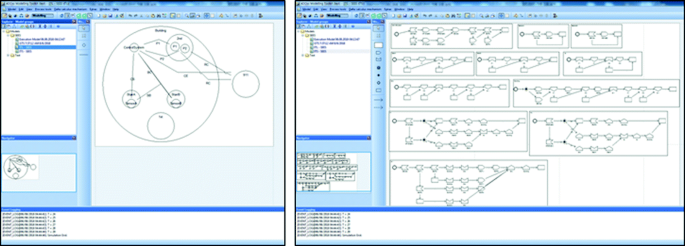
Specification tool of SAVE
-
(2)
Analyzer is a tool to generate the execution model from the specification in order to explore all the possible execution paths, as the left side of Fig. 10 shows, and to perform the simulation of each execution from the execution model in order to analyze probabilistic behaviors of the specified system.
Fig. 10. 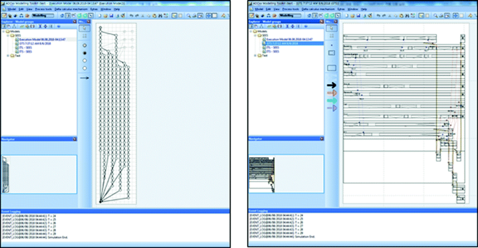
Analysis and verification tool of SAVE
-
(3)
Verifier is a tool to verify a set of system requirements on the geo-temporal space output generated from each, as the right side of Fig. 10 shows. It checks the behaviors of the system for safety and security requirements and shows their results on the output.


6 Conclusions and Future Research
This paper presented dTP-Calculus in order to model enterprise Smart IoT Systems, like Smart City, with uncertainty to safety and security of the systems. It showed that the algebra can be used to control the uncertainty with dynamic probability features on the unconditional nondeterministic choice operations, and that the algebra can provide good facilities to manage risks and capabilities with the systems. Further the paper presented the SAVE tool to demonstrate the feasibility of the approach with the calculus. It can be considered to be one of the innovative methods to handle the uncertainty for enterprise Smart IoT Systems.
The future research will include application of dTP-Calculus and SAVE to real enterprise industry examples to demonstrate their efficiency and effectiveness as method and tool.
References
Skouby, K.E., Lynggaard, P.: Smart home and smart city solutions enabled by 5G, IoT, AAI and CoT services. In: 2014 International Conference on Contemporary Computing and Informatics (IC3I), pp. 874–878. IEEE (2014)
Chin, J., Callaghan, V., Lam, I.: Understanding and personalising smart city services using machine learning, the Internet-of-Things and big data. In: 2017 IEEE 26th International Symposium on Industrial Electronics (ISIE), pp. 2050–2055. IEEE (2017)
Allam, Z., Dhunny, Z.A.: On big data, artificial intelligence and smart cities. Cities 89, 80–91 (2019)
Choe, Y., Lee, M.: Algebraic method to model secure IoT. Domain-Specific Conceptual Modeling, pp. 335–355. Springer, Cham (2016). https://doi.org/10.1007/978-3-319-39417-6_15
Meldal, S., Walicki, M.: Nondeterministic Operators in Algebraic Frameworks. Stanford University, Stanford (1995)
Feng, C., Hillston, J.: PALOMA: a process algebra for located Markovian agents. In: Norman, G., Sanders, W. (eds.) QEST 2014. LNCS, vol. 8657, pp. 265–280. Springer, Cham (2014). https://doi.org/10.1007/978-3-319-10696-0_22
Lee, I., Philippou, A., Sokolsky, O.: Resources in process algebra. J. Logic Algebraic Program. 72(1), 98–122 (2007)
Choe, Y., Lee, M.: Process model to predict nondeterministic behavior of IoT systems. In: Proceedings of the 2nd International Workshop on Practicing Open Enterprise Modelling within OMiLAB (PrOse) (2018)
Song, J., Choe, Y., Lee, M.: Application of probabilistic process model for smart factory systems. In: Douligeris, C., Karagiannis, D., Apostolou, D. (eds.) KSEM 2019. LNCS (LNAI), vol. 11776, pp. 25–36. Springer, Cham (2019). https://doi.org/10.1007/978-3-030-29563-9_3
Choe, Y., Lee, S., Lee, M.: dT-Calculus: a process algebra to model timed movements of processes. Int. J. Comput. 2, 53–62 (2017)
Choe, Y., Lee, S., Lee, M.: SAVE: an environment for visual specification and verification of IoT. In: 2016 IEEE 20th International Enterprise Distributed Object Computing Workshop (EDOCW), pp. 1–8. IEEE (2016)
Fill, H.G., Karagiannis, D.: On the conceptualisation of modeling methods using the ADOxx meta modeling platform. In: Proceedings of Enterprise Modeling and Information Systems Architectures (EMISAJ), vol. 8, no. 1, pp. 4–25 (2013)
Acknowledgment
This work was supported by Basic Science Research Programs through the National Research Foundation of Korea (NRF) funded by the Ministry of Education (2010-0023787), Space Core Technology Development Program through the National Research Foundation of Korea (NRF) funded by the Ministry of Science, ICT and Future Planning (NRF-2014M1A3A3A02034792), Basic Science Research Program through the National Research Foundation of Korea (NRF) funded by the Ministry of Education (NRF-2015R1D1A3A01019282), and Hyundai NGV, Korea, and Research Fund from Chonbuk National University (2018–2019).
Author information
Authors and Affiliations
Corresponding author
Editor information
Editors and Affiliations
Rights and permissions
Copyright information
© 2019 IFIP International Federation for Information Processing
About this paper

Cite this paper
Song, J., Lee, M. (2019). Process Algebra to Control Nondeterministic Behavior of Enterprise Smart IoT Systems with Probability. In: Gordijn, J., Guédria, W., Proper, H. (eds) The Practice of Enterprise Modeling. PoEM 2019. Lecture Notes in Business Information Processing, vol 369. Springer, Cham. https://doi.org/10.1007/978-3-030-35151-9_12
Download citation
DOI: https://doi.org/10.1007/978-3-030-35151-9_12
Published:
Publisher Name: Springer, Cham
Print ISBN: 978-3-030-35150-2
Online ISBN: 978-3-030-35151-9
eBook Packages: Computer ScienceComputer Science (R0)