
Abstract
In this chapter, we introduce our assumptions about semantic representations and build a semantic processor, that is, a basic parser able to incrementally construct such semantic representations. Our choice for a processing-friendly semantics framework is Discourse Representation Theory (DRT, Kamp 1981; Kamp and Reyle 1993).
You have full access to this open access chapter, Download chapter PDF
In this chapter, we introduce our assumptions about semantic representations and build a semantic processor, that is, a basic parser able to incrementally construct such semantic representations. Our choice for a processing-friendly semantics framework is Discourse Representation Theory (DRT, Kamp 1981; Kamp and Reyle 1993).
We build an ACT-R parser for Discourse Representation Structures (DRSs), and motivate the assumptions we make when building it by accounting for the fan experiment reported in Anderson (1974), as summarized and discussed in the more recent Anderson and Reder (1999).
The fan experiment investigates how basic propositional information of the kind encoded by atomic DRSsFootnote 1 is (stored and) retrieved from declarative memory. This is an essential component of real-time semantic interpretation in at least two respects:
-
i.
incrementally processing semantic representations involves composing/integrating semantic representations introduced by new sentences or new parts of a sentence with semantic representations of the previous discourse;
-
ii.
incremental interpretation also involves evaluating new semantic representations relative to our mental model of the world, and integrating their content into our world knowledge database stored in declarative memory.
The main reason for selecting DRT as our semantic framework is that atomic DRSs and the compositional construction principles used to build them provide meaning representations and elementary compositional operations that are well understood mathematically, widely used in formal semantics, and can simultaneously function as both meaning representations (logical forms, in linguistic parlance) and their content/world knowledge (models, in linguistic parlance).
Because of this double function, DRT and atomic DRSs can be thought of as mental models in the sense of Johnson-Laird (1983, 2004); Johnson-Laird et al. (1989), with several advantages. First, they provide a richer and better understood array of representations and operations. Second, they come with a comprehensive mathematical theory of their structure and interpretation (dynamic logic/dynamic semantics). Finally, they are well-known and used by linguists in the investigation of a wide variety of natural language semantic phenomena.Footnote 2
It is no accident that DRT is the most obvious choice for psycholinguistic models of natural language semantics. DRT has always had an explicit representational commitment, motivated by the goal of interfacing semantics and cognitive science more closely (Kamp 1981 already mentions this).
Importantly, DRT is a dynamic semantic framework, so it has a notion of DRS merge, that is, a merge of two (conjoined) representations into a larger representation of the same type. This DRS merge operation makes the construction, maintenance and incremental update of semantic representations more straightforward and, also, similar to the construction, maintenance and incremental update of syntactic representations.Footnote 3
DRT, however, is not the only possible choice as a way to add meaning representation to cognitive models of language comprehension. Less “representational” systems—whether dynamic, e.g., Dynamic Predicate Logic (DPL, Groenendijk and Stokhof 1991) or Compositional DRT (CDRT, Muskens 1996), or static, e.g., Montague’s Intensional Logic (IL, Montague 1973), variants of Gallin’s Ty3/Ty4/etc. (Gallin 1975) or partial/multivalued logics (Muskens 1995a)—are also possible, although less straightforwardly so, at least at a first glance.
The extent to which these alternative semantic frameworks are performance-friendly, that is, the extent to which they are fairly straightforwardly embeddable in a cognitive-architecture-based framework for mechanistic processing models, might provide a useful way to distinguish between them, and a plausible new metric for semantic theory evaluation. What we have in mind here is nothing new: Sag (1992) and Sag and Wasow (2011) argue persuasively that linguistic frameworks should be evaluated with respect to their performance-friendliness. The discussion there understandably focuses on syntactic frameworks, but it is easily transferable to semantics.
Our hope is that, once a set of ‘performance-friendly’ semantic frameworks are identified, and the ways of embedding them into explicit processing models for semantics are explored and motivated, the predictions of the resulting competence-performance models will enable us to empirically distinguish between these semantic frameworks.
The structure of this chapter is as follows. In the following Sect. 8.1, we introduce the fan-effect phenomenon and the original experiment reported in Anderson (1974) that established its existence. The fan effect provides a window into the way propositional facts—basically, atomic DRSs—are organized in declarative memory.
Section 8.2 discusses how DRSs can be encoded in ACT-R chunks, and makes explicit how the fan effect can be interpreted as reflecting DRS organization in declarative memory.
Sections 8.3 and 8.4 model the fan experiment by parsing the experimental items (simple English sentences with two indefinites) into DRSs, storing them in memory, and fitting the resulting model to the retrieval latencies observed in the experiment.
Parsing natural language sentences into DRSs is fully modeled: Sect. 8.3 explicitly models how experimental participants comprehend these sentences by means of a fully specified incremental parser/interpreter for both syntactic and semantic representations. This eager left-corner parser incrementally constructs the syntactic representations for the experimental sentences (phrase-structure grammar trees of the kind we already discussed in Chap. 4), and in parallel, it incrementally constructs the corresponding semantic representations, that is, DRSs.
Modeling the fan experiment in Anderson (1974) by means of this incremental syntax/semantics parser will enable us to achieve two goals. First, we shed light on essential declarative memory structures that subserve the process of natural language interpretation. Second, we introduce and discuss basic modeling decisions we need to make when integrating the ACT-R cognitive architecture and the DRT semantic framework.
Section 8.4 shows that the incremental syntax/semantics parser is able to fit the fan-effect data well, and Sect. 8.5 summarizes the main points of this chapter.
8.1 The Fan Effect and the Retrieval of DRSs from Declarative Memory
The fan effect
refers to the phenomenon that, as participants study more facts about a particular concept, their time to retrieve a particular fact about that concept increases. Fan effects have been found in the retrieval of real-world knowledge [...], face recognition [...] [etc.] The fan effect is generally conceived of as having strong implications for how retrieval processes interact with memory representations. It has been used to study the representation of semantic information [...] and of prior knowledge [...]. (Anderson and Reder 1999,186).
The original experiment in Anderson (1974) demonstrated the fan effect in recognition memory. Participants studied 26 facts about people being in various locations, 10 of which are exemplified in (1) below.

In the training part of the experiment, participants committed 26 items of this kind to memory. In the test part of the experiment, participants were presented with a series of sentences, some of which they had studied in the training part and some of which were novel. They had to recognize the sentences they had studied, i.e., the targets, and had to reject the foils, which were novel combinations of the same people and locations.
We selected the 10 items in (1) because, together, they form a minimal network of facts that instantiates the 9 experimental conditions in Anderson (1974). These conditions have to do with how many studied facts are connected to each type of person and location. To see this explicitly, we can represent the set of 10 facts in (1) as a network in which each fact is connected by an edge to the type/concept of person and location it is about, as shown in (2) below. Person concepts are listed on the left, and location concepts are listed on the right.

The network representation in (2) shows how different person and location concepts fan into 1, 2 or 3 sentences/facts. The table in (3) below shows how 9 of the 10 items exemplify the 9 conditions of the Anderson (1974) fan experiment (the 10th item is needed in our fact database to be able to instantiate all 9 conditions).

The table in (3) shows that the term ‘fan’ refers to the number of facts, that is, sentences, associated with each common concept, that is, noun. The mean reaction times (RTs, measured in s) for target recognition and foil rejection in the Anderson (1974) experiment are provided in the tables below (reproduced from Anderson and Reder 1999, p. 187, Table 2).

Several generalizations become apparent upon examining this data.

The ACT-R account of these generalizations, together with the quantitative fit to the data in (4) and (5), is provided in Andreson and Reder (1999, pp. 188–189). This account crucially relies on the spreading activation component of the ACT-R equation for activation of chunks in memory that we introduced in Chap. 6. Recall that the activation \(A_{i}\) of a fact/sentence i in memory is:

Base activation \(B_{i}\) is determined by the history of usage of fact i (how many times i was retrieved and how long ago), while the spreading activation component \(\sum \nolimits _{j}W_{j}S_{ji}\) boosts the activation of fact i based on the concepts j that fact i is associated with. Specifically, for each concept j, \(W_{j}\) is the extra activation flowing from concept j, and \(S_{ji}\) is the strength of the connection between concept j and fact i that modulates how much of the extra activation \(W_{j}\) actually ends up flowing to fact i.
The account of the fan effect observed in Anderson (1974) crucially relies on the strengths of association \(S_{ji}\) between concepts j and facts i. These strengths are modeled as shown below:

S is a constant (baseline strength) to be estimated for specific experiments, while P(i|j) is an estimate of the probability of needing fact i from declarative memory when concept j is present in the cognitive context, e.g., in the goal or imaginal buffers. That is, P(i|j) is an estimate of how predictive concept j is of fact i.
In an experimental setup in which all facts are studied and tested with equal frequency, it is reasonable to assume that the predictive probability P(i|j) is simply \(\frac{1}{\text{ fan }_{j}}\), where \(\text{ fan }_{j}\) is the fan of concept j. If a concept has a fan of 1, e.g., lawyer in (2) above, then the probability of the associated fact (1a) is 1. However, if a concept has a fan of 3, like hippie, all three facts associated with this concept, namely (1h), (1i) and (1j), are equiprobable, with a probability of \(\frac{1}{3}\).
Thus, for the experiment in Anderson (1974), the strength-of-association equation can be simplified to:

The equation in (9) implies that strength of association, and thereby fact activation, will decrease as a logarithmic function of concept fan. Strength/activation of a fact decreases with concept fan because the probability of a fact given a concept decreases with the fan of that concept. For more discussion of strength of association, source activation etc., see Sect. 6.3.
The last piece of the ACT-R model is the function that outputs retrieval latencies given fact activations. This is provided in (10) below, which should be familiar from Chaps. 6 and 7 (the latency exponent is omitted, i.e., set to its default value 1).

The only addition is the intercept I, which captures all cognitive activities other than fact retrieval, e.g., encoding the test sentence, generating the response etc. Recall that we used a similar intercept in Chap. 7 when we proposed the first two models of lexical decision—see Sects. 7.2 and 7.3
All of these model components will be made explicit in Sects. 8.3 and 8.4 below, where we provide the first end-to-end ACT-R model of the fan effect in the literature. No such models have been available because incremental semantic interpretation was never explicitly modeled in ACT-R before.
We can further simplify our mathematical model specification by putting together Eqs. (7), (9) and (10) as follows:

We can further assume that \(\sum \nolimits _{j}W_{j}\) is fixed and set to 1. This is motivated by the capacity limitations in retrieval discussed in Anderson et al. (1996). Finally, if we assume that the source activations \(W_{j}\) of all concepts j are equal, we can set them all to a constant W. The final form of the ACT-R model for fan-dependent retrieval latencies is therefore:

The latency equation in (12) shows how the ACT-R model captures the fan effect, i.e., the generalization in (6a) that recognition latency increases with fan. To see this more clearly, let’s apply this equation to the facts in the Anderson (1974) experiment. These facts are connected to 3 concepts (a person, a location, and the predicate in), so the source activation W is \(\frac{1}{3}\). The resulting latency equation is provided in (13).

The predicate in is connected to all the sentences/facts, so it will have a constant fan and it will contribute a constant amount of activation (hence latency) across all conditions in the experiment. But the person and location fan values \(\text{ fan }_{\textit{person}}\) and \(\text{ fan }_{\textit{location}}\) are manipulated in the experiment, and the equation in (13) correctly predicts that, as they increase, the corresponding latency T increases.
The equation in (13) also provides an account of the min effect (generalization (6b) above). The reason is that the product of a set of numbers with a constant sum, specifically the product \(\text{ fan }_{\textit{person}}\cdot \text{ fan }_{\textit{location}}\), is maximal when the numbers are equal, e.g., \(2\times 2 > 3\times 1\).
To understand how the ACT-R model captures the generalization in (6c), that is, the fact that foils are retrieved almost as quickly as target sentences, we need to specify the process of foil recognition. The main idea is that foil recognition does not involve an exhaustive search. Instead:

For simplicity, we can assume that participants retrieve the mismatching fact half the time with a person cue, and half the time with a location cue. Either way, mismatching facts have one less source of spreading activation coming from the foil sentence (which is encoded in the goal or imaginal buffer) than matching facts. Their total activation will therefore be lower, so the time to retrieve foils will be slightly higher than the time to retrieve targets.
By the same token, the correct fact will almost always be retrieved for target sentences because this fact will have more sources of spreading activation coming from the target sentence—hence a higher total activation—than any other incorrect fact in memory.
To be more specific, the activation of the correct fact given a target sentence is shown in (15) below. Recall that all source activations \(W_{\textit{person}}\), \(W_{\textit{location}}\) and \(W_{\textit{in}}\) are assumed to be \(\frac{1}{3}\).

All three terms \(\frac{S - \log (\text{ fan }_{\textit{person}})}{3}\), \(\frac{S - \log (\text{ fan }_{\textit{location}})}{3}\) and \(\frac{S - \log (\text{ fan }_{\textit{in}})}{3}\) are positive, so they each add an extra activation boost, hence an extra decrease in latency of retrieval.
In contrast, activation of foils has only 2 spreading activation terms. Either the location term is missing, as in (16a) below, where fact retrieval for the foil sentence is person-based, or the person term is missing, as in (16b), where fact retrieval for the foil sentence is location-based. Less spreading activation means lower total activation, which leads to slightly increased latency of retrieval.

This ACT-R model is sufficiently flexible to account for a range of effects beyond the original fan experiment in Anderson (1974). Different values for sources of activation \(W_{j}\) can account for differential fan effects associated with different types of concepts (inanimate objects versus persons, for example).
Similarly, different values for strengths of activation \(S_{ji}\) that depend on the frequency of presentation of fact-concept associations, which affect probabilities P(i|j), can account for retrieval interference effects that go beyond simple fan effects. For more discussion, see Anderson and Reder (1999).
However, for the remainder of this chapter, we will focus exclusively on the original fan experiment in Anderson (1974), and specifically on modeling retrieval latencies for the target sentences in (4). The next section reformulates the fan effect in terms of the way meaning representations (DRSs) that are associated with target sentences are organized in declarative memory.
8.2 The Fan Effect Reflects the Way Meaning Representations (DRSs) Are Organized in Declarative Memory
We can reformulate the notion of fan in Anderson ’s experiment, as well as the network of facts and concepts in (2) above, as a relation between the main DRS contributed by a sentence and the sub-DRSs contributed by its three parts: the person indefinite, the location indefinite, and the relational predicate in.
Consider the 1–1 fan (that is, 1 person–1 location fan) example in (1a), repeated in (17) below. The DRSs (meaning representations) of the three major components of the sentence, that is, the indefinites a lawyer and a cave, and the binary predicate it, are composed/combined together to form the DRS/meaning representation for the full sentence.
The exact nature of the three meaning components and the composition method vary from framework to framework. For example, the method of composition in Kamp and Reyle (1993) is a set of construction principles operating over hybrid representations combining DRSs and syntactic trees. The method of composition in Brasoveanu (2007, Chap. 3), building on much previous work (Groenendijk and Stokhof 1990; Chierchia 1995; Muskens 1995b, 1996 among others) is classical Montagovian function application/\(\beta \)-reduction operating over DRS-like representations, which are just abbreviations of terms in a many-sorted version of classical simply-typed lambda calculus (Gallin 1975). Finally, the method of composition in Brasoveanu and Dotlačil (2015b) (building on Vermeulen 1994 and Visser 2002) is dynamic conjunction over DRSs interpreted as updates of richly structured interpretation contexts that record information state histories.
However, we do not need to fully specify a semantic framework for natural language meaning representation and composition to reformulate the fan experiment in formal semantics/DRT terms. It is sufficient to acknowledge that the main DRS contributed by a sentence like (17) is formed out of three sub-DRSs, contributed by the two indefinites a lawyer and a cave, and the preposition in.
This partitioning into three sub-DRSs matches the rough compositional skeleton generally assumed in the formal semantics literature for this type of sentences, as well as the real-time incremental comprehension process the ACT-R architecture imposes on us.
Recall that, because of the seriality imposed in ACT-R by one production firing at a time, and by the imaginal buffer being able to hold only one chunk at a time, we never have a full view of the syntactic tree representation.
Similarly, we will never have a full view of the DRS semantic representation. This representation will be assembled one sub-DRS at a time, resulting in the main DRS in (18). But this ‘deep’, i.e., hierarchical, representation of the main DRS with the sub-DRSs actually encoded as values of its slots is only implicitly available in declarative memory, just like the full syntactic tree of the sentence in (17) is only implicitly available in declarative memory.

If we merge (i.e., dynamically conjoin and ‘reduce’) the three sub-DRSs into one DRS, we obtain the DRS in (19) below, which is precisely the semantic representation assigned to sentence (17) in DRT. It can be shown that this merged DRS is truth-conditionally equivalent to the classical first-order logic formula in (20),Footnote 4 which is the basic semantic representation that pretty much all static (neo-)Montagovian semantic frameworks derive for sentence (17).

Chunks like the one exemplified in (18) lend themselves fairly straightforwardly to modeling the fan experiment in Anderson (1974). But before we show how to do that, let’s take a further step and encode the sub-DRSs as chunks, i.e., as attribute-value matrices. One way to do it is as shown in (21) below:
-
first, we replace the variables/discourse referents x and y with subscripted variables, e.g., \(\nu _{1}\) and \(\nu _{2}\); actually, while we’re at it, we can drop \(\nu \) altogether and simply retain the indices \(1,2,\dots \) as variables/discourse referentsFootnote 5;
-
for example, \(\text{ lawyer }(x)\), \(\text{ cave }(y)\) and \(\text{ in }(x, y)\) become \(\text{ lawyer }(1)\), \(\text{ cave }(2)\) and \(\text{ in }(1, 2)\);
-
-
second, we separate DRS conditions into distinct features for the predicate and for its arguments;
-
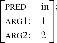
for example, the condition \(\text{ in }(1, 2)\) is replaced with the chunk/attribute value matrix
-
-
finally, sub-DRSs that introduce new discourse referents—that is, they contribute something like an implicit existential quantifier in addition to conditions—will have a new feature dref to indicate what new discourse referent they introduce;
-
for example, sub-drs\(_{1}\) in (21) introduces the new discourse referent 1, which is a lawyer, so 1 is both the value of the dref feature and the value of the arg1 feature (since it is the first, and only, argument of the ‘lawyer’ predicate).
-


The graph like representation of the chunk in (21) is provided in (22) below.

Since all the main DRSs for the items in (1) are going to be connected to the sub-drs\(_{3}\) contributed by the preposition in, we can omit that connection—and we will do that from now on.
With that omission in place, we can reproduce the network of facts and concepts in (2) more properly as a semantic network of DRSs in declarative memory. For space reasons, (23) below only provides the DRS network corresponding to the first four experimental items (1a) through (1d).

Structuring DRSs in memory as a network in which a main DRS contains, i.e., is connected to, sub-DRSs contributed by various sub-sentential expressions is reminiscent of the structured meanings approach to natural language semantics in Cresswell (1985).
We leave the exploration of further connections between the structure of meaning representations in declarative memory, semantic composition, incremental processing and various approaches to the formal semantics of propositional attitudes (structured meanings among others) for a future occasion.
8.3 Integrating ACT-R and DRT: An Eager Left-Corner Syntax/Semantics Parser
With these semantic assumptions in place, we are ready to specify our model for the Anderson (1974) fan experiment. The model we introduce in this section is the first model of a fan experiment to explicitly incorporate syntactic and semantic parsing.
In fact, this is the first end-to-end model of the testing phase of Anderson (1974) experiment, explicitly incorporating (i) a visual component (eye-movement while reading), (ii) a motor component (accept or reject whether the test sentence was studied in the training phase), and (iii) a syntax/semantics incremental interpreter for the test sentence as it is being read.
For simplicity, we focus exclusively on modeling target sentences, and the observed mean target latencies in (4) above. But the model will be designed with foils in mind too, and could be equally applied to model the mean foil latencies in (5) above.
The core component of our cognitive model for a participant in the Anderson (1974) fan experiment is an eager left-corner parser that parses syntactic trees and DRSs simultaneously and in parallel. As a new word is incrementally read in the usual left-to-right order for English:
-
the model eagerly and predictively builds as much of the syntactic and semantic representation as it can (before deciding to move the eyes to the next word);
-
this process of syntactic and semantic representation building is the process of comprehending the new word and integrating it into the currently available partial syntactic and semantic structure;
-
these cognitive actions of comprehension and integration result in a new partial syntactic and semantic structure;
-
in turn, this syntax/semantics structure provides the context relative to which the next word is interpreted, and which will be updated as this next word is comprehended and integrated.
The overall dynamics of parsing is thus very similar to dynamic semantics: a sequence of parsing actions or a sequence of dynamic semantics updates charts a path through the space of information states. Each info state provides both (i) the context relative to which a semantic update is interpreted and, at the same time, (ii) the context that is changed as a result of executing that update.
Information states are simpler for dynamic semantics: they are basically variable assignments or similar structures. For our ACT-R incremental parser, information states are complex entities consisting of the partial syntactic and DRS structure built up to that point, as well as the state of the buffers and modules of the ACT-R mind at that point in the comprehension process.
Our syntax/semantics parser builds semantic representations and syntactic structures simultaneously, but the two types of representations are independently encoded and relatively loosely connected. In particular, we will postulate a separate imaginal-like buffer, which we will label discourse_context, where DRSs are incrementally built. We will continue to store partial syntactic representations in the imaginal buffer.
The decision to build syntax/semantics representations simultaneously, but in separate buffers is in the spirit of the ACT-R architecture. We avoid integrating two complex representations directly in a single ‘super-chunk’, keeping chunk size relatively small and also keeping the chunks themselves relatively flat. By ‘flat’ chunks, we mean chunks without many levels of embedding, that is, without many features that have other chunks as values, whose features in their turn have other chunks as values etc.
These ‘deep’ hierarchical representations are ubiquitous in generative syntax and semantics, but they are not compatible with the view of (high-level) cognitive processes embodied by the ACT-R cognitive architecture, at least not immediately. Thus, it is important to note that the independently motivated ACT-R cognitive architecture places non-trivial constraints on the form of our linguistic performance models, and indirectly on our competence-level models.
We had to make many implementation decisions when we divided the syntax and semantics labor across buffers and productions, and some of these decisions could have been made differently. However, the resulting model is (we hope) pedagogically accessible, and is in keeping with most of the received wisdom about the properties of the human processor in the psycholinguistic literature (Marslen-Wilson 1973, 1975; Frazier and Fodor 1978; Gibson 1991, 1998; Tanenhaus et al. 1995; Steedman 2001; Hale 2011 among many others). While this received wisdom focuses mainly on the syntactic aspects of real-time language comprehension, the simplest way to extend it to semantics is to assume that it applies in basically the same form and to the same extent (if possible).
Specifically, the human processor, and our model of it, is incremental since syntactic parsing and semantic interpretation do not lag significantly behind the perception of individual words. It is also predictive since the processor forms explicit syntactic and semantic representations of words and phrases that have not yet been heard. Finally, it satisfies the competence hypothesis because the incremental interpretation process requires the recovery of a grammar-based structural description on the syntax side, and of a meaning representation (DRS) on the semantic side.
Furthermore, the syntax and semantics parsing process we implement formalizes fairly directly the general view of sentence comprehension summarized in Gibson (1998, p. 11):
Sentence comprehension involves integrating new input words into the currently existing syntactic and discourse structure(s). Each integration has a syntactic component, responsible for attaching structures together, such as matching a syntactic category prediction or linking together elements in a dependency chain. Each integration also has a semantic and discourse component which assigns thematic roles and adds material to the discourse structure. (Gibson 1998, p. 11)
Let us now turn to an example and show how our model incrementally interprets the sentence in (17/1a) above, namely:
Assume that the first word, i.e., the indefinite article a, has already been read and recognized as a determiner. At that point, the "project: NP ==> Det N" rule in (24) below is selected and fired.

First, note that:
-
the lexical entry for the determiner a is assumed to be available in the retrieval buffer (lines 10–12 in (24));
-
our current top goal is to parse an S (line 5);
-
a fresh discourse referent index, a.k.a. dref_peg, is available in the goal buffer (line 9).
The value of the dref_peg feature is assigned to an ACT-R variable =peg that will be used in the cognitive actions triggered by this rule. The index =peg is fresh in the sense that no discourse referent with that index has been introduced up to this point. Thus, that index has never been part of the semantic representation up until now: it was never the argument of a predicate, it couldn’t have served as the antecedent for a pronoun etc. The term ‘peg’ and its specific usage here originates in Vermeulen (1995).
Given these preconditions, the rule in (24) simultaneously builds:
-
a syntactic representation in the imaginal buffer (lines 21–26), and
-
a semantic representation in the discourse_context buffer (lines 27–30).
In the imaginal buffer, we build the unary branching node NP dominating the Det node, which in turn dominates the terminal a.
In the discourse_context buffer, we start a new DRS that will be further specified by the upcoming N (lawyer). This DRS introduces a new discourse referent with the index =peg, and also requires this discourse referent to be the first argument (arg1) of the still-unspecified predicate contributed by the upcoming N—and also the first argument of the subsequent VP, as we will soon see.
In the more familiar format, the DRS contributed by rule (24) to the discourse_context buffer is provided in (25) below. Note that the value of the =peg index is specified as 1 since this is the first discourse referent introduced in the sentence.

The semantic part of the production rule in (24)—and the way it sets up the interpretation context for the upcoming N and VP—is very similar to the meaning assigned to the singular indefinite determiner a in dynamic semantic frameworks. For example, the indefinite a is associated with the following kind of meaning representation in Compositional DRTFootnote 6:

The subscripted type \(\mathbf {et}\) in (26) ensures that \(P'\) and P are (dynamic) properties. These properties will be contributed by the upcoming N lawyer and the subsequent VP is in a cave. The new discourse referent 1 introduced by the indefinite is superscripted on the indefinite a itself, and it is marked as newly introduced in the semantic representation by square brackets [1]. The semicolon ‘; ’ is dynamic conjunction (familiar from imperative programming languages like C).
Technically, the meaning representation in (26) is a function-denoting term in (classical, static) many-sorted simply-typed higher-order logic. However, it can be paraphrased as a sequence of update instructions. Specifically, the indefinite determiner a\(^{1}\) ‘says’ that:
-
once two properties \(P'\) and P are given to me in this specific order (\(\lambda P'_{\mathbf {et}}.\lambda P_{\mathbf {et}}.\)),
-
I will introduce a new discourse referent/‘variable’ ([1]),
-
then (;),
-
I will check that the discourse referent satisfies the first property (\(P'(1)\)),
-
and then (;),
-
I will check that the discourse referent satisfies the second property (P(1)).
We will see that our processing model follows this semantic ‘recipe’ fairly closely, but it distributes it across:
-
i.
several distinct productions in procedural memory,
-
ii.
several distinct chunks sequentially updated and stored in the discourse_context buffer, and
-
iii.
specific patterns of information flow, that is, feature-value flow, between the g (goal), imaginal and discourse_context buffers.
In addition to adding chunks to the imaginal and discourse_context buffers, the production rule in (24) above also specifies a new task in the goal buffer, which is to move_peg (line 16 in (24)). This will trigger a rule that advances the ‘fresh discourse referent’ index to the next number. In our case, it will advance it to 2. This way, we ensure that we have a fresh discourse referent available for any future expression, e.g., another indefinite, that might introduce one.
We also have a new stack of expected syntactic categories in the goal buffer (lines 17–19 in (24)). We first expect an N, at which point we will be able to complete the subject NP. Once that is completed, we can return to our overarching goal of parsing an S.
We will not discuss the family of move_peg rules. The full code is linked to in the appendix to this chapter—see Sect. 8.6.2. Instead, we will simply assume that the discourse reference peg has been advanced and discuss the "project and complete: N" rule in (27) below. This is the production rule that is triggered after the word lawyer is read and its lexical entry is retrieved from declarative memory.

The "project and complete: N" rule requires the lexical entry for an N (lawyer, in our case) to be in the retrieval buffer (lines 11–14 in (27)). It also requires the top of the goal stack, that is, the most immediate syntactic expectation, to be N (line 5). Finally, the rule checks that there is a DRS in the discourse_context buffer (lines 15–16). This is the DRS contributed by the preceding determiner a, and which will be further updated by the noun lawyer.
Once all these preconditions are satisfied, the "project and complete: N" rule triggers a several actions that update the current parse state, i.e., the current syntactic and semantic representations.
First, a new part of the tree is added to the imaginal buffer (lines 24–30): this is the binary branching node NP with two daughters, a Det on the left branch and an N on the right.
Second, the DRS in the discourse_context buffer that was introduced by the determiner a is updated with a specification of the pred feature (lines 31–33). Specifically, the predicate =p on line 33 is the one contributed by the lexical entry of the word lawyer, which is currently available in the retrieval buffer (see line 14).
After the "project and complete: N" rule in (27) above fires, the DRS in the discourse_context buffer becomes:

Note that at this point, the discourse_context buffer holds sub-drs\(_{1}\) of the Main-drs in (18/21).
With the subject NP a lawyer now completely parsed, both syntactically and semantically, we have the full left corner of the ‘S \(\rightarrow \) NP VP’ grammar rule, so we can trigger it. The corresponding production rule "project and complete: S ==> NP VP" is provided in (29) below.

This production rule eagerly discharges the expectations for an NP and an S from the goal stack (lines 6–7 in (29)) and replaces them both with a VP expectation (line 16). At the same time, a new part of the syntactic tree is built in the imaginal buffer, namely the top node S and its two daughters NP and VP (lines 21–25).
Finally, one important semantic operation happens in this rule, namely the transfer of the discourse referent =d from the discourse_context buffer (line 12) to the top of the argument stack arg_stack in the goal buffer (line 20). This operation effectively takes the discourse referent 1 introduced by the subject NP a lawyer and makes it the first argument of the VP we are about to parse. That is, this is how the cognitive process implements the final P(1) semantic operation/update in formula (26) above.
We can now proceed to parsing the copula is, which we take to be semantically vacuous for simplicity. As the rule in (30) shows, the copula (once read and lexically retrieved) simply introduces a new part of the syntactic tree: the VP node with a Vcop (copular verb) left daughter and a PP right daughter.

We can now move on to the preposition in. Once this preposition is read and lexically retrieved, the rule "project and complete: PP ==> P NP" in (31) below is triggered.

The preconditions of the rule in (31) are the following: (i) the top of the goal stack is a PP (line 6), (ii) the argument stack stores the discourse referent =a contributed by the subject NP (line 8), and (iii) the retrieval buffer contains the lexical entry of the preposition, specifically the predicate =p contributed by it (line 13). If these preconditions are satisfied, the following cognitive actions are triggered:
-
replace the PP at top of the goal stack with an NP (line 17); this is the NP that we expect the preposition to have as its complement;
-
build a new part of the syntactic tree in the imaginal buffer, with PP as the mother node and daughters P and NP (lines 18–24);
-
add a new DRS to the discourse_context buffer, the predicate of which is the binary relation =p contributed by the preposition, and the first argument of which is the subject discourse referent =a (lines 25–28);
-
finally, flush the retrieval buffer (line 29).
While the syntactic components of the PP rule in (31) are specific to prepositions, the semantic part is more general: this is how binary relations (transitive verbs like devour, relational nous like friend or aunt etc.) are all supposed to work. They contribute their predicate =p to a new DRS and they specify the first argument of their binary relation to be the discourse referent =a contributed by the subject NP, as shown in (32) below.
Note that the DRS has an empty universe because no new discourse referents are introduced. Also, the second argument of the IN binary relation is still unspecified (symbolized by ‘_’) because the location NP a cave, which will provide that argument, has not yet been read and interpreted.

We can now move on to the location NP a cave. Once the indefinite determiner a is read and lexically retrieved, the "project and complete: NP ==> Det N" rule in (33) below is triggered. Note that this rule is different from the "project: NP ==> Det N" in (24) above. The earlier "project NP" rule is triggered for subjects, that is, for positions where an NP is not already expected, i.e., it is not already present at the top of the goal stack.
The "project and complete NP" rule is triggered for objects of prepositions, transitive verbs etc. since these are expected NPs. By expected NPs, we mean that an NP is already present at the top of the goal stack when the determiner is read, as shown on line 6 in (33) below.

The syntactic contribution of the rule in (33) is simply adding an NP node with a Det daughter to the imaginal buffer (lines 20–25). The semantic contribution is two-fold.
First, the DRS introduced by the preposition in is further specified by introducing a new discourse referent and setting the second argument slot of the in predicate to this newly introduced discourse referent (lines 26–29). The resulting DRS, provided in (34) below, is the same as sub-drs\(_{3}\) in (18/21) above, with the modification that the new discourse referent 2 is introduced in this sub-DRS rather than in sub-drs\(_{2}\). We return to this issue below.
At this point, we have completely assembled (a version of) sub-drs\(_{3}\) in the discourse_context buffer.

The second semantic contribution made by rule (33) above is the addition of a new DRS to the discourse_context buffer (lines 30–32) that will be our location DRS, i.e., sub-drs\(_{2}\) in (18/21). We simply specify that the newly introduced discourse referent 2 is the first argument of a yet unspecified predicate, to be specified by the upcoming noun cave. This DRS is provided in (35) below.

Unlike sub-drs\(_{2}\) in (18/21), the DRS in (35) has an empty universe, since we introduced discourse referent 2 in the DRS previously stored in the discourse_context buffer. For the simple example at hand (A lawyer is in a cave), the decision to introduce discourse referent 2 in sub-drs\(_{3}\) (34) rather than in sub-drs\(_{2}\) (35) is inconsequential: the ultimate semantic representation, i.e., merged DRS, will have the same form as in (19) above.
We decided to go with this way of encoding the introduction of object NP discourse referents rather than with the more standard semantic representation in (18/21) just to show that it is possible. Also, from a processing perspective, it is simpler and more natural to introduce a discourse referent at the earliest point in the left-to-right incremental interpretation process where the referent appears as the argument of a predicate.
This decision, however, unlike the standard formal semantics decision in (18/21), makes incorrect predictions with respect to the quantifier scope potential of the location NP. This is truth-conditionally inconsequential in our example because the subject NP is also an existential. But if the subject NP had been a universal quantifier, e.g., every lawyer, we would incorrectly predict that the location NP a cave can have only narrow scope relative to that quantifier. This is because its scope is tied to the point of discourse referent introduction, namely the predicate in. While this narrow-scope prediction is correct for so-called ‘semantically incorporated’ NPs, e.g., bare plurals (see Carlson 1977, 1980; Farkas and de Swart 2003 among others for more discussion), it is not generally correct for bona fide indefinite NPs, which are scopally unrestricted (see, for example, Brasoveanu and Farkas 2011 for a relatively recent discussion).
The semantic representation that makes correct scopal predictions is easy to obtain in this case: the discourse referent introduction on line 28 of (33) simply needs to be moved further down, e.g., immediately after line 31. In general, however, such a change might be non-trivial.
What we have here is an instance of a more general phenomenon: incremental processing order and semantic evaluation order do not always coincide (see Vermeulen 1994; Milward and Cooper 1994; Chater et al. 1995 for insightful discussions of this issue). We believe that the Bayes+ACT-R+DRT framework introduced in this book provides the right kind of formal infrastructure to systematically investigate this type of discrepancies between processing and semantic evaluation order. A detailed systematic investigation of such discrepancies will likely constrain in non-trivial ways both competence-level semantic theories and semantically-informed processing theories and models.
Once the final noun cave is read and lexically retrieved, a second application of the "project and complete: N" rule in (27) above is triggered. The semantic contribution of this rule is to further specify the DRS in (35) by adding the predicate. The resulting DRS is provided in (36) below, and is the final version of sub-drs\(_{2}\) produced by our syntax/semantics parser.

8.4 Semantic (Truth-Value) Evaluation as Memory Retrieval, and Fitting the Model to Data
At this point, our model has completely parsed the test sentence A lawyer is in a cave. With the DRS for this sentence in hand, we can move to establishing whether the sentence was studied in the training phase or not.
To put it differently, the training phase presented a set of facts, and now we have to evaluate whether the test sentence is true or not relative to those facts. That is, we view semantic (truth-value) evaluation as memory retrieval.Footnote 7
Thus, the bigger picture behind our DRT-based model of the fan effect is that the process of semantic interpretation proceeds in two stages, similar to the way interpretation proceeds in DRT.
In the initial stage, we construct the semantic representation/DRS/mental discourse model for the current sentence. In DRT, specifically in Kamp and Reyle (1993), this stage involves a step-by-step transformation of a complete syntactic representation of the sentence into a DRS by means of a series of construction-rule applications. In our processing model, this stage consists of applying an eager, left-corner, syntax-and-semantics parser to the current test sentence.
In the second stage, we evaluate the truth of this DRS/mental model by connecting it to the actual, ‘real-world’ model, which is our background database of facts stored in declarative memory. In DRT, the second stage involves constructing an embedding function (a partial variable assignment) that verifies the DRS relative to the model. In our processing model, truth/falsity evaluation involves retrieving—or failing to retrieve—a fact from declarative memory that has the same structure as the DRS we have just constructed.
Let us turn now to how exactly we model semantic evaluation as memory retrieval. First, we assume that all the facts studied in the training phase of the fan experiment are stored in declarative memory before we even start parsing the test sentence. All the relevant code is linked to in the appendix of this chapter (see Sect. 8.6.1). We will list here only the lawyer-cave fact, together with the type declarations for main DRSs and (sub)DRSs:

The three sub-DRSs are declared on lines 4–7 in (37) with the makechunk method, and are assigned to three Python3 variables (note: not ACT-R variables). We can then use these three Python3 variables as subparts/values inside the main DRS encoding the lawyer-cave fact (lines 8–9). Finally, we add the entire fact to declarative memory with the dm.add method (also lines 8–9).
The declarative memory module of our model is loaded with all the facts listed in (1) before the parsing process for a test sentence even starts. When the parse of a test sentence is completed, we have the location DRS, that is, subdrs\(_{2}\) in the discourse_context buffer. For the sentence we parsed in the previous section, that location DRS is provided in (36) above.
To set up the proper spreading-activation configuration for the fan-effect experiment, we have to have all three sub-DRSs that are produced during parsing in the goal buffer. Since only the location DRS is available, we have to recall the person DRS and the in DRS listed in (31) and (34) above so that we can add them to the goal buffer.
We start by recalling the in-relation DRS with the rule in (38) below. This rule is triggered as soon as the test sentence has been completely parsed: the task is still parsing (line 5), but the goal stack is empty (the top of the stack is None—line 6). For good measure, we also check that the last DRS that was constructed (the location DRS) is still in the discourse_context buffer (lines 7–8). Assuming these pre-conditions are satisfied, we place a retrieval request for a DRS—any DRS (lines 13–15). Because the in DRS is the one that was most recently added/harvested to declarative memory, it has the highest activation, and this is the DRS we will end up retrieving.

The retrieval request, however, doesn’t simply state that we should retrieve a chunk of type drs (line 14 in (38) above), but goes ahead and requires a non-empty arg1 feature (line 15). This extra-specification seems redundant, but it is in fact necessary: recall that the identity of a chunk (and of a chunk type) is given by its list of features, not by the name we give to the type. The type name listed as the value of the feature isa is simply a convenient abbreviation for us as modelers. Therefore, placing a retrieval request with a cue consisting only of isa drs is tantamount to placing a retrieval request for any chunk in declarative memory, whether it is of type drs, or main_drs, or indeed any of the other types we use (parsing_goal, parse_state and word—see the beginning of Sect. 8.6.1 for all chunk-type declarations). To make sure we actually place a retrieval request for a DRS, we need to list one of its distinguishing features, and we choose the arg1 feature here.
In addition to placing a retrieval request for the DRS with the highest activation, which is the in DRS, the rule in (38) also updates the task in the goal buffer to recall_person_subdrs. This sets the cognitive context up for the next recall rule, provided in (39) below. The preconditions of this rule include a full discourse_context buffer, where the location DRS is still stored (lines 9–10 in (39)), and a full retrieval buffer, which stores the successfully retrieved in DRS (lines 7–8).

Once these preconditions are satisfied, the rule will take the in DRS in the retrieval buffer and store it in the goal buffer under an expected3 feature (line 15). Encoding the in DRS as the value of the expected3 feature indicates that this DRS is expected to be subdrs\(_{3}\) of the verifying fact for the test sentence we just finished parsing.Footnote 8
Importantly, setting the in DRS as the value of a feature in the goal buffer ensures that there is spreading activation from this sub-DRS to all the main DRSs/facts in declarative memory that contain it. This is essential for appropriately modeling the fan effect.
More generally, at this point in the cognitive process, our goal is to add all three parsed sub-DRSs to the goal buffer (we still have to add the location and person sub-DRSs), so that we have spreading activation from each of them to main DRSs in declarative memory. Once we achieve this state for the goal buffer, we will be able to semantically evaluate the parsed test sentence. That is, we will place a retrieval request for a main DRS that can verify it.
In order to store all the sub-DRSs of the parsed test sentence in the goal buffer, we have to place one final retrieval request to recall the person DRS (lines 16–20 in (39)), which was the first semantic product of our process of parsing the test sentence. Crucially, this request is modulated by the constraint of not retrieving a DRS that was recently retrieved (lines 16–17 in (39)). This additional constraint is essential: had it not been present, the actual retrieval request for a DRS (any DRS) on lines 18–20 would end up retrieving the in DRS all over again. The reason for this is that the in DRS was the most activated to begin with, and its most recent retrieval triggered by the rule in (38) above boosted that activation even further.
The constraint to retrieve something that was not recently retrieved (lines 18–20 in (39)) is not ad hoc. This type of constraint is necessary in a wide variety of processes involving refractory periods after a cognitive action, and it is modeled in ACT-R (and pyactr) in terms of Pylyshyn ’s FINSTs (fingers of instantiation).
The original motivation for the FINST mechanism in early visual perception is summarized in Pylyshyn (2007):
When we first came across this problem [of object identity tracking that occurs automatically and generally unconsciously as we perceive a scene] [i.e., the need to keep track of things without a conceptual description using their properties] it seemed to us that what we needed is something like an elastic finger: a finger that could be placed on salient things in a scene so we could keep track of them as being the same token individuals while we constructed the representation, including when we moved the direction of gaze or the focus of attention. What came to mind is a comic strip I enjoyed when I was a young comic book enthusiast, called Plastic Man. It seemed to me that the superhero in this strip had what we needed to solve our identity-tracking or reidentification problem. Plastic Man would have been able to place a finger on each of the salient objects in the figure. Then no matter where he focused his attention he would have a way to refer to the individual parts of the diagram so long as he had one of his fingers on it. Even if we assume that he could not detect any information with his finger tips, Plastic Man would still be able to think ‘this finger’ and ‘that finger’ and thus he might be able to refer to individual things that his fingers were touching. This is where the playful notion of FINgers of INSTantiation came on the scene and the term FINST seems to have stuck. (Pylyshyn 2007, pp. 13–14)
ACT-R/pyactr uses the FINST mechanism in the visual module, and also generalizes it to other perception modules, including declarative memory, which, as Anderson (2004) puts it, is the perception module for the past.
Specifically, the declarative module maintains a record of the n most recent chunks that have been retrieved (\(n=4\) by default). These are the chunks indexed by a FINST. The FINST remains on them for a set amount of time (3 s by default), after which the FINST is removed and the chunk is no longer marked as recently retrieved.
Retrieval requests can specify whether the declarative memory search should be confined to chunks that are—or are not—indexed by a FINST. In rule (39), we require the DRS retrieval request on lines 18–20 to target only DRSs that have not been recently retrieved (lines 16–17), i.e., the retrieval request targets only non-FINSTed DRSs.
Let us summarize the state of the ACT-R mind, i.e., the cognitive context, immediately after the production rule in (39) fires:
-
the discourse_context buffer still contains the location DRS;
-
the expected3 feature in the goal buffer (for expected subdrs\(_{3}\)) has the in DRS as its value; this in DRS has just been retrieved from declarative memory;
-
finally, we have just placed a retrieval request for the person DRS, restricted to non-FINSTed DRSs to avoid retrieving the in DRS all over again.
Once this retrieval request is completed, we are ready to fire the rule in (40) below. We ensure that this rule fires only after the retrieval request is completed by means of the precondition on lines 8–9, which requires the retrieval buffer to be in a non-busy/free state.

When its preconditions are met, the rule in (40) finishes setting up the correct environment for spreading activation required by the fan experiment. This means that the three sub-DRSs that we constructed during the incremental interpretation of our test sentence have to be added to the goal buffer.
The previous rule already set the in DRS as the value of the expected3 feature of the goal buffer. We now set the person DRS, who has just been retrieved, as the value of the expected1 feature of the goal buffer (line 16 in (40)), and the location DRS, who has been in the discourse_context buffer since the end of the incremental parsing process, as the value of the expected2 feature (line 17 in (40)).
All three sub-DRSs in the goal buffer spread activation to declarative memory, giving an extra boost to the correct fact acquired during the training phase of the experiment.
We are now ready to semantically evaluate the truth/falsity of the test sentence. That is, we are ready to place a memory retrieval request for a main_drs/fact in declarative memory that makes the test sentence true.
Following the ACT-R account of the fan effect proposed in Anderson and Reder (1999), which we discussed in Sect. 8.1 above, we can place this memory retrieval request via the person sub-DRS, or via the location sub-DRS (see the discussion of foil identification in particular). On lines 18–20 of the rule in (40), we place the retrieval request with the person sub-DRS as the cue (the person sub-DRS is in the retrieval buffer).
Note the difference between the role that three sub-DRSs play as values that spread activation and the role that the person DRS plays as a retrieval cue/filter. Using the person DRS as a filter eliminates any main DRS that does not have the matching person DRS. In contrast, spreading activation only boosts the activation of the main DRSs in declarative memory that happen to store the same person, location and in relation, but it does not filter anything out. This means that recalling the main DRS by the person sub-DRS must result in retrieving one of those main DRSs that match the person sub-DRS, but it is possible that the recalled DRS will have a mismatching location sub-DRS, e.g., if spreading activation plays a very small role.
We can alternatively place the retrieval request with the location DRS as cue, as shown on lines 19–21 of the rule in (41) below. This rule is identical to the rule in (40) except that the retrieval cue is now the location DRS stored in the discourse_context buffer.

The rules in (40) and (41) are alternatives to each other, and either of them can be selected to fire. When running simulations of this model, we can simply leave it to pyactr to select if the retrieval of the main_drs should be in terms of the person sub-DRS (hence, rule (40)) or in terms of the location sub-DRS (hence, rule (41)). In the long run, each of these two rules will be selected about half the time, and the resulting RTs for targets and foils will be the average of person and location based retrieval (with a small amount of noise).
But if we want to eliminate this source of noise altogether, we can force the model to choose one rule in one simulation, and the other rule in a second simulation, and average the results. This is the option we pursue here. To achieve this, we make use of production-rule utilities, which induce a preference order over rules that is used when the preconditions of multiple rules are satisfied in a cognitive state. In that case, the rule with the highest utility is chosen.
To average over the recall-by-person and recall-by-location rules, we set the utility of recall-by-person rule in (40) to 0.5 (see line 21 in (40)), and we assign the recall-by-location rule in (41) to a Python3 variable recall_by_location (line 1 in (41)). With these two things in place, we can update the utility of the recall_by_location rule either to 0, which is less than the 0.5 utility of the recall-by-person rule, or to 1, which is more than 0.5. In the first case, the recall-by-person rule in (40) fires. In the second case, the recall-by-location rule in (41) fires.
In our Bayesian model, we can run two simulations with these two utilities for the recall-by-location rule, and take their mean. This is what the Bayesian estimation code linked to in Sect. 8.6.4 at the end of the chapter actually does. The relevant bit of code is provided in (42) below for ease of reference.Footnote 9

Once the retrieval request for the main_drs verifying the test sentence is completed, the rule in (43) below fires. This rule checks that the retrieved main_drs matches the DRS of the parsed test sentence with respect to the person and location DRSs stored in the goal buffer (lines 5–6 and 12–13). If this condition is met, the test sentence is declared true (it is part of the set of facts established in the training phase) and the ’J’ key is pressed (line 18–21). This concludes the simulation, so the goal buffer is flushed (line 17).

The model includes three other rules "mismatch in person found", "mismatch in location found" and "failed retrieval", provided in the code linked to at the end of the chapter in Sect. 8.6.2. These rules enable us to model foil retrieval and deal with cases in which a main_drs retrieval fails completely. But in this chapter, we focus exclusively on modeling target sentences, i.e., test sentences that were seen in the training phase, and for which the main_drs retrieval request succeeds.
The full model can be seen in action by running the script run_parser_fan.py, linked to in Sect. 8.6.3 at the end of the chapter. The model reads the sentence A lawyer is in a cave displayed on the virtual screen, incrementally interprets/parses it and checks that it is true relative to the database of facts/main DRSs in declarative memory.
The script estimate_parser_fan.py linked to in Sect. 8.6.4 embeds the ACT-R model into a Bayesian model and fits it to the experimental data from Anderson (1974). We do not discuss the code in detail since it should be fairly readable at this point: it is a variation on the Bayes+ACT-R models introduced in Chap. 7. Instead, we’ll highlight the main features of the Bayesian model.
First, we focus on estimating four subsymbolic parameters:
-
"buffer_spreading_activation" ("bsa" for short), which is the W parameter in Sect. 8.1 above;
-
"strength_of_association" ("soa" for short), which is the S parameter in Sect. 8.1 above;
-
"rule_firing" ("rf" for short), which is by default set to 50 ms;
-
"latency_factor" ("lf" for short).
Our discussion in Sect. 8.1 above shows that we need to estimate the "bsa", "soa" and "lf" parameters. We have also decided to estimate the "rf" parameter, instead of leaving it to its default value of 50 ms, because it is reasonable for it to be lower for the kind of detailed, complex language models we are constructing. In these models, multiple theoretically motivated rules are needed to fire rapidly in succession, and the total amount of time they can take is highly constrained by the empirical generalization that people take around 300 ms to read a word in an eye-tracking experiment, and they take roughly the same amount in a self-paced reading experiment.
We might be able to revert to the ACT-R default of 50 ms per rule firing if we take advantage of production compilation, which is a process by which multiple production rules and retrieval requests can be aggregated into a single rule. Production compilation is one of the effects of skill practice, and it is very likely that incremental interpretation of natural language, which is a highly practiced skill for adult humans, takes full advantage of it (see Chap. 4 in Anderson 2007 and, also, Taatgen and Anderson 2002 for more discussion of production compilation).
Production compilation is available in pyactr and we could make use of it in future developments of this model. However, production compilation will result in production rules that do not transparently reflect the formal syntax and semantics theories we assume here, making the connection between processing and formal linguistics more opaque.
It might very well be that more mature cognitive models of syntax and semantics will have to head in the direction of significant use of production compilation. However, we think that at this early point in the development of computationally explicit processing models for formal linguistics, it is more useful to see that established linguistic theories can be embedded in language processing ACT-R models in an easily recognizable fashion.
At the same time, we also want to show that the resulting processing models can fit experimental data well, and can provide theoretical insight into quantitatively-measured cognitive behavior.
To meet both of these desiderata, we need to depart from various default values for ACT-R subsymbolic parameters. In particular, for the semantic processing models in this chapter and the next one, we need to allow the "rf" parameter to vary and we need to estimate it. As we will soon see, the estimated value hovers around 10 ms, that is, it is significantly less than the ACT-R default. The need to lower ACT-R defaults when modeling natural language phenomena in a way that is faithful to established linguistic theories is a common thread throughout this book.
As shown in (44) below, the Bayesian model (i) sets up low information priors for these four parameters, (ii) runs the pyactr model to compute the likelihood of the experimental data in (4) above, and (iii) estimates the posterior distributions for these four parameters given the priors and the observed data. Links to the full code are provided in Sect. 8.6.4 at the end of the chapter.

The posterior estimates for the four parameters are provided in Fig. 8.1. The most notable one is the rule firing parameter, whose mean value is 11 ms rather than 50 ms. We will see that a similar value is necessary when we model cataphoric pronouns and presuppositions in the next chapter.

Fan model estimates

Fan model: observed versus predicted RTs
Note that the Rhat values for this model are below 1.1:

As the plot of the posterior predictions of the model in Fig. 8.2 shows, the model is able to fit the data fairly well. There are slight discrepancies between the predictions of the model and the actual observations, which are due to variance in the data that our fan model ignores from the start. For instance, when we inspect the table in 4, we see that the mean reaction time to recognize targets with a fan of 3 for person and a fan of 1 for location was 1.22 s, while the mean reaction time to recognize targets with a fan of 3 for location and a fan of 1 for person was 1.15 s. This difference of 70 ms cannot be captured by our model, which treats the two cases as identical.
We see that the model captures a large portion of the variance in data, but there is room for improvement. The model can in principle be enhanced in various ways if contrasts like the one we just mentioned turn out to be genuine and robust rather than largely noise, which is our current simplifying assumption.
8.5 Model Discussion and Summary
In this chapter, we modeled the fan experiment in Anderson (1974), bringing together the ACT-R account in Anderson and Reder (1999) and formal semantics theories of natural language meaning and interpretation. The resulting incremental interpreter is the first one to integrate in a computationally explicit way (i) dynamic semantics in its DRT incarnation and (ii) mechanistic processing models formulated within a cognitive architecture.
In developing this cognitive model, we argued that the fan effect provides fundamental insights into the memory structures and cognitive processes that underlie semantic evaluation. By semantic evaluation, we mean the process of determining whether something is true or false relative to a database of known facts/DRSs, i.e., relative to a model in the sense of model-theoretic semantics.
Future directions for this line of research include investigating whether a partial match of known facts is considered good enough for language users in comprehension. This could provide an integrated account of a variety of interpretation-related phenomena: (i) Moses illusions (see Budiu and Anderson 2004 for a relatively recent discussion), (ii) the way we interpret sentences with plural definites like The boys jumped in the pool, where the sentence it true without every single boy necessarily jumping in the poolFootnote 10, and (iii) ‘partial presupposition resolution’ cases, where part of the presupposition is resolved and part of it is accommodated (see Kamp 2001a for an argument that this kind of mixture of resolution and accommodation seems to be the rule rather than the exception).
Spreading activation in general can be used for predictive parsing: words (more generally, linguistic information) in the previous context can predictively activate certain other words, i.e., induce expectations for other chunks of linguistic information.
Another direction for future research is reexamining the decisions we made when developing our incremental DRT parser that were not based on cognitive plausibility, but instead were made for pedagogical reasons—in an effort to ensure that the contributions made by semantic theories were still recognizable in the final syntax/semantics parser. These decisions led to unrealistic posterior estimates, e.g., 11 ms for rule firing, which is not a fully satisfactory outcome.
In addition, we oversimplified the model in various ways, again for pedagogical purposes. For example, we initiated the semantic evaluation process (the search for a matching fact in declarative memory) only when the sentence was fully parsed syntactically and semantically. This is unrealistic: parsing, disambiguation and semantic evaluation are most probably interspersed processes, and searches for matching facts/main DRSs in declarative memory are probably launched eagerly after every parsed sub-DRS, if not even more frequently. See Budiu and Anderson (2004) for a similar proposal, and for an argument that such an approach, coupled with a judicious use of spreading activation, might explain the preference to provide given (topic) information earlier in the sentence, and new (focused) information later.
Another oversimplification was the decision to add sub-DRSs to the goal buffer to initiate spreading activation only after the entire sentence was parsed. It is likely that some, possibly all, sub-DRSs are added to the goal buffer and start spreading activation to matching main DRSs as soon as they are parsed. It might even be that such sub-DRSs are added to the goal buffer and start spreading activation even before they are completely parsed. This might be the case for NPs with a relative clause, where the partial sub-DRS obtained by processing the nominal part before the relative clause is added to the goal buffer, and then it is revised once the relative clause is processed.
In sum, we just barely scratched the surface with the semantic processing model we introduced in this chapter. There are many semantic phenomena for which we have detailed formal semantics theories, but no similarly detailed and formalized theories on the processing side. We hope to have shown in this chapter that there is a rich space of such theories and models waiting to be formulated and evaluated. The variety of semantic phenomena to be investigated, the variety of possible choices of semantic frameworks and the variety of detailed processing hypotheses that can be formulated and computationally implemented offer a rich and unexplored theoretical and empirical territory.
The next chapter, which is the last substantial chapter of the book, extends the incremental interpreter we introduced here to account for the interaction between cataphoric pronouns/presuppositions and the (dynamic) semantics of two different sentential operators, conjunction and implication.
Notes
- 1.
Atomic DRSs are equivalent to atomic first-order logic formulas, conjunctions thereof, and atomic formulas or conjunctions thereof with a prefix of existential quantifiers. Multiple atomic DRSs can be merged into a single atomic DRS—with caveats for certain cases, usually requiring bound-variable renaming. For more discussion, see Kamp and Reyle (1993), Groenendijk and Stokhof (1991) and Muskens (1996) among others.
- 2.
The ability of DRSs to do this double duty (both logical forms and partial model structures) is restricted to atomic DRSs—see the discussion of persistent DRSs and model extension in Kamp and Reyle (1993, pp. 96–97). We include a brief quote from that discussion here for ease of reference:
[...] [I]t is not all that easy to see any very clear difference between models and [atomic/persistent] DRSs at this point: both provide sets of “individuals”, to which they assign names, properties and relations. Presently we will encounter other DRSs with a more complicated structure [non-atomic DRSs, needed for negation, conditionals, quantifiers etc.], and which no longer have the persistence property. These DRSs will look increasingly different from the models in which they are evaluated, and the illusion that DRSs are just small models will quickly evaporate.
[But] persistent DRSs [can be thought of as partial models] in that they will typically assert the existence of only a small portion of the totality of individuals that are supposed to exist in the worlds of which they intend to speak, [and] in that they will specify only some of the properties and relations of those individuals they mention. Thus a DRS may, for given discourse referents x and y belonging to its universe, simply leave it open whether or not they stand in a certain relation. Models, in contrast, leave no relevant information out. Thus, if a and b are individuals in the universe of model \(\mathfrak {M}\) and the pair \(\langle \texttt {a}, \texttt {b}\rangle \) does not belong to the extension in \(\mathfrak {M}\) of, say, the predicate owns, then this means that a does not own b, not that the question whether a owns b is, as far as \(\mathfrak {M}\) is concerned, undecided. (Kamp and Reyle 1993, pp. 96–97).
- 3.
Merging DRSs—when possible—is a consequence of various facts about dynamic conjunction and the update semantics associated with variable assignments and atomic lexical relations—see Groenendijk and Stokhof (1991), Muskens (1996), Brasoveanu and Dotlačil (2007, Chap. 2) and Brasoveanu and Dotlačil (2020) among others.
- 4.
See Kamp and Reyle (1993) and Groenendijk and Stokhof (1991) among others for pertinent discussion.
- 5.
Some formal semantics textbooks also simplify variable names to natural number indices, e.g., Heim and Kratzer (1998). Another way in which this is useful for us is that we can now take variables to be simply names for positions in a stack, that is, we implicitly move from the total variable assignments of classical first-order logic or the partial variable assignments (a.k.a. embedding functions) of DRT to (finite) stacks as the preferred way of representing interpretation contexts. See Dekker (1994), Vermeulen (1995), Nouwen (2003, 2007) among others for more discussion of stacks or stack-like structures in (dynamic) semantic frameworks for natural language interpretation.
- 6.
See Muskens (1996), and also the detailed discussion and extensive examples in Brasoveanu (2007, Chap. 3).
- 7.
See Budiu and Anderson (2004) for a variety of potential applications of such a proposal.
- 8.
Of course, the number 3 in expected3 has no actual interpretation, it is only convenient for us as modelers so that we can more easily keep track of the number of DRSs used for spreading activation.
- 9.
In general, it is common to have the model learn utilities rather than set them by hand. Utility learning is possible in ACT-R and pyactr. See Taatgen and Anderson (2002) among others for more discussion of utility learning.
- 10.
We want to thank Margaret Kroll for bringing the connection between partial matches and plural definites to our attention.
Author information
Authors and Affiliations
Corresponding author
8.6 Appendix: End-to-End Model of the Fan Effect with an Explicit Syntax/Semantics Parser
8.6 Appendix: End-to-End Model of the Fan Effect with an Explicit Syntax/Semantics Parser
All the code discussed in this chapter is available on GitHub as part of the repository https://github.com/abrsvn/pyactr-book. If you want to inspect it and run it, install pyactr (see Chap. 1), download the files and run them the same way as any other Python script.
8.1.1 8.6.1 File ch8/parser_dm_fan.py
https://github.com/abrsvn/pyactr-book/blob/master/book-code/ch8/parser_dm_fan.py.
8.1.2 8.6.2 File ch8/parser_rules_fan.py
https://github.com/abrsvn/pyactr-book/blob/master/book-code/ch8/parser_rules_fan.py.
8.1.3 8.6.3 File ch8/run_parser_fan.py
https://github.com/abrsvn/pyactr-book/blob/master/book-code/ch8/run_parser_fan.py.
8.1.4 8.6.4 File ch8/estimate_parser_fan.py
https://github.com/abrsvn/pyactr-book/blob/master/book-code/ch8/estimate_parser_fan.py.
Rights and permissions
Open Access This chapter is licensed under the terms of the Creative Commons Attribution 4.0 International License (http://creativecommons.org/licenses/by/4.0/), which permits use, sharing, adaptation, distribution and reproduction in any medium or format, as long as you give appropriate credit to the original author(s) and the source, provide a link to the Creative Commons license and indicate if changes were made.
The images or other third party material in this chapter are included in the chapter's Creative Commons license, unless indicated otherwise in a credit line to the material. If material is not included in the chapter's Creative Commons license and your intended use is not permitted by statutory regulation or exceeds the permitted use, you will need to obtain permission directly from the copyright holder.
Copyright information
© 2020 The Author(s)
About this chapter

Cite this chapter
Brasoveanu, A., Dotlačil, J. (2020). Semantics as a Cognitive Process I: Discourse Representation Structures in Declarative Memory. In: Computational Cognitive Modeling and Linguistic Theory. Language, Cognition, and Mind, vol 6. Springer, Cham. https://doi.org/10.1007/978-3-030-31846-8_8
Download citation
DOI: https://doi.org/10.1007/978-3-030-31846-8_8
Published:
Publisher Name: Springer, Cham
Print ISBN: 978-3-030-31844-4
Online ISBN: 978-3-030-31846-8
eBook Packages: Religion and PhilosophyPhilosophy and Religion (R0)