Retinal Vascular Characteristics

Abstract

This chapter begins with a description of eye anatomy followed by the anatomy of retinas as well as the acquisition methods for obtaining retinal images. Our own device for capturing the vascular pattern of the retina is introduced in the following text. This chapter presents our aim to estimate the information present in human retina images. The next section describes the search for diseases found in retinal images, and the last section is devoted to our method for generating synthetic retinal images.

1 Introduction

Just like several other biometric characteristics, our eyes are completely unique and, thus, can be used for biometric purposes. There are two core parts in our eyes that even show high biometric entropy. The first is the iris and the second is the retina, which is located at the backside of the eyeball and not observable by the naked eye. Recognition based on these two biometric characteristics is a relatively new method and little effort has been invested by industries.

The iris and the retina as elements inside the eye are very well protected against damage. The iris and retina patterns are unique to every individual (this also applies to monozygotic twins) and the structure is as follows (see Fig. 11.1) [1, 2]. The cornea is located at the front of the eye. It is a transparent connective tissue that, along with the lens, allows the light to break into the eye. The iris has the shape of an annulus; it is a circularly arranged musculature that narrows/enlarges the pupil. The pupil is an opening in the middle of the iris, regulating the amount of light coming into the eye. The sclera is a white visible layer covering the entire eyeball, which passes into the cornea in the front. The retina is the inner part containing cells sensitive to light. It shows the image, much like a camera. The optic nerve carries many nerve fibres that enter the central nervous system.

Fig. 11.1

Anatomy of the human eye [42]

There are two scientific disciplines that deal with eye characteristics—those are ophthalmology and biometrics. Ophthalmology is a medical discipline aimed at analysing and treating the health of the eye and its associated areas. In the field of biometrics (recognising an individual based on the unique biometric characteristics of the human body), the unique properties of the eye are not subject to change in time, and they are also so unique that it is possible to unequivocally identify two distinct individuals apart from each other in order to verify the identity of that person.

1.1 Anatomy of the Retina

The retina is considered to be a part of the Central Nervous System (CNS) [1, 2]. This is the only part of the CNS that can be observed noninvasively. It is a light-sensitive layer of cells located in the back of the eye with a thickness of 0.2–0.4 mm. It is responsible for sensing the light rays that hit it through the pupil, and a lens that turns and inverts the image. The only neurons that react directly to light are photoreceptors. These are divided into two main types: cones and rods. For adults, the retina covers approximately 72% of the inner eye. The entire surface of the retina contains about 7 million cones and 75–150 million rods. This would compare the eye to a 157-megapixel camera. Rods are used to detect light and are capable of responding to the impact of one to two photons by providing black-and-white vision. Cones are used to detect colours and are divided into three types depending on which base colour they are sensitive to (red, green, blue), but these are less sensitive to light intensity [1, 2].

We can observe the two most distinctive points on an eye’s retina—see Fig. 11.2. It is a blind spot (or an optical disc) and a macula (yellow spot) [1, 2]. A blind spot is the point where the optic nerve enters the eye; it has a size of about 3 mm² and lacks all receptors. So if the image falls into the blind spot, it will not be visible to a person. The brain often “guesses” how the image should look in order to fill in this place. On the other hand, the macula (yellow spot) [1, 2] is referred to as the sharpest vision area; it has a diameter of about 5 mm and the cones predominate it (it is less sensitive to light). This area has the highest concentration of light-sensitive cells, whose density decreases towards the edges. The centre of the macula is fovea, which is the term describing receptor concentration and visual acuity. Our direct view is reflected in this area. Interestingly enough, the macula (yellow spot) is not really yellow, but slightly redder than the surrounding area. This attribute, however, was given by the fact that yellow appears after the death of an individual.

Fig. 11.2

A snapshot of the retina taken by the fundus camera

The retina vessel’s apparatus is similar to the brain, where the structure and venous tangle remain unchanged throughout life. The retina has two main sources of blood: the retinal artery and the vessels. Larger blood flow to the retina is through the blood vessel that nourishes its outer layer with photoreceptors. Another blood supply is provided by the retinal artery, which primarily nourishes the inside of the retina. This artery usually has four major branches.

The retina located inside the eye is well protected from external influences. During life, the vessel pattern does not change and is therefore suitable for biometric purposes.

The retina acquires an image similar to how a camera does. The beam passing through the pupil appears in the focus of the lens on the retina, much like the film. In the medical field, specialised optical devices are used for the visual examination of the retina.

The iris is beyond the scope of this chapter, however, some interesting works include [3,4,5].

1.2 History of Retinal Recognition

In 1935, ophthalmologists Carleton Simon and Isidore Goldstein discovered eye diseases where the image of the bloodstream in two individuals in the retina was unique for each individual. Subsequently, they published a journal article on the use of vein imaging in the retina as a unique pattern for identification [6]. Their research was supported by Dr. Paul Tower, who in 1955 published an article on studying monozygotic twins [7]. He discovered that retinal vessel patterns show the least resemblance to all the other patterns examined. At that time, the identification of the vessel’s retina was a timeless thought.

With the concept of a simple, fully automated device capable of retrieving a snapshot of the retina and verifying the identity of the user, Robert Hill, who established EyeDentify in 1975, devoted almost all of his time and effort to this development. However, functional devices did not appear on the market for several years after [8, 9].

Several other companies attempted to use the available fundus cameras and modify them to retrieve the image of the retina for identification purposes. However, these fundus cameras had several significant disadvantages, such as the relatively complicated alignment of the optical axis, visible light spectra, making the identification quite uncomfortable for the users, and last but not least, the cost of these cameras was very high.

Further experiments led to the use of Infrared (IR) illumination, as these beams are almost transparent to the choroid that reflect this radiation to create an image of the eye’s blood vessels. IR illumination is invisible to humans, so there is also no reduction in the pupil diameter when the eye is irradiated.

The first working prototype of the device was built in 1981. The device with an eye-optic camera used to illuminate the IR radiation was connected to an ordinary personal computer for image capture analysis. After extensive testing, a simple correlation comparison algorithm was chosen to be the most appropriate.

After another four years of hard work, EyeDentify Inc. launched EyeDentification System 7.5, where verification is performed based on the retina image and the PIN entered by the user with the data is stored in the database [8, 9].

The last known retinal scanning device to be manufactured by EyeDentify Inc. was the ICAM 2001. This device might be able to store up to 3,000 subjects, having a storage capacity of up to 3,300 history transactions [8]. Regrettably, this product was withdrawn from the market because of user acceptance and its high price. Some other companies like Retica Systems Inc. were working on a prototype of retinal acquisition devices for biometric purposes that might be much easier to implement into commercial applications and might be much more user friendly. However, even this was a failure and the device did not succeed in the market.

1.3 Medical and Biometric Examination and Acquisition Tools

First of all, we will start with the description of existing medical devices for retinal examination and acquisition, followed by biometric devices. The medical devices provide high-quality scans of the retina, however, the two major disadvantages are predetermining these devices to fail within the biometric market—first, because of their very high price, which ranges from the thousands (used devices) to the tens of thousands of EUR; second, because of their manual or semi-automatic mode, where medical staff is required. So far, there is no device on the market that can scan the retina without user intervention, i.e. something that is fully automatic. We are working on this automatic device, but its price is not yet acceptable for the biometric market.

1.3.1 Medical Devices

The most commonly used device for examining the retina is a direct ophthalmoscope. When using an ophthalmoscope, the patient’s eye is examined from a distance of several centimetres through the pupil. Several types of ophthalmoscopes are currently known, but the principle is essentially the same: the eye of the investigated data subject and the investigator is in one axis, and the retina is illuminated by a light source from a semipermeable mirror, or a mirror with a hole located in the observation axis at an angle of 45° [10]. The disadvantage of a direct ophthalmoscope is a relatively small area of investigation, the need for skill when handling, and patient cooperation.

For a more thorough examination of the eye background, the so-called fundus camera is used (as shown in Fig. 11.3), which is currently most likely to have the greatest importance in retina examinations. It allows colour photography to capture almost the entire surface of the retina, as can be seen in Fig. 11.2. The optical principle of this device is based on so-called indirect ophthalmoscopy [10]. Fundus cameras are equipped with a white light source (i.e. a laser) to illuminate the retina and then scan it with a CCD sensor. Some types can also find the centre of the retina and automatically focus it, using a frequency analysis of the scanned image.

Fig. 11.3

(Left) Slit lamp example [43]; (right) example of a non-mydriatic fundus camera [44]

The main ophthalmoscopic examination methods of the anterior and posterior parts of the eye include direct and indirect ophthalmoscopy as well as the most widely used examination, a slit lamp (see Fig. 11.3 on the left), which makes it possible to examine the anterior segment of the eye using so-called biomicroscopy. A fundus camera, sometimes referred to as a retinal camera, is a special device for displaying the posterior segment of the optic nerve, the yellow spots and the peripheral part of the retina (see Fig. 11.3 on the right). It works on the principle of indirect ophthalmoscopy where a source of primary white light is built inside the instrument. The light can be modified by different types of filters, and the optical system is focused on the data subject’s eye, where it is reflected from the retina and points back to the fundus camera lens. There are mydriatic and non-mydriatic types that differ in whether or not the subject’s eye must be taken into mydriasis. The purpose of mydriasis is to extend the human eye’s pupil so that the “inlet opening” is larger, allowing one to be able to read a larger portion of the retina. Of course, non-mydriatic fundus cameras are preferred because the data subject can immediately leave after the examination and can drive a motor vehicle, which is not possible in the case of mydriasis. However, mydriasis is necessary for some subjects. The price of these medical devices is in the order of tens of thousands of EUR, which is determined only by medically specialised workplaces.

The mechanical construction of the optical device is a rather complex matter. It is clear that the scanning device operates on the principle of medical eye-optic devices. These so-called retinoscopes, or fundus cameras, are relatively complicated devices and the price for them is quite high as well.

The principle is still the same as it is for a retinoscope, where a beam of light is focused on the retina and the CCD camera scans the reflected light. The beam of light from the retinoscope is adjusted so that the eye lens focuses on the surface of the retina. This reflects a portion of the transmitted light beam back to the ophthalmic lens that then readjusts it, the beam leaving the eye at the same angle below which the eye enters (return reflection). In this way, an image of the surface of the eye can be obtained at about 10° around the visual axis, as shown in Fig. 11.4. The device performed a circular snapshot of the retina, mainly due to the reflection of light from the cornea, which would be unusable during raster scanning.

Fig. 11.4

The functional principle for obtaining a retinal image of the eye background

1.3.2 Biometric Devices

The first products from EyeDentify Inc. used a relatively complicated optical system with rotating mirrors to cover the area of the retina—this system is described in U.S. Pat. No. 4,620,318 [11]. To align the scan axis and the visual axis, the so-called UV-IR cut filters (Hot Mirrors—reflect infrared light and passes through the visible light) are used in the design. A schematic drawing of the patent is in Fig. 11.5. The distance between the eye and the lens was about 2–3 cm from the camera. The alignment system on the optical axis of the instrument is an important issue, and it is described in more detail in U.S. Pat. No. 4,923,297 [12].

Fig. 11.5

The first version of the EyeDentification System 7.5 optical system [12]

Newer optical systems from EyeDentify Inc. were much easier and had the benefits of repairing optical axes with less user effort than the previous systems. The key part was a rotating scanning disc that carried multifocal Fresnel lenses. This construction is described in U.S. Pat. No. 5,532,771 [13].

A pioneer in developing these identification systems is primarily EyeDentify Inc., who designed and manufactured the EyeDentification System 7.5 (see Fig. 11.6) and its latest ICAM 2001 model, which was designed in 2001. Other companies are Retinal Technologies, known since 2004 as Retica Systems, but details of their system are not known. The company TPI (Trans Pacific Int.) has recently offered an ICAM 2001-like sensor, but there is no longer any information about it available.

Fig. 11.6

(Left) EyeDentify [9]; (right) EyeDentificationSystem [45]

1.3.3 Device EYRINA

At the end of this subsection, we will devote our attention to our own construction of an interesting and nonexistent device that can be used in both the field of biometric systems and in the field of ophthalmology—we call it EYRINA. This device is a fully automatic non-mydriatic fundus camera. Many years ago, we started with a simple device (see Fig. 11.7 on the left), but over time, we came to the third generation of the device (see Fig. 11.7 on the right). We are now working on the fourth generation of this device that will be completely automatic. The original concept was focused only on the retina (a direct view in the optical axis of the eye), then we arrived (second generation) to retrieve the retina and the iris of the eye in one device, while the third and fourth generation is again focused solely on the retina of the eye. The third generation can already find the eye in the camera, move the optical system to the centre of the image (alignment of the optical axis of the eye and the camera) and take pictures of the eye retina (in the visible spectrum) to shoot a short video (in the infrared spectrum). The fourth generation will be able to capture almost the entire ocular background (not just a direct view in the optical axis of the eye) and combine the image into one file. This will, of course, be associated with software that can already find the macula and blind spot, arteries and vessels, detect and extract bifurcations and crossings and find areas with potential pathological findings while we can detect exudates/druses and haemorrhages, including the calculation of their overall area. In the future, we will focus on the reliability and accuracy of detectors and extractors, including other types of illnesses that will be in the interest of ophthalmologists.

Fig. 11.7

A non-mydriatic fundus camera—first generation left, second generation middle and third generation right

The central part of the third generation built two tubes with optics that can compensate the diopter distortion approx. ±10 D. The left tube is connected to the motion screw and the NEMA motor, i.e. we were able to move the frontal (left) tube. The eye is very close to the eyebrow holder. Between these two tubes, we have a semipermeable mirror. Under this mirror is an LED for making the look of the patient to be fixed on a concrete position. The illumination unit is placed behind the mirror on the covering unit. Behind the background (right) tube is a high-resolution camera. The mainboard and PCBs are placed in the back of the fundus camera, where the connectors and cables are placed as well. The connection is done using a USB cable to the computer.

The image of a real eye from the second version of EYRINA could be found in Fig. 11.8. Now, we just used an ophthalmologic eye phantom for version 3.

Fig. 11.8

Retinal image of a real retina from the second version of EYRINA

Version 3 was able to automatically capture a direct view to the eye, i.e. pupil detection, focusing and taking pictures automatically; however, it is not possible to capture images for retinal images stitching, and if the user has not centred the optical axis of his/her eye with the optical axis of the camera system, the view to the eye is not correct. The new version 4 has a 5-axes manipulator, which is able to find the centred position of both optical axes (eye and camera) automatically. The other new parts are the compensation of diopter distortion ±12 D (with additional rings for up to ±30 D), automatic composition of scanned images, automatic recognition of the optic disc, macula and selected pathologies, and a Wi-Fi/USB connection. The model of the fourth version of this fundus camera is visible in Fig. 11.9. This camera should be ready for laboratory installation in Autumn 2019.

Fig. 11.9

Model of the construction of a fourth-generation device

1.4 Recognition Schemes

In the introductory chapter is an overview about the existing work on retina recognition. There are several schemes that could be used for the recognition of retinal images. For example, there are different approaches for retina image biometric recognition. Farzin [8] and Hill [9] segment the blood vessels, from which it generates features and stores up to 256 12-bit samples reduced to a reference record of 40 bytes for each eye. Contrast information is stored in the time domain. Fuhrmann and Uhl [14] extract vessels, from which the retina code is obtained. This is a binary code that describes the vessels around the optical disc.

The first idea for recognition (described in Chap. 3.1) is based on the work of Arakala et al. [15], where the biometric entropy of retina and recognition based on area around the optical disc is calculated. We have extended this area and started using it for identification. Our idea of localisation points to the retinal vascular bed and is based on the similarity of the structure with the papillary lines in the fingerprints. There, bifurcation, termination, position and direction of the minutiae are detected. In retinas, blood vessels are not as severely terminated as in fingerprints, gradually diminishing until lost. Therefore, we do not detect termination. On the contrary, the bifurcation here is terminated. In addition, the complicated structure of the several layers of blood vessels over one another is virtually crossing the vessels in the image. It is not easy to know what is crossing and what is bifurcation, so we detect these features together. We then base biometric recognition on these points.

We are also looking for the centre of the blind spot and the fovea. We created a coordinate system with the centre in the middle of abscissa between the centre of the blind spot and the centre of the fovea. The individual points are then represented by the angle and distance in these units, i.e. the results are a set of vectors showing the concrete place in the retinal image. Thus, we are invariant to the different way of acquiring the retina, since the optical axes of the eye and the sensing device may not always be unified.

In the retina, the situation is relatively simple because the algorithms are searching the image for bifurcations and crossings of the retinal vascular system, whose positions clearly define the biometric instance (i.e. the retina pattern). An example is shown in Fig. 11.10. Recognition becomes problematic when a stronger pathological phenomenon (e.g. a haemorrhage) occurs in the retina that affects the detection and extraction of bifurcations and crossings. For biometric systems, it should be noted that their use also includes the disclosure of information about their own health status since, as mentioned above, a relatively large amount of information on human health can be read from the image of an iris, and that is, especially, the case for a retina as well. It is therefore up to each of us in regard to how much we will protect this private information and whether or not we will use the systems. However, if the manufacturer guarantees that the health information does not get stored, and only the unique features are stored (not the image), then the system may be used based on data protection legislation (e.g. GDPR).

Fig. 11.10

Extracted features (bifurcations and crossings, incl. the connection of macula and blind spot) in the retina [37]

1.5 Achieved Results Using Our Scheme

The aim of this work was to compare manually marked and automatically found bifurcations/crossings using our application, RetinaFeatureExtractor, and find out the success of the automatic search. First, we created a Python extract_features.py script that reads retina images from the selected folder and uses RetinaFeatureExtractor to find bifurcations/crossings for each image and save them into text files in the same hierarchy as the source images. After obtaining a set of automatically found bifurcations/crossings, we designed an algorithm for comparing them to manually selected bifurcations/crossings (ground truth). We then created a Python comparison.py script that compares the found bifurcations.

The algorithm automatically finds bifurcations/crossings that are paired with the manually found bifurcations/crossings. The algorithm works as follows:

• Converts the found bifurcations/crossings to the same coordinate system.

• For each manually found bifurcation/crossing, it locates around the size t candidates for pairing and remembers their distance.

• If the number of manually found bifurcations/crossings and candidates for pairing is not the same, the smaller of the sets is completed with placeholders.

• Builds a complete bipartite graph where one disjunctive set of vertices is created by the manually found bifurcations/crossings, and the second by the candidates. It also set the price of edges between the manually found bifurcations/crossings and their corresponding candidates and computes the distance. For other edges, it sets the value from the interval <t+1, ∞).

• Finds the minimum matching in the bipartite graph.

• From paired pairs, it removes those where one of the bifurcations/crossings is a placeholder, or those pairs of them where the distance is greater than t.

• Calculates the percentage of the manually marked points that have been paired.

In both sets, the positions of the blind and yellow spot are given. It is in files with manually marked bifurcations/crossings and the blind spot is marked with a rectangle, and in automatically found bifurcations/crossings it is a circle. The yellow spot is in both file types marked with a circle. Bifurcations/crossings are expressed by r and ψ. The r is the distance from centre of the blind spot, but it is recalculated so that the distance from the centre of blind spot to the centre of the yellow spot is 1. The ψ stands for the angle from the blind spot with zero value to the centre of yellow spot.

We decided to convert the found bifurcations/crossings into a Cartesian coordinate system. We needed to calculate the distance between the centre of the blind spot (hereafter C_BS) and yellow spot (hereafter C_YS). In the file with manually marked bifurcations/crossings, only the centre of the rectangle indicating the blind spot had to be calculated; in the expression of the circles, their centre was already contained. We then calculated their Euclidean distance (hereinafter d). Afterwards, we calculated the angle between the centres of both spots (hereafter α) according to Eq. (1.1).

$$ \alpha = arctg2\left( {\left( {y.C_{YS} - y.C_{BS} } \right),\left( {x.C_{YS} - x.C_{BS} } \right)} \right). $$

(1.1)

Using Eq. (1.2), we calculated the bifurcation/crossing distance from the blind spot:

$$ v = r \cdot d $$

(1.2)

Then, using Eqs. (1.3) and (1.4), we calculated the coordinates dx and dy:

$$ dx = d \cdot { \cos }(\psi + \alpha ), $$

(1.3)

$$ dy = d \cdot { \sin }(\psi + \alpha ). $$

(1.4)

The resulting point of bifurcation/crossing in the Cartesian system is obtained as $\left[ {dx + x.C_{BS} ;dy + y.C_{BS} } \right]$.

We saved the converted points to the list and used their position in the list that we could use as ID to compile disjunctive sets. We assigned a placeholder ID with a value of −1. To calculate the minimum pairing we used the fact that this problem can be converted to the problem of integer programming [16]. After the calculation, we obtained the edges between the individual vertices of the graphs and we could calculate how many manually found bifurcations/crossings were paired. The resulting image for the comparison is shown in Fig. 11.11.

Fig. 11.11

The resulting image for the comparison of manually and automatically found bifurcations/crossings

We used three publicly available databases: Drions [17], Messidor [18] and HRF (High-Resolution Fundus Image Database) [19].

The Drions database consists of 110 colourised digital retinal images from the Ophthalmology Service at Miguel Servet Hospital, Saragossa (Spain). Images are in RGB JPG format, and the resolution is 600 × 400 with 8 bits/pixel [17]. The Messidor database originally contains 1,200 eye fundus colour numerical images of the posterior pole. Images were acquired by 3 ophthalmologic departments. The images were captured using 8 bits per colour plane at 440 × 960, 240 × 488 or 304 × 536 pixels. The HRF database contains 15 images of healthy patients, 15 images of patients with diabetic retinopathy and 15 images of glaucomatous patients.

We used images from these databases to compare our manually selected and automatically marked bifurcations and crossings in them.

The results are summarised in Table 11.1.

Table 11.1 The summarised results for manual and automatic bifurcation/crossing detection

At the same time, we have modified and improved our algorithm that we tested on the VARIA database [20], which contains 233 images from 139 individuals. We conducted a classic comparison of found bifurcations/crossings that correspond to the fingerprint method. The DET curve is shown in Fig. 11.12.

Fig. 11.12

The DET curve for our three versions of the algorithm RetinaFeatureExtractor

ALG-1 is an elementary algorithm that only shrinks images to one-fifth, smoothes them, and equalises the histogram.

ALG-3 processes images as follows: after processing ALG-1, it detects an optical disc and fovea and then aligns the images to a uniform plane. Next, it highlights the vessels in the image and crops the compared area around the optical disc.

ALG-2 compared to ALG-3 does not cut the image, only on the optical disc area. Moreover, the resulting image is applied to edge detection.

Source code of algorithms is available on [21].

1.6 Limitations

There are some limitations in retinal biometrics that discourage greater use in biometric systems. There is currently no system that can remove these shortcomings to a greater extent [9]:

• Fear of eye damage—The low level of infrared illumination used in this type of device is completely harmless to the eye, but there is a myth among the lay public that these devices can damage the retina. All users need to be familiar with the system in order to gain confidence in it.

• Outdoor and indoor use—Small pupils can increase the false rejection rate. Since the light has to pass through the pupil twice (once in the eye, then outward), the return beam can be significantly weakened if the user’s pupil is too small.

• Ergonomics—The need to come close to the sensor may reduce the comfort of using the device.

• Severe astigmatism—Data subjects with visual impairments (astigmatism) are unable to focus the eye onto the point (a function comparable to measuring the focusing ability of the eye for an ophthalmologist), thus avoiding the correct generation of the template.

• High price—It can be assumed that the price of the device, especially the retroviral optical device itself, will always be greater than, for example, the price of fingerprint or voice recognition capture devices.

The use of retinal recognition is appropriate in areas with high-security requirements, such as nuclear development, arms development, as well as manufacturing, government and military facilities and other critical infrastructure.

2 Eye Diseases

The main focus of this chapter is on ophthalmology in regard to examining the retina of the eye, taking into account, of course, the overall health of the eye (e.g. cataracts or increased intraocular pressure). Within the retina is a relatively large line of diseases and damages that interest medical doctors, but they are detailed in an encyclopaedia of ophthalmology consisting of hundreds of pages (e.g. [22] (1,638 pages) or [23] (2,731 pages)). The largest group is diabetes and Age-related Macular Degeneration (ARMD). Occasionally exudates/druses or haemorrhages (bleeding or blood clots) appear in the retina; however, as mentioned above, potential damage (e.g. perforation or retinal detachment) or retinal disease is such a matter.

In comparison with other biometric characteristics (e.g. fingerprints, the vascular patterns of the hand or finger), the role of diseases connected to a concrete biometric information career (e.g. finger, hand) plays a very important role. It is not only the ageing factor, which can bring some changes into the retinal image sample, but the pathologies on the retina can disable the subject, making them unable to use the biometric system. The most common disease manifestations are related to diabetes mellitus and ARMD, whereas these pathologies (e.g. haemorrhages and aneurisms) can change the quality of the image so much that the vascular pattern is partially covered or completely invisible. Therefore, a short description of the most important and the most widespread retinal diseases are mentioned and shortly described to get the feeling of how much they can decrease the biometric performance of the recognition algorithms. These diseases are expected to influence recognition scheme described in the Sect. 11.1.4. The impact on biometric recognition is based on our observations and has no empirical evidence.

Diabetes mellitus (DM, diabetes) [24] is a disease characterised by elevated blood glucose (hyperglycemia) due to the relative or absolute lack of insulin. Chronic hyperglycemia is associated with long-lasting damage, dysfunction and failure of various organs in the human body—especially, the eyes, kidneys, heart and blood vessels. Most types of diabetes [24] fall into two broader categories: type 1 and type 2.

While diabetes mellitus (diabetes) has been described in ancient times, diabetic retinopathy [25, 26] is a disease discovered relatively late. Diabetic Retinopathy (DR) is the most common vascular disease of the retina. It is a very common late complication of diabetes and usually occurs after more than 10 years of having diabetes.

Diabetic retinopathy occurs in several stages. The first stage can only be detected by fluorophotometry. The next stage is called simple, incipient or Non-proliferative Diabetic Retinopathy (NPDR). This is characterised by the formation of small micro-aneurysms (vessel bulging), which often crack and result in another typical symptom—the formation of small intrarethral or pre-renal haemorrhages. Because the micro-aneurysms and haemorrhages include blood, their colour is very similar to the vessel pattern colour, i.e. if larger areas in the eye are affected by these diseases, it is expected to the biometric recognition performance drops down, because the recognition of retinal images is based on the comparison of vessel structures for both images. Microinfarcts have a white colour, a fibrous structure, and are referred to as “cotton stains”. If the capillary obliteration is repeated at the same site, heavy exudates arise. These are a sign of chronic oxygen deficiency. They are yellow, sharply bounded, and formed by fat-filled cells. This stage is called Proliferative Diabetic Retinopathy (PDR) [25, 26].

Micro-aneurysms (MA) [25, 26] are considered to be basic manifestations of diabetic retinopathy. Although micro-aneurysms are characteristic of diabetic retinopathy, they cannot be considered a pathologic finding for this disease. They can, however, manifest in many other diseases. MAs are the first lesions of the DR that are proven by biomicroscopic examination. The flowing MA leads to the formation of edema and annularly deposited exudates. Their size is between 12 μm and 100 μm. These are round dark red dots, which are very difficult to distinguish from a micro-haemorrhage. Unlike these, they should have more bordered edges. If their size is greater than 125 μm, it must be taken into account that they may be micro-haemorrhages. As mentioned above, their colour is similar to the vascular pattern and it is expected that they influence biometric recognition performance.

Depending on the location within the retina, we can distinguish haemorrhage intraretinally and sub-retinally [25, 26]. Haemorrhages occur secondarily as a result of the rupture of micro-aneurysms, veins and capillaries. Spotted haemorrhages are tiny, round red dots kept at the level of capillaries and only exceptionally deeper (see Fig. 11.13 right). Their shape is dependent on their location, but also on the origin of the bleeding. Spontaneous haemorrhages have the characteristic appearance of stains and their colour is light red to dark. As mentioned above, their colour is similar to a vascular pattern and it is expected that they influence the biometric recognition performance.

Fig. 11.13

(Left) Hard and soft exudates [46] and (right) haemorrhage and micro-aneurysms [47]

Hard exudates (Fig. 11.13 left) [25, 26] are not only characteristic of diabetic retinopathy. They are also found in many other diseases. Hard-dotted exudates are round, clear yellow dots. They create different clusters with a pronounced tendency to migrate. Stubborn hard exudates are predominantly surface-shaped and have the shape of a hump. The colour of this pathology is different from the vascular structure, so it does not affect biometric recognition performance, but it can affect the ability of preprocessing algorithms to prepare the image for venous structure extraction.

Soft exudates (Fig. 11.13 left) [25, 26] are considered to be a typical manifestation of diabetic retinopathy, but it can also be found in other diseases. They result from arteriolar occlusions (closures) in the nervous retinal layer. They are often accompanied by a plague-like haemorrhage. There are often extended capillaries along the edges. The colour of this pathology is different from the venous structure, so it does not affect biometric recognition performance, but it can affect the ability of preprocessing algorithms to prepare the image for venous structure extraction.

Age-related Macular Degeneration (ARMD) [27,28,29] is a multifactorial disease. The only reliably proven cause of ARMD development is age. ARMD is characterised by a group of lesions, among which we classically include the accumulation of deposits in the depth of the retina—drunia, neovascularisation, fluid bleeding, fluid accumulation and geographic atrophy.

Based on clinical manifestations, we can distinguish between dry (atrophic, non-exudative) and wet (exudative, neovascular) disease [27,28,29]. The dry form affects less than 90% of patients and is about 10% moist.

Dry form—This is caused by the extinction of the capillaries. Clinical findings found that in the dry form of ARMD druses, there are changes in pigmentation and some degree of atrophy. The terminal stage is called geographic atrophy. The druses are directly visible yellowish deposits at the depth of the retina, corresponding to the accumulation of pathological material in the inner retinal layers. The druses vary in size, shape, appearance. Depending on the type, we can distinguish between soft and hard druses. Soft druses are larger and have a “soft look”. They also have a distinct thickness and a tendency to collapse. Druses that are less than half the diameter of the vein at the edge of the target, and they are referred to as small (up to 63 μm) and respond to hard druses. Druses ≥125 μm are large and respond to soft druses. Hard druses are not ophthalmoscopically trapped up to 30–50 μm [30]. Geographic atrophy is the final stage of the dry, atrophic form of ARMD—see Figs. 11.14 and 11.15. It appears as a sharp, borderline oval or a circular hypopigmentation to depigmentation or direct absence of retinal pigment epithelium. Initially, the atrophy is only light, localised, and gradually spreading often in the horseshoe shape around the fovea. The development of atrophy is related to the presence of druses and, in particular, their collapse or disappearance [27,28,29].

Fig. 11.14

(Left) ARMD—soft druses [48]; (right) ARMD—hard druses [28]

Fig. 11.15

(Left) Geographic atrophy [28]; (right) wet form with edema [49]

Moist form—This is caused by the growth of newly formed vessels from the vasculature that spread below the Bruch membrane. Within the Bruch membrane, cracks are created by which the newly created vessels penetrate under the pigment tissue and later under the retina. The newly created vessels are fragile and often bleed into the sub-retinal space [27,28,29].

In this case, soft and hard druses are not comparable in colour and shape with the vascular pattern in retinal images; however, they can influence the image preprocessing algorithms, which are preparing the image for extraction of the vascular pattern. Herewith the biometric recognition performance can dropdown. However, this is not a big change. All of the algorithms for retinal image preprocessing should be adopted to treat such diseases to be able to reliably extract the vascular pattern.

The retinal detachment (see Fig. 11.16 left) of the eye occurs when a variety of cracks appear in the retina, causing the vitreous fluid to get under the retina and lift it up. Oftentimes, this detachment occurs at the edge of the retina, but from there it slowly moves to the centre of vision when untreated. The ageng process can result in small deposits within the retina, which can create a new connection between the vitreous and the retina [29, 31]. This disease completely destroys the concrete (up the complete) parts of the retina, whereas the vascular pattern is lifted and moved in space, i.e. the original structure before and after this disease is so different that the subject is not be recognised when using a biometric system based on retinal images.

Fig. 11.16

(Left) Retinal detachment [48]; (right) retinal (lacquer) crack [50]

The retina can crack (see Fig. 11.16 right) in the eye of a person for various reasons. This may be due to the complications of another eye disease, a degenerative form of eye disease, or it can also occur when eye or brain injury occurs. This cracking usually occurs if the retina is not properly perfused for a long time [29, 31]. This means that the venous system beneath the top layer of the retina begins to intermingle, i.e. a new venous structure appears in the retinal image that is difficult to distinguish from the top layer, disabling recognition from the originally stored biometric template. However, it is possible to create a new biometric template in the actual status of the disease that is adapted to the current status after every successful biometric verification.

Retinal inflammation is also known as retinitis. Inflammation of the retina of the eye can cause viruses and parasites, but the most common cause is bacteria. In many cases, inflammation of the retina is not isolated and is accompanied by the inflammation of the blood vessel, which holds the retina with blood [29, 31]. Retinitis creates new and distinctive patterns, mostly dark in colour, which greatly complicate the extraction of the venous structure. It is expected to thus have a very strong influence on biometric recognition performance.

Swelling of the retina, or diabetic macular edema, affects diabetics as the name suggests. This swelling occurs after leakage of the macula by the fluid. This swelling may occur for data subjects who suffer from long-term diabetes, or if they have too high glucose levels during treatment. Swelling is caused by damage to the retina and its surroundings. These catheters then release the fluid into the retina, where it accumulates, causing swelling [29, 31]. The influence to biometric recognition performance is comparable with the manifestation of retinal detachment—the structure is changed within the space, thus having an impact on the position of vascular system in the retinal layer.

Relatively frequent diseases of the retina are circulatory disorders, where the retinal vessel closes. These closures arise mostly as a result of arteriosclerosis, which is a degenerative vascular disease where it is narrowing and a lower blood supply to tissues [29, 31].

Central vision artery occlusion causes a sudden deterioration in vision. On the ocular background there is a narrowed artery, retinal dyspnea and swelling. Drugs for vascular enlargement, thrombus dissolving medicines and blood clotting drugs are applied [29, 31].

The closure of the central retinal vein is manifested by the rapid deterioration of vision; the thrombus causes vein overpressure, vein enlargement is irregular and retinal bleeding occurs. Drugs are used to enlarge the blood vessels and after a time, the thrombi are absorbed, or the circulatory conditions in the retina are improved via laser [29, 31].

Circulatory disorders always have a very significant effect on the colour of the cardiovascular system, making the veins and arteries very difficult to detect, especially when the vessel is combined with its haemorrhage. In this case, it is not possible to reliably detect and extract the venous system, thereby dramatically reducing biometric recognition performance. Even image preprocessing algorithms will not cope with this problem.

2.1 Automatic Detection of Druses and Exudates

The disease occurring in the retina may occasionally prevent the proper evaluation of biometric features. Retinal disease can significantly affect the quality and performance of the recognition. The subject can be warned that the quality of his/her retina is changing and artefacts (warn to go to an ophthalmologist) appear, i.e. they are making recognition difficult. Large areas of the retina image impacted by disease or any disorder will lower the recognition performance, and thus retina image quality counts by rating the concepts of ISO/IEC 29794-1. At the present time, we are focusing on detecting and delimiting the exudates/druses and haemorrhages in the image, automatically detecting the position of the macula and blind spot. These are the reference points by which we determine the location of pathological findings. We associate the centre of gravity of the blind spot with the centre of gravity of the macula (yellow spot). Afterwards, we locate the centre of a given point on this abscissa, which is the reference point for comparing and positioning not only the biometric features in the image, but also the diseases and disorders. The greatest negative consequence of vision is spread to the part called the fovea centralis, where the sharpest vision is located. Once this area is damaged, it has a very significant impact on sight. It is also relevant to detect the quality of blood flow within the retina. There is still a lot to do in all areas of imaging and video processing for medical purposes, as input data is very different.

Due to the lack of images with ARMD in the creation of this work, the images with exudates will be used as well. Druses arising from ARMD are very similar to those exudates that occur in diabetic retinopathy. For this reason, it is possible to detect these findings with the same algorithm. In both cases, there are fatty substances deposited in the retina, which have a high-intensity yellow colour (see Fig. 11.20). Their number, shape, size and position on the retina differ from patient to patient.

The detection of droplets and exudates works with the green channel of the default image (Fig. 11.17 left). A normalised blur with a mask of 7 × 7 pixels is used. This is due to the exclusion of small, unmarked areas that are sometimes difficult to classify by an experienced ophthalmologist. This Gaussian adaptive threshold is then superimposed on this fuzzy image, which is very effective in defining suspicious areas. The threshold for Gauss’s adaptive threshold is calculated individually for each pixel where this calculation is obtained by the weighted sum of the adjacent pixels of a given pixel from which a certain constant is subtracted. In this case, the surrounding area is 5 pixels, and the reading constant is 0, so nothing is deducted. The result of this threshold can be seen in Fig. 11.17 middle. Only now a mask containing the areas of the bloodstream and optical disc that have already been detected earlier can be applied. If this mask was used at the beginning, it would adversely affect this threshold because it would create too much contrast in the image between the excluded areas and the rest of the retina. This would cause the contours of the blood vessels and the optical disc to be included in suspicious areas, which is undesirable. After the mask is applied, the image is then subjected to a median smoothing with a 5 × 5 matrix size to remove the noise. The resulting suspicious areas are captured in Fig. 11.17 right.

Fig. 11.17

(Left) Original image; (middle) thresholding; (right) obtained suspicious areas

Retinal images, whose bloodstream contrasts very well with the retina, cause the contours of these vessels to be included in suspicious areas. To prevent this, it is necessary to adjust the bloodstream mask before it is used. Editing is a dilation of this mask in order to enlarge the blood vessels. The difference between the original and the dilated mask is shown in Fig. 11.18 left and right. As soon as this mask is applied, unwanted contours are excluded from the image being processed. A comparison between suspicious areas using an untreated and modified mask can be seen in Fig. 11.19 left and right.

Fig. 11.18

(Left) Original mask; (right) mask after dilatation

Fig. 11.19

(Left) Suspicious areas with untreated mask; (right) suspicious areas with a modified mask

The final step is to determine which of the suspected areas are druses or exudates and which not. For this purpose, the HSV colour model is used, to which the input image is converted. The HSV colour model consists of three components: hue, saturation and value, or the amount of white light in the image.

First, the contours of the suspicious areas are determined in order to calculate their contents. If the content of a given area is greater than 3 pixels, the corresponding area in the HSV image is located. From this, the average colour tone, saturation and brightness of this area can be calculated. Experimenting on the different images set out the limits set out in Table 11.2. If one of the areas falls within one of these limits, it is a druse or exudate.

Table 11.2 Overview of HSVs for classification of suspicious areas

Once a region has been classified as a finding, its centre of gravity is calculated using the mathematical moments, which represents the centre from which a circle is created to indicate the finding. Labelling is first performed on a blank image, from which external contours are selected after checking all areas. These are plotted in the resulting image so that individual circles do not overlap the detected findings. The result of the detection can be seen in Fig. 11.20 (see Fig. 11.21).

Fig. 11.20

Detection result

Fig. 11.21

Haemorrhage (left), detection of suspected areas (centre) and haemorrhage (right)

2.2 Testing

The algorithm has been primarily designed to detect findings in Diaret databases, but we also use images from the HRFIDB, DRIVE, and four frames from the bottom of a camera located in the biometric laboratory at the Faculty of Information Technology, Brno University of Technology, to test the robustness. These databases differ in image quality, which greatly affects the accuracy of detection. Table 11.3 shows their basic characteristics. In the initial testing of other databases, the algorithm seemed entirely unusable. After analysng the problem of incorrect detection, the parameters were modified and the algorithm achieved better results.

Table 11.3 Database characteristics

To evaluate the success of detecting the background mask, optical disc and fovea, an ophthalmologist is not required. These parts of the retina may also be determined by a layman after initial training on the basic anatomy of the retina. However, to evaluate the accuracy of detection, it is necessary to compare these results with the actual results, where detection was performed by a manual physician, optimally an ophthalmologist. These findings are relatively difficult to identify and detection requires practice. Evaluating images is also time consuming. Determination of the findings was carried out manually on the basis of a test program in the presence of a student at the Faculty of Medicine at the Masaryk University in Brno. In addition, the DIARETBD0 and DIARETDB1 databases are attached to diaretdb0_groundtruths and diaretdb1_groundtruths, where there is information about what symptoms are found in the image (red small dots, haemorrhages, hard exudates, soft exudates, neovascularisation).

In order to detect micro-aneurysms, haemorrhages, exudates and druses, a test program has been developed to speed up and automatically evaluate this process. The test program will display two windows to the user. The first window will display an original image with automatically marked holes through which the matrix is placed. On this matrix, you can click through the cursor to pixels (30 × 30) that we want to mark as finds. In the second window there is an original image from the database—see Fig. 11.22.

Fig. 11.22

Making ground truths of diseases

The output from the test program provides four types of data: true positive, false positive, true negative, false negative. We obtain these values by comparing ground truth and automatically evaluated areas for each frame. The resulting values are averaged from all images in order to determine overall sensitivity and specificity. Sensitivity for us, in this case, represents the percentage of the actually affected parts of the retina classified by automatic detection as affected. The true positive rate is obtained using the formula:

$$ TPR = \frac{TP}{TP + FN}. $$

(2.1)

Specificity, or true negative rate in our case, means the percentage of healthy parts classified by automatic detection as a healthy retina. We will calculate it according to this relationship:

$$ TNR = \frac{TN}{TN + FP}. $$

(2.2)

As we can see in Table 11.4, the optical disc was misidentified in eight cases. Incorrect optical disc detection is caused by poor image quality; these shots contain shadows or light reflections from the bottom of the camera. In one case, incorrect detection causes an exudate of the same size and intensity as the optical disc.

Table 11.4 Optical disc

The following two tables show the results of individual flaw detection tests (Tables 11.5 and 11.6).

Table 11.5 Results of DIARETDB0

Table 11.6 Results of DIARETDB1

To test the possibility of using the algorithm for other fundus cameras, we use images from the HRFIDB [19] and DRIVE [32] databases, along with four frames from the BUT retinal database. In the first test, the algorithm over these databases showed zero usability. This result causes a different image quality. Table 11.7 shows the success of optical disc detection. The best results were obtained over the HRFIDB database and on the pictures from the BUT database. These pictures are of good quality and do not contain significant disease manifestations.

Table 11.7 Results of OD detection

The following tables show the success of detecting findings: exudates, druses, micro-aneurysms, haemorrhages (Tables 11.8 and 11.9).

Table 11.8 Results of HRFIDB

Table 11.9 Results—DRIVE

There were no signs in the pictures taken from the school camera (Table 11.10).

Table 11.10 Results—BUT retinal database

3 Biometric Information Amounts in the Retina

The third part of this chapter summarises our research in computing the amount of information in retinal images. We analysed the available databases on the Internet and on our own, we computed the amount of bifurcations and crossings there are, and made a first model of the occurrence of these points in the retina. Based on this result we are working on computing a theoretical model for estimating the amount of information (the maximum amount of embedded information in the retina). The grid with occurrence probability distribution is shown in the figures as the end of this section.

In the future, we want to start determining entropy in retina images. Entropy is sometimes also referred to as a system disorder. It is one of the basic concepts in many scientific fields. Information entropy is also called Shannon entropy. In the following lines, the entropy term will always mean information entropy. We will count entropy as a combination of possible variants. For example, fingerprinting methods can be used to calculate retinal biometric entropy. The entropy counting of the biological properties of the eye itself is limited by the sensing device. The resulting entropy is then related to the available resolution. The reason why we want to estimate the maximum, average and minimal entropy is to get the idea of how precise the recognition could be and how many people we can use this technology for. It is believed that the retinal biometric entropy is corresponding to 10 times more then our population has, however, this has not been proven until today.

Estimations for eye biometric entropy were done by several researchers. Daugman [33] analysed binary iris features, on which the Hamming distance is used for comparing all subjects of a database to each other. He related the score distribution to a Bernoulli Experiment having $N = \frac{{\mu \left( {1 - \mu } \right)}}{{\sigma^{2} }}$ degrees of freedom, where µ is the observed Hamming distance mean value and σ² is the variance, respectively.

Adler et al. [34] referred to the biometric information as biometric uniqueness measurement. The approaches are based on a brute force estimate of collision, estimating the number of independent bits on binarised feature vectors and the relative entropy between genuine and impostor subspaces.

Nauch et al. [35] analysed the entropy of i-vector feature spaces in speaker recognition. They compared the duration-variable p subspaces (Gaussian distribution $p\left( x \right) \sim {\text{N}}\left( {\overrightarrow {{\mu_{p} }} ,\Sigma _{p} } \right))$ with the full-duration q spaces (Gaussian distribution $q\left( x \right) \sim {\text{N}}\left( {\overrightarrow {{\mu_{q} }} ,\Sigma _{q} } \right))$, simulating the automatic recognition case for the analytic purposes of estimating the biometric information of state-of-the-art speaker recognition in a duration-sensitive manner.

Arakala et al. [15] used an enrollment scheme based on individual vessels around the blind spot. Each vein line is represented by a triple position thickness angle, where the position is the angle in degrees to the centre of the blind spot, the thickness of the vessel is again in degrees and the angle is the slope of the vessel against the thought line passing through the centre of the blind spot. It was found that the position attribute corresponds to a uniform distribution of probability, the distribution of the angles corresponded to a normal distribution with a centre at 90° and a mean deviation of 7.5°. Two peaks appeared in thickness, so the description of the probability distribution was divided into peak and normal distributions. The study resulted in an approximate entropy value of 17 bits.

3.1 Theoretical Determination of Biometric Information in Retina

Based on the previously mentioned work [15], we try to count biometric entropy in a wider area around the blind spot. First, we mark the ring area with a radius of distance between the blind spot and fovea and cut off the blind spot. Then we mark crossings and bifurcations. The resulting region we unfold from polar coordinates to Cartesian ones. The resulting rectangle is then used for easier indexing of the place.

Using this principle, we expect deployment at any point of area. Then, using the combinatorial Eq. (3.1), we calculate the maximum (theoretical) number of feature points. We simulate all combinations of points in area. In this equation, we are particularly interested in the position of the points, then the angle at which the individual vessels are at the centre of the blind spot, and finally their thickness.

$$ \Psi = \left( {\begin{array}{*{20}c} {p \cdot r} \\ n \\ \end{array} } \right) \cdot \left( {\begin{array}{*{20}c} {\omega + 2} \\ 3 \\ \end{array} } \right) \cdot \left( {\begin{array}{*{20}c} {t + 1} \\ 2 \\ \end{array} } \right), $$

(3.1)

where r is the width of the ring in pixels, p is the width in pixels of the expanded ring around the blind spot, n is the average number of features (crossings and bifurcations) in the image, ω is the number of possible angles that the vessels enclose with each other and t (in the Fig. 11.23) is the maximum vessel thickness. The first part of the formula expresses the possible location of features. It is a combination without repetition—two features cannot occur in the same place. The angles ω usually have a value of about 120°, as their sum will always be 360°. Angles can be repeated, so a repeat combination is used in the formula. Likewise for the last part. The vessel thicknesses of two out of three will be used for their resolution. The third thickness is usually the same as one of the two previous ones.

Fig. 11.23

Unfolding interest area

When adding derived parameters from several retina samples, we can approximately calculate how many combinations of all parameters are within their limits.

$$ \Psi = \left( {\begin{array}{*{20}c} {p \cdot r} \\ n \\ \end{array} } \right) \cdot \left( {\begin{array}{*{20}c} {\omega + 2} \\ 3 \\ \end{array} } \right) \cdot \left( {\begin{array}{*{20}c} {t + 1} \\ 2 \\ \end{array} } \right) = \left( {\begin{array}{*{20}c} {360 \cdot 120} \\ {20} \\ \end{array} } \right) \cdot \left( {\begin{array}{*{20}c} {60 + 2} \\ 3 \\ \end{array} } \right) \cdot \left( {\begin{array}{*{20}c} {12 + 1} \\ 2 \\ \end{array} } \right) = 6.2{ \times }10^{80} . $$

(3.2)

3.2 Used Databases and Applications

For the purpose described at the beginning of this section, we used three publicly available databases: Messidor [18], e-ophtha [36] and High-Resolution Fundus (HRF) [19]. The Messidor database contains 1,200 eye fundus colour numerical images of the posterior pole. Images were acquired by three ophthalmologic departments using a colour video 3CCD camera on a Topcon TRC NW6 non-mydriatic retinograph with a 45° field of view. The images were captured using 8 bits per colour plane, at 440 × 960, 240 × 488 or 304 × 536 pixels. 800 images were captured with pupil dilation (one drop of Tropicamide at 0.5%) and 400 without dilation. The e-ophtha database contains 47 images with exudates and 35 images with no lesions. The HRF database contains 15 images of healthy patients, 15 images of patients with diabetic retinopathy and 15 images of glaucomatous patients. Binary gold standard vessel segmentation images are available for each image. Additionally, the masks determining Field of View (FOV) are provided for particular datasets. The gold standard data is generated by a group of experts working in the field of retinal image analysis and medical staff from the cooperating ophthalmology clinics.

We randomly selected 460 images from Messidor, 160 images from e-ophtha and 50 images from HRF. In the selected retinal images, both left and right eye images were available. Images were reduced to a resolution of about 1 Mpx in order to fit images on screen.

We developed three application software modules (marked as SW₁, SW₂ and SW₃). SW₁ was developed for manually marking blind spots, yellow spots and features as well as determining their polar coordinates. We marked all retinal images via SW₁ one by one. At first, we marked the boundary of the blind spot and then the centre of the yellow spot. SW₁ considered the blind spot as the pole and the line between the blind spot to the yellow spot as the polar axis. Therefore, the angle between the two spots was 0°. SW₁ considered the distance between two spots as the unit distance. Usually, the distance in pixels was not equal for two different retinal images. However, SW₁ considered distance as one unit for each image. Therefore, the position of the yellow spot in every image was (1, 0°) in polar coordinates. After marking two spots, we marked each feature by a single click. SW₁ estimated the polar coordinates of each feature by increasing clockwise and scaling distance.

SW₂ was developed to conduct the marking process automatically and to compare its detection accuracy with the manually marked-up results. The details of this software were summarised in one master thesis [37].

SW₃ was developed to estimate the number of features in different regions as shown in Fig. 11.23. SW₃ loaded all marked retinal images one by one and mapped the polar coordinates of features to Cartesian coordinates. After that, SW₃ presented the intensity of occurring features in the area of 5 × 5 pixels by a range of varying shades of grey. The darker shade represented the higher occurrence of features, whereas the lighter shade represented a lower occurrence. Then SW₃ drew two circles in order to show the boundary of the location of features, where the inner circle covered a 90% area of the outer circle. Two circles were split up into four sectors by a horizontal line and a vertical line. Radiuses were drawn every 18°, which split each sector into five regions. The percentage of the occurrence of features in each region was written outside of the outer circle. SW₃ also drew two ellipses, E_blind and E_yellow, in order to show the region surrounding the blind spot and the yellow spot, respectively. The sizes of the ellipses were dependent on a threshold value δ₁. That means the size of a single ellipse was increased until the number of features inside that ellipse did not cross the δ₁ value. SW₃ also drew an arc along the x-axis. The width of the arc was decided by a threshold value of δ₂. We set δ₁ to 10 and δ₂ to 500, based on the number of labelled points in all retinae.

3.3 Results

On average, we found 48 features on each image. The success rates of locating blind spots and the yellow spot automatically were 92.97% and 94.05%, respectively. The wrong localisation of spots was caused primarily because of spots that were too bright or too dark. The average deviation of a feature marked by SW₁ and SW₂ was about 5 pixels [37]. E_blind occupied 2.040% of the retina area, whereas E_yellow occupied 2.728% of the retina area, as shown in Fig. 11.24. The number of features is very low inside E_blind and E_yellow, especially inside E_yellow. Therefore, E_yellow was bigger than E_blind. On the real retinal image, near the yellow spot, the branches were so small and the blood vessels were so thin that they were not captured by the fundus camera. Therefore, a wide empty space can be seen near E_yellow in Fig. 11.24. We also noticed that the major blood vessels often directed to four main directions from the blind spot.

Fig. 11.24

Merged all bifurcations and crossings from the marked images

By creating a bifurcation and crossings scheme, we can now start generating formulas for calculating the biometric entropy of retinal images using our biometric recognition method. In the Fig. 11.24, there are areas around the blind spot and the fovea where almost no markers are present. The area between the maximum edge (grey in the picture) of the points and the (green) inner circle is eliminated from the calculation. It’s a part that did not have to be seen in most of the pictures.

4 Synthetic Retinal Images

The last section of this chapter will be devoted to our generator of synthetic retinal images. We are able to generate a synthetic retinal image, including the blind spot, macula and vascular patterns with randomly generated or predefined features (crossings and bifurcations). Now we are working on the additional features that will decrease the quality of such images, e.g. reflections, diseases. We are also working on supplementing that with something that will generate diseases and damage on the image of retina, so we can create a unique database for deep learning.

The main reason for a such generator is that it is very difficult to get a large-scale database(s) with thousands of retinal images. To collect retinal images from subjects, you need the appropriate equipment (minimally digital ophthalmoscope or even better a fundus camera) and you need to find the volunteers who will be willing to let their retinas get acquired. The best way, comparably with fingerprint areas in biometric systems (synthetic image generators SFinGe, Anguli and SyFDaS), is to use a generator of synthetic images. With that it is possible to generate any large-scale database, where you can predefine (in a configuration file) the setting, i.e. how many images with which background, distortions and features should be generated. Therefore, this part is very important for biometric systems, because with this way the training and testing of algorithms for biometric retinal recognition could be done on large-scale databases. It is important that the quality of the images correspond to the real images, i.e. some work is still ahead of us.

First, a basic idea of how the generator will work and how its main parts are identified is described. Furthermore, the designs of the individual parts of the generator are described in greater detail and are intended to create partial sections of the resulting image. The aim is to design the generator so that it generates images as close as possible to real images of the retina. Real images often have a very different look in terms of colour distribution or detail. One of the test options which we compare the reality of created images is using the bifurcation and crossing searching described in Sect. 11.1.4.

The generator is able to create the desired number of randomly generated synthetic retinal images at the selected resolution and the selected general properties, such as the image angle or the zoom rate according to the specified parameters.

The generator can then generate a large number of images of the retina, where it is possible to train and test various algorithms. If we add a disease creation module to the generator, we can also test algorithms for further detection.

4.1 Vascular Bed Layer

The retinal vasculature of the retina consists of the arterial and venous channels. Both of these beds can be divided into upper and lower branches, which are further divided into nasal and temporal branches.

When generating the texture of this layer, the generator uses pre-generated branching positions for the arterial and vein branches. The method for generating these positions is described in Sect. 11.4.4. Generally, the generator first creates separate textures of the arterial and venous channels, which then merge into one final texture (see Fig. 11.25). This division is necessary due to the way the vascular bed is rendered. It counts that blood vessels do not cross each other.

Fig. 11.25

(Left) Arterial fluid texture; (middle) vein texture; (right) resulting vascular fluid texture

Partial textures are merged so that when the artery and vein are in the same position, a new value of the colour and transparency of the texture is calculated at that position. In this calculation, both original colours are used with respect to transparency, with the unified textured vein being drawn above the artery. If only the artery or vein is at the given position, it will be redrawn into the resulting texture unchanged. If there is no vessel in the position, this position remains transparent on the resulting texture.

Partial textures then arise through the gradual plotting of the individual branches of the arterial or venous passages.

In order for a natural resulting vessel shape, it is necessary that the connectors between the individual branches of the branch take the form of a curve without significant sharp breaks at the branching points. Because the curve is the link between the sequences of points, it cannot be divided into several parts at one point. Therefore, the branched tree of the given branch is plotted sequentially, as shown in Fig. 11.26. A description of this plotting is given in Chap. 4.4.

Fig. 11.26

Gradual rendering of the upper temporal branch

Gradual rendering takes place by gradually forming a curve from the initial point of the branch of the vascular stream, which passes through the following branches of branching, where it continues with a wider vessel at any one of the endpoints of the vascular bed. As soon as the vessel is drawn from the beginning to the end, a new starting point is chosen as one of the already drawn branch points, in which the beginning has the widest still unrefined vessel. The vessel with this starting point will be drawn in the same way as the first vessel. This procedure is repeated until all the blood vessels of the branch are drawn. To plot the vessel the cubic Bézier curve is used: see [38].

The vessel is plotted sequentially from the starting point to the endpoint following the pair of branching points running consecutively. For each point’s pair and the relevant control points that affect the shape of the curve between them, the partial points of the curve are then calculated.

Calculated Bézier curve points are then linked by lines whose points are calculated using the Bresenham algorithm. A texture of the blood vessel is drawn around this curve, consisting of partial segments. For each point of the curve, a semicircle is drawn in the direction of the line below which the point belongs. The Bresenham algorithm is also used to draw this semicircle, with the radius of the circle (line length) equal to half the width of the vessel at that point. In this rendering process, all points belonging to the texture of the vessel are rendered, but for one point its colour is calculated several times with different parameters. The resulting colour is selected as the colour whose individual components have the highest value. The lightest and least transparent colour corresponds to the smallest distance from the centre of the vessel.

This method of selecting the resulting point colour is the reason why arteries and veins have to be plotted separately and then combined into one texture in another way. However, it is used when plotting a new vessel to connect this vessel to the already drawn vessel at the branch point: see Fig. 11.27.

Fig. 11.27

Connecting the new vessel to the already depicted vessel at the branch point

The basic RGB colour of the texture is in the artery (160, 15, 15) and in the vein (150, 5, 15). The individual colour components are adjusted for each frame by multiplying by rand (0.99, 1.01).

4.2 Layers

When looking at the real images of retinas, it is possible to easily identify four different parts of the image that can be generated separately and then be combined into a final image. These subparts are represented as image layers in the generator, where the lowermost layer contains the background texture of the retina. Here, the layer containing the texture of the optic nerve target overlaps. Both of these layers are covered by another layer containing the texture of the vascular bed. All layers then overlay the textured frame layer. Figure 11.28 shows the plot of the individual layers in the given order.

Fig. 11.28

A gradual render of layers. (left) Background layer; (left middle) adding a layer of the optic nerve target; (right middle) adding a vascular bed layer; (right) adding a layer of frame

The layer has the shape of a square surface on which the texture is applied. The side size of this area is equal to the shorter side of the rendering window, which is multiplied by two scaling parameters. The centre of the layer is aligned to the centre of the rendering window, with only the parts of the generated text within the rendering window being included in the resulting image.

Because of the layer size and texture variable applied to it, the generator uses a custom coordinate system to create textures, where it then maps the individual pixels of the texture.

Scaling, shifting and rotating the layer and the texture are designed to be independent of texture generation. While scaling modifies the layer size and does not manipulate the coordinate system, rotation and displacement do not change the position of the layer but are applied to the coordinate system.

As can be seen in the real frames shown in the earlier sections of this work, the images of the retina do not always occupy the whole area of the image, or sometimes they are partially cut-off. Therefore, we resize the layer so that the size of the rendering window does not change, as well as the resolution of the resulting image.

As with the first case, but this time without changing the frame texture layer size, it is possible to choose how much of the retina is presented in the image, so be sure to choose the pixel size of the fundus camera that would capture such a frame. Different settings for this parameter are shown in Fig. 11.29.

Fig. 11.29

The different sizes of the retrieved part of the retina: (left) maximal zoom; (middle) central zoom; (right) no zoom

Real motion capture is not always ideal. The image is more or less rotated and possibly slightly shifted. The displacement may also be deliberate if another part of the retina is being captured. For this reason, these transformations also allow the proposed generator. Both transformations are applied to the coordinate system, not to the layer itself. First, a shift is made followed by rotation. For each layer, it is possible to set the own rotation and displacement size with both layers transforming over layers. Thus, when the background is rotated and shifted, the target of the optic nerve and the vascular bed is shifted. Further transformation at the optic nerve target layer can then change its position relative to the background. Likewise, the position of the vascular bed can be changed to the lower two layers. Since these transformations are intended to simulate a different eye position when capturing the retina, they are not applied to the frame layer.

4.3 Background Layers

The retina background is mostly reddish; the fovea and ex-macular periphery are darker. The area between the fovea and the border of the macular area is then lighter. In a more detailed view, smaller objects of different colours and intensities are visible throughout the area, creating a dense vascular network of the cavity.

The generated background texture is opaque to basic RGB colour (200, 60, 40). Figure 11.30 shows the resulting background texture.

Fig. 11.30

(Left) The resulting background texture without a noise function; (right) with a noise function

This function describes the randomness of the background texture and is generated by the shadowing choroid. It uses Perlin noise, which has three octaves, frequency and amplitude set to 1, and returning values from interval <−1;1>. Perlin noise is also initialised by a random number, making it different for each frame.

Graphically, the function is depicted in Fig. 11.31 where the dark areas indicate the positive values of the noise and the light areas of the negative values. When the dark area is getting lighter, the closer value of the function is to 1 and when the light area is getting lighter, the function’s value is closer to −1. At the transition of dark and light areas, the function has a value of 0.

Fig. 11.31

Noise function

The texture of the Optic Disc (OD) target is largely transparent except the ellipse-shaped area that contains the texture of the OD target itself. When generating a texture inside this ellipse, the base colour of the RGB value is again returned (250, 250, 150). Each folder is multiplied by the function rand (0.98, 1.02), as well as background textures to ensure the variability of the base colour for different images.

Figure 11.32 shows the resultant texture of the OD target (cut from the overall layer texture) together with the individual colour components from which it was composed. However, the colour of the texture still changes in the final rendering, and because of its partial transparency, its colour also affects the colour of the background texture beneath it.

Fig. 11.32

The texture of the optic nerve target and its parts: (left) red texture colour component; (left middle) green; (middle) blue; (right middle) texture transparency; (right) resulting texture

For each image, the final position of the OD is slightly different due to accidental slight rotation and displacement. When the left-eye image is generated, the rotation is 180°.

4.4 Generating a Vascular Bed

Before drawing a vascular bed, it is first necessary to generate the branch positions of the blood vessels and properties of these points needed for plotting. These points are generated separately for each of the major branches of the artery and vein. Branching points are generated for all branches by the same algorithm with different values of some parameters. Their generation is divided into two parts. First, a tree of branch points is generated, and then the positions of individual points are gradually calculated with respect to the already calculated positions of the other points in the tree.

Each branch point has several properties that need to be generated:

• Point position (counted later),

• Distance from previous point—length of line between these two points,

• Vessel width—value from interval <0;1> , where 1 has a vessel at the starting point of a given branch, and a value of 0 has the endpoints of a given branch.

• Point type

  • Y-branching—the vessel is divided into two approximately equally wide vessels,

  • T-branching—the vessel is divided into a wide and narrow vessel,

  • no branching—the vessel is not split, just passing through the point,

  • end of vessel.

• Types of vessel (see Fig. 11.33)

  Fig. 11.33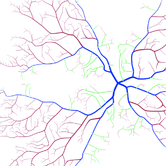

  

  Colour illustration of different types of vessels

  • left and right strong blood vessels (blue),

  • left/right wider weak blood vessel emerging from the left/right strong blood vessel (green),

  • other blood vessels (red).

The root of the branch tree is the point located at the centre of the optic nerve target. It creates one of the following branching points, and then generates the tree recursively so that each new branching point generates the following two branch points. Generation ends when the vessel’s width at the newly created point is ≤0. The properties of the following branch points are also calculated, and the design of the method of calculating some of them was based on the information published in [39].

The distance from the previous point d is calculated for the following two points according to the vessel width w_a at the current point as follows:

$$ d = \left\{ {\begin{array}{*{20}c} {rand\left( {0.15,\,0.05} \right)\,{\text{for}}\,w_{a} > 0.15} \\ {rand\left( {0.05,\,0.02} \right)\quad {\text{else}}} \\ \end{array} } \right.. $$

(4.1)

This has the consequence of the narrow blood vessels having more branches.

First, depending on the type of branch of the current point, the ratio is calculated to which the right and left successor are divided. If it is the current point Y-branch, the ratio of right and left successors is calculated as r: (1 – r), where r = rand (0.45, 0.55). In case of T-branching, it is 50% probability r = rand (0.95, 0.99), otherwise r = rand (0.01, 0.05).

If the current point is a part of the leftmost or rightmost strong blood vessel, this probability is altered in the T-branch, such that the weaker T-branch branches are generated towards the boundary of the quadrant. In the beginning, there is a 70% probability that the weaker vessel is generated towards the boundary of the quadrant. If this happens, this probability will decrease by 10% for the type of vessel (left or right); if not, the probability will increase by 10%.

The value of the vessel’s width is then calculated for both of the following branch points using their distance from the actual point, the vessel width at the current point, and the division ratio as follows:

$$ w_{r} = \left( {w_{a} \times \sqrt r } \right) - \left( {w_{a} \times \frac{{d_{r} }}{10}} \right) - \frac{{d_{r} }}{20}, $$

(4.2)

$$ w_{l} = \left( {w_{a} \times \sqrt {1 - r} } \right) - \left( {w_{a} \times \frac{{d_{l} }}{10}} \right) - \frac{{d_{l} }}{20}. $$

(4.3)

If the width of the calculated vessel at the next point is not positive, this point is marked as the vessel endpoint. If the calculated width is negative, the distance of that point from the previous point is adjusted to the width of the vessel, which at that point is equal to zero.

In other cases, it is decided whether the following point will be a Y-branch or a T-branch. One of the auxiliary features of a point is the probability of selecting the Y-Branch for its following branching points, that is, at the starting point, set to 20%. If the selected branch type of the next branch is the Y-branch, then this probability is set to 0% at this next point. If the T-branch is selected and the next point is the weaker T-branch of the current point, the probability for this next point is set to 40%. Otherwise, the probability is increased by 25%.

First, the position of the leftmost and rightmost points of thick blood vessels (type 1) is calculated, then it points the position of the left/right wider weak blood vessels resulting from vascular type 1 (type 2) and finally, the position of the other vessel (type 3). Within these types of vessels, the order of points in the calculation of the positions is given by the width of the vessel at a given point, with the positions of the wider vessels being counted first. Point positions are counted in this order because not all tree branch points generated will eventually be used.

When calculating the position of a particular branch point, the set of positions on which this point may be located is first determined. From the beginning, these are the positions around the previous branch point at the distance that this particular point has generated as a property. Then, depending on the direction of the vessel at the previous point, this set is limited by the interval of angles in which the position of the point may be. For each of the remaining positions, the weight of the position is calculated based on the deviation from the centre of the interval.

On the real images, the observed part of the retina is circular and the rest of square image is black. A majority of the right-hand portion of the image tends to see a smaller part of the retina in the shape of a semicircle or rectangle. This is to know where the picture is; for example, if it is not turned.

The generator allows you to choose which quadrant the mark will be in, and also whether the mark will have the shape of a semicircle or rectangle. The generated texture has a black colour and, depending on the coordinates, only the transparency of the texture changes.

4.5 Testing

We are now comparing the created synthetic retinal images with our ground truth. We use manually marked, real retinal images to create a density map, where there are the most bifurcation and crossing points. Using the same procedure, we want to automatically create a density map for synthetic retinal images and compare both results.

We developed the applications SW₁ and SW₂ (see Sect. 11.3.2). SW₁ was developed for manually marking blind spots, yellow spots and features, as well as determining their polar coordinates. We marked all retinal images via SW₁ one by one.

SW₂ was developed to estimate the number of feature points in different regions. SW₂ loaded all marked retinal images one by one and mapped polar coordinates of feature points to Cartesian coordinates. After that, SW₂ presented the intensity of occurring features in 5 × 5 pixels by a range of shades of grey. The darker shade represented higher occurrence of features, whereas the lighter shade represented lower occurrence.

Using the application described in the previous chapters, 1,000 images were generated in which the crossover and bifurcation were found. The occurrence frequencies were merged with the SW₂ described in Sect. 11.2.2 and graphically represented result seen in Fig. 11.34 left.

Fig. 11.34

(Left) Density occurrence of summarised real retinas; (right) density in synthetically generated retinas

It was then possible to visually compare the results of synthetic and real retinal images. In Fig. 11.34 right, there are visible features on the blind spot. It’s a side effect. On real retinas, there were no marked features inside the blind spot.

Figure 11.34 shows the summarised occurrences of crosses and bifurcations for real (left) and synthetic (right) retinal images. Picture (left) is marked manually and picture (right) is marked automatically. Both pictures are made up of about a thousand retinas. The shades’ range of the right picture is expanded because automated search for markers included features inside the blind spot. Features inside the blind spot in the left image were removed during manual labelling. Although the application generates blood vessels in the synthetic retina symmetrically, some similarities with the summation from the real retina can be traced.

The application is composed only of basic algorithms. As a result, there could be regular shapes seen in Fig. 11.34 right. We assume that, based on real retinas research, we can better specify the distribution of crossings and bifurcations in the model.

4.6 Generating Synthetic Images Via Neural Network

In another application, we first generate healthy images, where we can train algorithms for detection and extraction of the optical disc and fovea. Furthermore, we generate diseased retinal images with manifestations of ARMD and diabetes, e.g. haemorrhages, exudates. The neural network learns such images, which we have in the training set. At the moment, we only have images only for ARMD and diabetes; however, new images are stored in the database, i.e. it is possible to add new features representing new ophthalmologic diseases.

In biometric systems, it is often the case that a damaged image does not pass through the recognition. However, there is often not enough training data for detecting algorithms. Therefore, it is advisable to create large databases of synthetic meshes damaged by disease.

We have trained Generative Adversarial Networks (GANs) [40] to generate synthesised retinal images. A GANs-based retinal image synthesiser consists of two neural networks: a Generator (G) and a Discriminator (D). We have not used any extra information (such as blood vessel trees) to generate retinal images using GANs. However, we have emphasised maintaining a balance between the two competitors (i.e. G) and (D) during training. We have found that if this balance is not kept, G may end up generating only blurry retina images without high-level structures, such as blood vessel trees, optic discs, macula, etc.

Algorithm of GANs-based Retinal Synthesiser is as follows:

• For k times

  • Prepare a mini-batch of retinal images $\left\{ {\left( {x,\hat{x}} \right)_{i = 1}^{m} } \right\}^{kn}$ where m is the mini-batch size.

  • Update D using $\left\{ {\left( {x,\hat{x}} \right)_{i = 1}^{m} } \right\}^{kn}$.

• For r times

  • Prepare a mini-batch of noise vectors, $\left\{ {\left( z \right)_{i = 1}^{m} } \right\}^{rn}$.

  • Update G using $\left\{ {\left( z \right)_{i = 1}^{m} } \right\}^{rn}$.

We have used 1,200 images from the public database Messidor [18]. These images were acquired by three ophthalmologic departments using a colour video 3CCD camera on a Topcon TRC NW6 non-mydriatic retinograph with a 45-degree field of view. The images were captured using 8 bits per colour plane. Among these 1,200 images, 588 images were 960 × 1440, 400 images were 1488 × 2240 and 212 images were 1536 × 2304. In our experiments, we resized all of the images to the same size (i.e. 256 × 256) by bicubic interpolation.

We have followed the deep convolutional neural network-based architecture suggested in [41] with minor modifications. Table 2 shows the model architecture for 256 × 256-sized images. The mini-batch size was set to 32 (i.e. m = 32). Noise vectors were drawn from the uniform distribution. As a loss function, binary cross-entropy was used. As an optimiser, RMSProp with a learning rate of 0:0001 and a decay of 3e⁻⁸ was used. The dropout value was set to 0:5. For batch normalisation, momentum was set to 0:5 instead of default value 0:99. For LeakyReLU, it was set to 0.2 instead of the default value of 0:3. For all convolutional and transposed convolutional layers, stride = 2, kernel size = 5 and padding = same was used. l2 regularisation was applied only for weights and biases of the transposed convolutional layers. For all other settings, the default values of Tensor Flow’s Keras API were used.

After training, the generator is used to generate synthesised retinal images from noise vectors. The Structural SIMilarity (SSIM) measure shows how similar the synthesised images are to the training data. SSM = 0 means there is no similarity and SSIM = 1 means that two images are the same. You can see some achieved results from this GAN generator of synthetic retinal images in Figs. 11.35 and 11.36.

Fig. 11.35

Comparison of synthetic image and the closest training image from the database

Fig. 11.36

Examples of generated synthetic retinal images

A sample database of generated images is available at https://strade.fit.vutbr.cz/databases/synthetic_retina.

The database is separated into two parts: healthy images and disease-affected images, which is especially diabetes and ARMD.

References

Barajas H (2015) Atlas of the human eye: anatomy and biometrics. Palibrio, p 74. ISBN 978-1506510330
Snell RS, Lemp MA (2013) Clinical anatomy of the eye, 2nd edn. Wiley-Blackwell. ISBN 978-0632043446
Bergmüller T, Christopoulos E, Schnöll M, Uhl A (2015) Recompression effects in iris segmentation. In: Proceedings of the 8th IAPR/IEEE international conference on biometrics (ICB’15). Phuket, Thailand, pp 1–8
Nguyen K et al (2018) Iris recognition with off-the-shelf CNN features: a deep learning perspective. IEEE Access 6:18848–18855
Trokielewicz M, Czajka A, Maciejewicz P (2019) Iris recognition after death. IEEE Trans Inf Forensics Secur 14(6):1501–1514
Goldstein I, Simon C (1935) A new scientific method of identification. N Y State J Med 35
Tower P (1955) The fundus oculi in monozygotic twins: report of six pairs of identical twins. AMA Arch Ophthalmol 54:225–239
Farzin H, Abrishami-Moghaddam H, Moin MS (2008) A novel retinal identification system. EURASIP J Adv Signal Process Hindawi 2008:10. https://doi.org/10.1155/2008/280635
Hill RB (1996) Retina identification. In: Biometrics: personal identification in networked society. Springer, New York, pp 123–141
Timberlake GT, Kennedy M (2005) The direct ophthalmoscope—how it works and how to use it. University of Kansas, p 39. Available online on http://web.media.mit.edu/~raskar/Eye/TheDirectOphthalmoscope.pdf
Hill RB (1986) U.S. Patent 4,620,318. http://www.freepatentsonline.com/4620318.pdf
Arndt JH (1990) U.S. Patent 4,923,297. http://www.freepatentsonline.com/4923297.pdf
Johnson JC, Hill RB U.S. Patent 5,532,771. http://www.freepatentsonline.com/5532771.pdf
Fuhrmann T, Hämmerle-Uhl J, Uhl A (2009) Usefulness of retina codes in biometrics. In: Advances in image and video technology, 3rd Pacific Rim symposium, Japan, Springer LNCS 5414. ISSN 0302-9743
Arakala A, Culpepper JS, Jeffers J, Turpin A, Boztas S, Horadami KJ, McKendrick AM Entropy of the retina template. RMIT University, Melbourne, Australia
Shih HP 2008 Two algorithms for maximum and minimum weighted bipartite matching. Department of Computer Science and Information Engineering National Taiwan University
Carmona E, Rincón M, García-Feijoo J, Martínez-de-la Casa J (2008) Identification of the optic nerve head with genetic algorithms. Artif Intell Med 43:243–259
Decencière E, Zhang X, Cazuguel G, Lay B, Cochener B, Trone C, Gain P, Ordonez R, Massin P, Erginay A, Charton B, Klein JC (2014) Feedback on a publicly distributed database: the messidor database. Image Anal Stereol 33(3):231–234
Kohler T, Budai A, Kraus M, Odstrčilík J, Michelson G, Hornegger J (2013) Automatic no-reference quality assessment for retinal fundus images using vessel segmentation. In: 26th IEEE international symposium on computer-based medical systems. pp 95–100
Ortega M, Penedo MG, Rouco J, Barreira N, Carreira MJ (2009) Retinal verification using a feature points based biometric pattern. EURASIP J Adv Signal Proc 2009. Article ID 235746:13 pp
Albert DM, Miller JW et al (2008) Principles and practice of ophthalmology, 3rd edn. ISBN 978-1-4160-0016-7
Ryan SJ (2006) Retina. Elsevier Mosby. ISBN 0323043232
Diagnosis and classification of diabetes mellitus. Diabetes Care, American Diabetes Association, Issue 33, 2010, pp 62–69. https://doi.org/10.2337/dc10-s062
Scanlon PH, Wilkinson CP, Aldington SJ, Matthews DR (2009) A practical manual of diabetic retinopathy management. Wiley-Blackwell. ISBN 978-1-405-17035-2
Sosna T (2016) Diabetická retinopatie (Diabetic retinopathy), 2nd edn. Prague, Axonite CZ. ISBN 9788088046059
Cavallotti CAP, Cerulli L (2008) Age-related changes of the human eye. Humana Press, p 400
Kolář P (2008) Věkem podmíněná makulární degenerace (Aged-related macular degeneration), 1st edn. Prague, Grada. ISBN 9788024726052
Kanski JJ (2007) Clinical ophthalmology—a systematic approach, 6th edn. Elsevier, p. 942. ISBN 978-0-08-044969-2
Ernest J. Makulární degenerace (Macular degeneration). Prague, Mladá fronta, 1st Edition, 2010, ISBN 9788020423634
Pašta J (2017) Základy očního lékařství (Basics of ophthalmology). Charles University, Karolinum, Prague. ISBN 978-80-246-2460-0
Staal J, Abramoff M, Niemeijer M (2004) Ridge based vessel segmentation in color images of the retina. IEEE Trans Med Imaging 23(4):501–509
Daugman J (2006) Probing the uniqueness and randomness of iriscodes: results from 200 billion iris pair comparisons. Proc IEEE 94(11):1927–1935
Adler A, Youmaran R, Loyka S (2006) Towards a measure of biometric information. In: Canadian conference on electrical and computer engineering, (CCECE’06). pp 210–213
Nautsch A, Rathgeb C, Saeidi R, Busch C (2015) Entropy analysis of I-vector feature spaces in duration-sensitive speaker recognition. In: 40th IEEE ICASSP conference, 19–24 April 2015. Brisbane, Australia
Decencière E, Cazuguel G, Zhang X, Thibault G, Klein JC, Meyer F, Marcotegui B, Quellec G, Lamard M, Danno R, Elie D, Massin P, Viktor Z, Erginay A, La B, Chabouis A (2013) Teleophta: machine learning and image processing methods for teleophthalmology. IRBM, Elsevier Masson 34(2):196–203
Pres M (2016) Bifurcation localization in retina images. MSc thesis, supervised by: Lukas Semerad, Brno University of Technology, Faculty of Information Technology, Czech Republic
Mortenson ME (1999) Mathematics for computer graphics applications. Industrial Press Inc., p 264. ISBN 9780831131111
Zamir M, Medeiros JA, Cunningham TK (1979) Arterial bifurcations in the human retina. J Gen Physiol 74(4):537–548
Goodfellow IJ, Pouget-Abadie J, Mirza M, Xu B, Warde-Farley D, Ozair S, Courville AC, Bengio Y (2014) Generative adversarial networks. CoRR, abs/1406.2661
Radford A, Metz L, Chintala S (2015) Unsupervised representation learning with deep convolutional generative adversarial networks. CoRR, abs/1511.06434
Anatomy and physiology, Connexions Web site. http://cnx.org/content/col11496/1.6/
Optimis Fusion. http://www.askin.cz/prednesegmentove/. Accessed 6 June 2018
Kowa VX-20. http://dfv.com.au/products/diagnostic/diagnostic-imaging/kowa-vx-20-mydriatic-non-mydriatic-integrated-fundus-camera/. Accessed 6 June 2018
https://cryptologicfoundation.org/visit/museum/acquisitions/acquisitionarchivessection/individualequipmentitems/rfsignalgenerator.html. Accessed 11 June 2018
http://retinagallery.com/displayimage.php?album=228&pid=2596#top_display_media
Nugroho HA et al (2015) Automated microaneurysms (MAs) detection in digital colour fundus images using matched filter. In: 2015 international conference on computer, control, informatics and its applications (IC3INA). pp 104–108
Dalton M (2012) Evaluating the risks of retinal detachment in cataract patients. Eyeworld. https://www.eyeworld.org/article-evaluating-the-risks-of-retinal
Vlhká forma s edémem (Wet form with edema). Prague, Mladá frona. https://img.mf.cz/062/617/c.jpg. Accessed 25 June 2018
Retina Image Bank®. https://imagebank.asrs.org/file/1428/lacquer-cracks
Acknowledgements
This work was supported by The Ministry of Education, Youth and Sports of the Czech Republic from the National Programme of Sustainability (NPU II); project “IT4Innovations excellence in science—LQ1602” and the BUT project “Secure and Reliable Computer Systems”, FIT-S-17-4014.
Author information
Authors and Affiliations
Corresponding author
Editor information
Editors and Affiliations
Rights and permissions
Open Access This chapter is licensed under the terms of the Creative Commons Attribution 4.0 International License (http://creativecommons.org/licenses/by/4.0/), which permits use, sharing, adaptation, distribution and reproduction in any medium or format, as long as you give appropriate credit to the original author(s) and the source, provide a link to the Creative Commons license and indicate if changes were made.
The images or other third party material in this chapter are included in the chapter's Creative Commons license, unless indicated otherwise in a credit line to the material. If material is not included in the chapter's Creative Commons license and your intended use is not permitted by statutory regulation or exceeds the permitted use, you will need to obtain permission directly from the copyright holder.
Copyright information
© 2020 The Author(s)
About this chapter
Cite this chapter
Semerád, L., Drahanský, M. (2020). Retinal Vascular Characteristics. In: Uhl, A., Busch, C., Marcel, S., Veldhuis, R. (eds) Handbook of Vascular Biometrics. Advances in Computer Vision and Pattern Recognition. Springer, Cham. https://doi.org/10.1007/978-3-030-27731-4_11
Download citation
DOI: https://doi.org/10.1007/978-3-030-27731-4_11
Published:
Publisher Name: Springer, Cham
Print ISBN: 978-3-030-27730-7
Online ISBN: 978-3-030-27731-4
eBook Packages: Computer ScienceComputer Science (R0)