Measuring Masking Fault-Tolerance

Fault-tolerance allows for the construction of systems that are able to overcome the occurrence of faults during their execution. Examples of fault-tolerant systems can be found everywhere: communication protocols, hardware circuits, avionic systems, cryptographic currencies, etc. So, the increasing relevance of critical software in everyday life has led to a renewed interest in the automatic verification of fault-tolerant properties. However, one of the main difficulties when reasoning about these kinds of properties is given by their quantitative nature, which is true even for non-probabilistic systems. A simple example is given by the introduction of redundancy in critical systems. This is, by far, one of the most used techniques in fault-tolerance. In practice, it is well-known that adding more redundancy to a system increases its reliability. Measuring this increment is a central issue for evaluating fault-tolerant software, protocols, etc. On the other hand, the formal characterization of fault-tolerant properties could be an involving task, usually these properties are encoded using ad-hoc mechanisms as part of a general design.

The usual flow for the design and verification of fault-tolerant systems consists in defining a nominal model (i.e., the “fault-free” or “ideal” program) and afterwards extending it with faulty behaviors that deviate from the normal behavior prescribed by the nominal model. This extended model represents the way in which the system operates under the occurrence of faults. There are different ways of extending the nominal model, the typical approach is fault injection [20, 21], that is, the automatic introduction of faults into the model. An important property that any extended model has to satisfy is the preservation of the normal behavior under the absence of faults. In [11], we proposed an alternative formal approach for dealing with the analysis of fault-tolerance. This approach allows for a fully automated analysis and appropriately distinguishes faulty behaviors from normal ones. Moreover, this framework is amenable to fault-injection. In that work, three notions of simulation relations are defined to characterize masking, nonmasking, and failsafe fault-tolerance, as originally defined in [15].

During the last decade, significant progress has been made towards defining suitable metrics or distances for diverse types of quantitative models including real-time systems [19], probabilistic models [12], and metrics for linear and branching systems [6, 8, 18, 23, 29]. Some authors have already pointed out that these metrics can be useful to reason about the robustness of a system, a notion related to fault-tolerance. Particularly, in [6] the traditional notion of simulation relation is generalized and three different simulation distances between systems are introduced, namely correctness, coverage, and robustness. These are defined using quantitative games with discounted-sum and mean-payoff objectives.

In this paper we introduce a notion of fault-tolerance distance between labelled transition systems. Intuitively, this distance measures the degree of fault-tolerance exhibited by a candidate system. As it was mentioned above, there exist different levels of fault-tolerance, we restrict ourselves to the analysis of masking fault-tolerance because it is often classified as the most benign kind of fault-tolerance and it is a highly desirable property for critical systems. Roughly speaking, a system is masking fault-tolerant when it is able to completely mask the faults, not allowing these faults to have any observable consequences for the users. Formally, the system must preserve both the safety and liveness properties of the nominal model [15]. In contrast to the robustness distance defined in [6], which measures how many unexpected errors are tolerated by the implementation, we consider a specific collection of faults given in the implementation and measure how many faults are tolerated by the implementation in such a way that they can be masked by the states. We also require that the normal behavior of the specification has to be preserved by the implementation when no faults are present. In this case, we have a bisimulation between the specification and the non-faulty behavior of the implementation. Otherwise, the distance is 1. That is, \(\delta _{m}(N,I)=1\) if and only if the nominal model N and \(I\backslash F\) are not bisimilar, where \(I\backslash F\) behaves like the implementation I where all actions in F are forbidden (\(\backslash \) is Milner’s restriction operator). Thus, we effectively distinguish between the nominal model and its fault-tolerant version and the set of faults taken into account.

In order to measure the degree of masking fault-tolerance of a given system, we start characterizing masking fault-tolerance via simulation relations between two systems as defined in [11]. The first one acting as a specification of the intended behavior (i.e., nominal model) and the second one as the fault-tolerant implementation (i.e., the extended model with faulty behavior). The existence of a masking relation implies that the implementation masks the faults. Afterwards, we introduce a game characterization of masking simulation and we enrich the resulting games with quantitative objectives to define the notion of masking fault-tolerance distance, where the possible values of the game belong to the interval [0, 1]. The fault-tolerant implementation is masking fault-tolerant if the value of the game is 0. Furthermore, the bigger the number, the farther the masking distance between the fault-tolerant implementation and the specification. Accordingly, a bigger distance remarkably decreases fault-tolerance. Thus, for a given nominal model N and two different fault-tolerant implementations \(I_1\) and \(I_2\), our distance ensures that \(\delta _{m}(N,I_1)<\delta _{m}(N,I_2)\) whenever \(I_1\) tolerates more faults than \(I_2\). We also provide a weak version of masking simulation, which makes it possible to deal with complex systems composed of several interacting components. We prove that masking distance is a directed semimetric, that is, it satisfies two basic properties of any distance, reflexivity and the triangle inequality.

Finally, we have implemented our approach in a tool that takes as input a nominal model and its fault-tolerant implementation and automatically compute the masking distance between them. We have used this tool to measure the masking tolerance of multiple instances of several case studies such as a redundant cell memory, a variation of the dining philosophers problem, the bounded retransmission protocol, N-Modular-Redundancy, and the Byzantine generals problem. These are typical examples of fault-tolerant systems.

The remainder of the paper is structured as follows. In Sect. 2, we introduce preliminaries notions used throughout this paper. We present in Sect. 3 the formal definition of masking distance build on quantitative simulation games and we also prove its basic properties. We describe in Sect. 4 the experimental evaluation on some well-known case studies. In Sect. 5 we discuss the related work. Finally, we discuss in Sect. 6 some conclusions and directions for further work. Full details and proofs can be found in [5].

Let us introduce some basic definitions and results on game theory that will be necessary across the paper, the interested reader is referred to [2].

A transition system (TS) is a tuple \(A =\langle S, \varSigma , E, s_0\rangle \), where S is a finite set of states, \(\varSigma \) is a finite alphabet, \(E \subseteq S \times \varSigma \times S\) is a set of labelled transitions, and \(s_0\) is the initial state. In the following we use \(s \xrightarrow {e} s' \in E\) to denote \((s,e,s') \in E\). Let |S| and |E| denote the number of states and edges, respectively. We define \(post(s) = \{s' \in S \mid s \xrightarrow {e} s' \in E\}\) as the set of successors of s. Similarly, \(pre(s') = \{s \in S \mid s \xrightarrow {e} s' \in E \}\) as the set of predecessors of \(s'\). Moreover, \(post^{*}(s)\) denotes the states which are reachable from s. Without loss of generality, we require that every state s has a successor, i.e., \(\forall s \in S : post(s) \ne \emptyset \). A run in a transition system A is an infinite path \(\rho = \rho _0 \sigma _0 \rho _1 \sigma _1 \rho _2 \sigma _2 \dots \in (S \cdot \varSigma )^{w}\) where \(\rho _0 = s_0\) and for all i, \(\rho _i \xrightarrow {\sigma _i} \rho _{i+1} \in E\). From now on, given a tuple \((x_0,\dots ,x_n)\), we denote \(x_i\) by \(\text{ pr }_{i}((x_0,\dots ,x_n))\).

A game graph G is a tuple \(G = \langle S, S_1, S_2, \varSigma , E, s_0 \rangle \) where S, \(\varSigma \), E and \(s_0\) are as in transition systems and \((S_1, S_2)\) is a partition of S. The choice of the next state is made by Player 1 (Player 2) when the current state is in \(S_1\) (respectively, \(S_2\)). A weighted game graph is a game graph along with a weight function \(v^G\) from E to \(\mathbb {Q}\). A run in the game graph G is called a play. The set of all plays is denoted by \(\varOmega \).

Given a game graph G, a strategy for Player 1 is a function \(\pi : (S \cdot \varSigma )^{*} S_1 \rightarrow \varSigma \times S\) such that for all \(\rho _0 \sigma _0 \rho _1 \sigma _1 \dots \rho _i~\in ~(S \cdot \varSigma )^{*} S_1\), we have that if \(\pi (\rho _0 \sigma _0 \rho _1 \sigma _1 \dots \rho _i) = (\sigma , \rho )\), then \(\rho _i \xrightarrow {\sigma } \rho \in E\). A strategy for Player 2 is defined in a similar way. The set of all strategies for Player p is denoted by \(\varPi _{p}\). A strategy for player p is said to be memoryless (or positional) if it can be defined by a mapping \(f:S_p \rightarrow E\) such that for all \(s \in S_p\) we have that \(\text{ pr }_{0}(f(s))=s\), that is, these strategies do not need memory of the past history. Furthermore, a play \(\rho _0 \sigma _0 \rho _1 \sigma _1 \rho _2 \sigma _2 \dots \) conforms to a player p strategy \(\pi \) if \(\forall i \ge 0: (\rho _i \in S_p) \Rightarrow (\sigma _{i}, \rho _{i+1}) = \pi (\rho _0 \sigma _0 \rho _1 \sigma _1 \dots \rho _i)\). The outcome of a Player 1 strategy \(\pi _{1}\) and a Player 2 strategy \(\pi _2\) is the unique play, named \(out(\pi _1, \pi _2)\), that conforms to both \(\pi _1\) and \(\pi _2\).

A game is made of a game graph and a boolean or quantitative objective. A boolean objective is a function \(\varPhi : \varOmega \rightarrow \{0, 1\}\) and the goal of Player 1 in a game with objective \(\varPhi \) is to select a strategy so that the outcome maps to 1, independently what Player 2 does. On the contrary, the goal of Player 2 is to ensure that the outcome maps to 0. Given a boolean objective \(\varPhi \), a play \(\rho \) is winning for Player 1 (resp. Player 2) if \(\varPhi (\rho ) = 1\) (resp. \(\varPhi (\rho ) = 0\)). A strategy \(\pi \) is a winning strategy for Player p if every play conforming to \(\pi \) is winning for Player p. We say that a game with boolean objective is determined if some player has a winning strategy, and we say that it is memoryless determined if that winning strategy is memoryless. Reachability games are those games whose objective functions are defined as \(\varPhi (\rho _0 \sigma _0 \rho _1 \sigma _1 \rho _2 \sigma _2 \dots ) = (\exists i : \rho _i \in V)\) for some set \(V \subseteq S\), a standard result is that reachability games are memoryless determined.

A quantitative objective is given by a payoff function \(f: \varOmega \rightarrow \mathbb {R}\) and the goal of Player 1 is to maximize the value f of the play, whereas the goal of Player 2 is to minimize it. For a quantitative objective f, the value of the game for a Player 1 strategy \(\pi _1\), denoted by \(v_1(\pi _1)\), is defined as the infimum over all the values resulting from Player 2 strategies, i.e., \(v_1(\pi _1) = \inf _{\pi _2 \in \varPi _2} f(out(\pi _1, \pi _2))\). The value of the game for Player 1 is defined as the supremum of the values of all Player 1 strategies, i.e., \(\sup _{\pi _1 \in \varPi _1} v_1(\pi _1)\). Analogously, the value of the game for a Player 2 strategy \(\pi _2\) and the value of the game for Player 2 are defined as \(v_2(\pi _2) = \sup _{\pi _1 \in \varPi _1} f(out(\pi _1, \pi _2))\) and \(\inf _{\pi _2 \in \varPi _2} v_2(\pi _2)\), respectively. We say that a game is determined if both values are equal, that is: \(\sup _{\pi _1 \in \varPi _1} v_1(\pi _1) = \inf _{\pi _2 \in \varPi _2} v_2(\pi _2)\). In this case we denote by \(val(\mathcal {G})\) the value of game \(\mathcal {G}\). The following result from [24] characterizes a large set of determined games.

We start by defining masking simulation. In [11], we have defined a state-based simulation for masking fault-tolerance, here we recast this definition using labelled transition systems. First, let us introduce some concepts needed for defining masking fault-tolerance. For any vocabulary \(\varSigma \), and set of labels \(\mathcal {F} = \{F_0, \dots , F_n\}\) not belonging to \(\varSigma \), we consider \(\varSigma _{\mathcal {F}}= \varSigma \cup \mathcal {F}\), where \(\mathcal {F} \cap \varSigma = \emptyset \). Intuitively, the elements of \(\mathcal {F}\) indicate the occurrence of a fault in a faulty implementation. Furthermore, sometimes it will be useful to consider the set \(\varSigma ^i = \{ e^i \mid e \in \varSigma \}\), containing the elements of \(\varSigma \) indexed with superscript i. Moreover, for any vocabulary \(\varSigma \) we consider \(\varSigma _{M}= \varSigma \cup \{M\}\), where \(M \notin \varSigma \), intuitively, this label is used to identify masking transitions.

Given a transition system \(A = \langle S, \varSigma , E, s_0 \rangle \) over a vocabulary \(\varSigma \), we denote \(A^M = \langle S, \varSigma _{M}, E^M, s_0 \rangle \) where \(E^M = E \cup \{s \xrightarrow {M} s \mid s \in S\}\).

3.2 Weak Masking Simulation

For analysing nontrivial systems a weak version of masking simulation relation is needed, the main idea is that a weak masking simulation abstracts away from internal behaviour, which is modeled by a special action \(\tau \). Note that internal transitions are common in fault-tolerance: the actions performed as part of a fault-tolerant procedure in a component are usually not observable by the rest of the system.

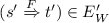
The weak transition relations \({\Rightarrow } \subseteq S \times (\varSigma \cup \{\tau \} \cup \{M\} \cup \mathcal {F}) \times S\), also denoted as \(E_W\), considers the silent step \(\tau \) and is defined as follows:

Open image in new window

The symbol \(\circ \) stands for composition of binary relations and \((\xrightarrow {\tau })^{*}\) is the reflexive and transitive closure of the binary relation \(\xrightarrow {\tau }\).

Intuitively, if \(e \notin \{\tau ,M\}\cup \mathcal {F}\), then Open image in new window means that there is a sequence of zero or more \(\tau \) transitions starting in s, followed by one transition labelled by e, followed again by zero or more \(\tau \) transitions eventually reaching \(s'\). Open image in new window states that s can transition to \(s'\) via zero or more \(\tau \) transitions. In particular, Open image in new window for every s. For the case in which \(e\in \{M\}\cup \mathcal {F}\), Open image in new window is equivalent to Open image in new window and hence no \(\tau \) step is allowed before or after the e transition.

Definition 2

Let \(A =\langle S, \varSigma , E, s_0\rangle \) and \(A' =\langle S', \varSigma _{\mathcal {F}}, E', s_0' \rangle \) be two transition systems with \(\varSigma \) possibly containing \(\tau \). \(A'\) is weak masking fault-tolerant with respect to A if there is a relation \(\mathbin {\mathbf {M}}\subseteq S \times S'\) between \(A^M\) and \(A'\) such that:

1. (A)

   \(s_0 \mathrel {\mathbin {\mathbf {M}}} s'_0\)

    
2. (B)
   for all \(s \in S, s' \in S'\) with \(s \mathrel {\mathbin {\mathbf {M}}} s'\) and all \(e \in \varSigma \cup \{\tau \}\) the following holds:

   1. (1)

      if \((s \xrightarrow {e} t) \in E\) then Open image in new window ;

       
   2. (2)

      if \((s' \xrightarrow {e} t') \in E'\) then Open image in new window ;

       
   3. (3)

      if \((s' \xrightarrow {F} t') \in E'\) for some \(F \in \mathcal {F}\) then \(\exists \; t \in S: (s \xrightarrow {M} t \in E \wedge t \mathrel {\mathbin {\mathbf {M}}} t').\)

       
    

If such relation exists, we say that \(A'\) is a weak masking fault-tolerant implementation of A, denoted by \(A \preceq ^w_{m}A'\).

The following theorem makes a strong connection between strong and weak masking simulation. It states that weak masking simulation becomes strong masking simulation whenever transition \(\xrightarrow {}\) is replaced by Open image in new window in the original automata.

Theorem 2

Let \(A =\langle S, \varSigma , E, s_0\rangle \) and \(A' =\langle S', \varSigma _{\mathcal {F}}, E', s_0' \rangle \). \(\mathbin {\mathbf {M}}\subseteq S \times S'\) between \(A^M\) and \(A'\) is a weak masking simulation if and only if:

1. (A)

   \(s_0 \mathrel {\mathbin {\mathbf {M}}} s'_0\), and

    
2. (B)
   for all \(s \in S, s' \in S'\) with \(s \mathrel {\mathbin {\mathbf {M}}} s'\) and all \(e \in \varSigma \cup \{\tau \}\) the following holds:

   1. (1)

      if Open image in new window then Open image in new window ;

       
   2. (2)

      if Open image in new window then Open image in new window ;

       
   3. (3)

      if Open image in new window for some \(F \in \mathcal {F}\) then Open image in new window

       
    

The proof of this is straightforward following the same ideas of Milner in [25].

A natural way to check weak bisimilarity is to saturate the transition system [14, 25] and then check strong bisimilarity on the saturated transition system. Similarly, Theorem 2 allows us to compute weak masking simulation by reducing this problem to compute strong masking simulation. Note that Open image in new window can be alternatively defined by:

Open image in new window

As a running example, we consider a memory cell that stores a bit of information and supports reading and writing operations, presented in a state-based form in [11]. A state in this system maintains the current value of the memory cell (\(m=i\), for \(i=0,1\)), writing allows one to change this value, and reading returns the stored value. Obviously, in this system the result of a reading depends on the value stored in the cell. Thus, a property that one might associate with this model is that the value read from the cell coincides with that of the last writing performed in the system.

A potential fault in this scenario occurs when a cell unexpectedly loses its charge, and its stored value turns into another one (e.g., it changes from 1 to 0 due to charge loss). A typical technique to deal with this situation is redundancy: use three memory bits instead of one. Writing operations are performed simultaneously on the three bits. Reading, on the other hand, returns the value that is repeated at least twice in the memory bits; this is known as voting.

We take the following approach to model this system. Labels \(\text {W}_0, \text {W}_1, \text {R}_0,\) and \(\text {R}_1\) represent writing and reading operations. Specifically, \(\text {W}_0\) (resp. \(\text {W}_1\)): writes a zero (resp. one) in the memory. \(\text {R}_0\) (resp. \(\text {R}_1\)): reads a zero (resp. one) from the memory. Figure 1 depicts four transition systems. The leftmost one represents the nominal system for this example (denoted as A). The second one from the left characterizes the nominal transition system augmented with masking transitions, i.e., \(A^M\). The third and fourth transition systems are fault-tolerant implementations of A, named \(A'\) and \(A''\), respectively. Note that \(A'\) contains one fault, while \(A''\) considers two faults. Both implementations use triple redundancy; intuitively, state \(\text {t}_0\) contains the three bits with value zero and \(\text {t}_1\) contains the three bits with value one. Moreover, state \(\text {t}_2\) is reached when one of the bits was flipped (either 001, 010 or 100). In \(A''\), state \(\text {t}_3\) is reached after a second bit is flipped (either 011 or 101 or 110) starting from state \(\text {t}_0\). It is straightforward to see that there exists a relation of masking fault-tolerance between \(A^M\) and \(A'\), as it is witnessed by the relation \(\mathbin {\mathbf {M}}= \{(\text {s}_0, \text {t}_0), (\text {s}_1, \text {t}_1), (\text {s}_0, \text {t}_2)\}\). It is a routine to check that \(\mathbin {\mathbf {M}}\) satisfies the conditions of Definition 1. On the other hand, there does not exist a masking relation between \(A^M\) and \(A''\) because state \(\text {t}_3\) needs to be related to state \(\text {s}_0\) in any masking relation. This state can only be reached by executing faults, which are necessarily masked with M-transitions. However, note that, in state \(\text {t}_3\), we can read a 1 (transition \(\text {t}_3 \xrightarrow {\text {R}_1} \text {t}_3\)) whereas, in state \(\text {s}_0\), we can only read a 0.

Open image in new window

3.3 Masking Simulation Game

We define a masking simulation game for two transition systems (the specification of the nominal system and its fault-tolerant implementation) that captures masking fault-tolerance. We first define the masking game graph where we have two players named by convenience the refuter (\(R\)) and the verifier (\(V\)).

Definition 3

Let \(A=\langle S, \varSigma , E, s_0\rangle \) and \(A'=\langle S', \varSigma _{\mathcal {F}}, E_W', s'_0 \rangle \). The strong masking game graph \(\mathcal {G}_{A^M,A'} = \langle S^G, S_R, S_V, \varSigma ^G, E^G, {s_0}^G \rangle \) for two players is defined as follows:

• \(\varSigma ^G = \varSigma _{M}\cup \varSigma _{\mathcal {F}}\)

• \(S^G = (S \times ( \varSigma _{M}^1 \cup \varSigma _{\mathcal {F}}^2 \cup \{\#\}) \times S' \times \{ R, V \}) \cup \{s_{err}\}\)

• The initial state is \(s_0^G = \langle s_0, \#, s'_0, R \rangle \), where the refuter starts playing

• The refuter’s states are \(S_R = \{ (s, \#, s', R) \mid s \in S \wedge s' \in S' \} \cup \{s_{err}\}\)

• The verifier’s states are \(S_V = \{ (s, \sigma , s', V) \mid s \in S \wedge s' \in S' \wedge \sigma \in \varSigma ^G\setminus \{M\}\}\)

and \(E^G\) is the minimal set satisfying:

• \(\{ (s, \#, s', R) \xrightarrow {\sigma } (t, \sigma ^{1}, s', V) \mid \exists \;\sigma \in \varSigma : s \xrightarrow {\sigma } t \in E \} \subseteq E^G\),

• \(\{ (s, \#, s', R) \xrightarrow {\sigma } (s, \sigma ^{2}, t', V) \mid \exists \;\sigma \in \varSigma _{\mathcal {F}}: s' \xrightarrow {\sigma } t' \in E' \} \subseteq E^G\),

• \(\{ (s, \sigma ^2, s', V) \xrightarrow {\sigma } (t, \#, s', R) \mid \exists \;\sigma \in \varSigma : s \xrightarrow {\sigma } t \in E \} \subseteq E^G\),

• \(\{ (s, \sigma ^1, s', V) \xrightarrow {\sigma } (s, \#, t', R) \mid \exists \;\sigma \in \varSigma : s' \xrightarrow {\sigma } t' \in E' \} \subseteq E^G\),

• \(\{ (s, F^2, s', V) \xrightarrow {M} (t, \#, s', R) \mid \exists \;s \xrightarrow {M} t \in E^M \} \subseteq E^G\), for any \(F \in \mathcal {F}\)

• If there is no outgoing transition from some state s then transitions \(s \xrightarrow {\sigma } s_{err}\) and \(s_{err}\xrightarrow {\sigma } s_{err}\) for every \(\sigma \in \varSigma \), are added.

The intuition of this game is as follows. The refuter chooses transitions of either the specification or the implementation to play, and the verifier tries to match her choice, this is similar to the bisimulation game [28]. However, when the refuter chooses a fault, the verifier must match it with a masking transition (M). The intuitive reading of this is that the fault-tolerant implementation masked the fault in such a way that the occurrence of this fault cannot be noticed from the users’ side. \(R\) wins if the game reaches the error state, i.e., \(s_{err}\). On the other hand, \(V\) wins when \(s_{err}\) is not reached during the game. (This is basically a reachability game [26]).

A weak masking game graph \(\mathcal {G}^W_{A^M,A'}\) is defined in the same way as the strong masking game graph in Definition 3, with the exception that \(\varSigma _{M}\) and \(\varSigma _{\mathcal {F}}\) may contain \(\tau \), and the set of labelled transitions (denoted as \(E_W^G\)) is now defined using the weak transition relations (i.e., \(E_W\) and \(E_W'\)) from the respective transition systems.

Figure 2 shows a part of the strong masking game graph for the running example considering the transition systems \(A^M\) and \(A''\). We can clearly observe on the game graph that the verifier cannot mimic the transition \((s_0, \#, t_3, R) \xrightarrow {R_1^2} (s_0, R_1^2, t_3, V)\) selected by the refuter which reads a 1 at state \(t_3\) on the fault-tolerant implementation. This is because the verifier can only read a 0 at state \(s_0\). Then, the \(s_{err}\) is reached and the refuter wins.

As expected, there is a strong masking simulation between A and \(A'\) if and only if the verifier has a winning strategy in \(\mathcal {G}_{A^M,A'}\).

Theorem 3

Let \(A=\langle S, \varSigma , E, s_0\rangle \) and \(A'=\langle S', \varSigma _{\mathcal {F}}, E', s_0' \rangle \). \(A \preceq _{m}A'\) iff the verifier has a winning strategy for the strong masking game graph \(\mathcal {G}_{A^M,A'}\).

By Theorems 2 and 3, the result replicates for weak masking game.

Theorem 4

Let \(A=\langle S, \varSigma \cup \{\tau \}, E, s_0\rangle \) and \(A'=\langle S', \varSigma _{\mathcal {F}}\cup \{\tau \}, E', s_0' \rangle \). \(A \preceq ^w_{m}A'\) iff the verifier has a winning strategy for the weak masking game graph \(\mathcal {G}^W_{A^M,A'}\).

Using the standard properties of reachability games we get the following property.

Theorem 5

For any A and \(A'\), the strong (resp. weak) masking game graph \(\mathcal {G}_{A^M, A'}\) (resp. \(\mathcal {G}^W_{A^M, A'}\)) can be determined in time \(O(|E^G|)\) (resp. \(O(|E_W^G|)\)).

Open image in new window

The set of winning states for the refuter can be defined in a standard way from the error state [26]. We adapt ideas in [26] to our setting. For \(i,j\ge 0\), sets \(U^j_i\) are defined as follows:

$$\begin{aligned} U^0_i =&U^j_0 = \emptyset , \\ U_1^1 =&\{s_{err}\}, {}\nonumber \end{aligned}$$

(1)

$$\begin{aligned} U_{i+1}^{j+1}&= \{v' \mid v' \in S_R \wedge post(v') \cap U_{i+1}^j \ne \emptyset \} \\&\textstyle {}\cup \{v' \mid v' \in S_V \wedge post(v') \subseteq \bigcup _{j'\le j} U_{i+1}^{j'} \wedge post(v') \cap U^j_{i+1} \ne \emptyset \wedge \pi _2(v') \notin \mathcal {F} \} \\&\textstyle {}\cup \{v' \mid v' \in S_V \wedge post(v') \subseteq \bigcup _{i'\le i, j' \le j}U_{i'}^{j'} \wedge post(v') \cap U^j_{i} \ne \emptyset \wedge \pi _2(v') \in \mathcal {F} \} \end{aligned}$$

then \(U^k = \bigcup _{i \ge 0} U^k_i\) and \(U = \bigcup _{k \ge 0} U^k\). Intuitively, the subindex i in \(U^k_i\) indicates that \(s_{err}\) is reach after at most \(i-1\) faults occurred. The following lemma is straightforwardly proven using standard techniques of reachability games [9].

Lemma 1

The refuter has a winning strategy in \(\mathcal {G}_{A^M, A'}\) (or \(\mathcal {G}^W_{A^M, A'}\)) iff \(s_{init} \in U^k\), for some k.

The approach described in this paper has been implemented in a tool in Java called MaskD: Masking Distance Tool [1]. MaskD takes as input a nominal model and its fault-tolerant implementation, and produces as output the masking distance between them. The input models are specified using the guarded command language introduced in [3], a simple programming language common for describing fault-tolerant algorithms. More precisely, a program is a collection of processes, where each process is composed of a collection of actions of the style: \(Guard \rightarrow Command\), where Guard is a boolean condition over the actual state of the program and Command is a collection of basic assignments. These syntactical constructions are called actions. The language also allows user to label an action as internal (i.e., \(\tau \) actions). Moreover, usually some actions are used to represent faults. The tool has several additional features, for instance it can print the traces to the error state or start a simulation from the initial state.

We report on Table 1 the results of the masking distance for multiple instances of several case studies. These are: a Redundant Cell Memory (our running example), N-Modular Redundancy (a standard example of fault-tolerant system [27]), a variation of the Dining Philosophers problem [13], the Byzantine Generals problem introduced by Lamport et al. [22], and the Bounded Retransmission Protocol (a well-known example of fault-tolerant protocol [16]).

Some words are useful to interpret the results. For the case of a 3 bit memory the masking distance is 0.333, the main reason for this is that the faulty model in the worst case is only able to mask 2 faults (in this example, a fault is an unexpected change of a bit value) before failing to replicate the nominal behaviour (i.e. reading the majority value), thus the result comes from the definition of masking distance and taking into account the occurrence of two faults. The situation is similar for the other instances of this problem with more redundancy.

N-Modular-Redundancy consists of N systems, in which these perform a process and that results are processed by a majority-voting system to produce a single output. Assuming a single perfect voter, we have evaluated this case study for different numbers of modules. Note that the distance measures for this case study are similar to the memory example.

For the dining philosophers problem we have adopted the odd/even philosophers implementation (it prevents from deadlock), i.e., there are \(n-1\) even philosophers that pick the right fork first, and 1 odd philosopher that picks the left fork first. The fault we consider in this case occurs when an even philosopher behaves as an odd one, this could be the case of a byzantine fault. For two philosophers the masking distance is 0.5 since a single fault leads to a deadlock, when more philosophers are added this distance becomes smaller.

Table 1.

Results of the masking distance for the case studies.

Open image in new window

Another interesting example of a fault-tolerant system is the Byzantine generals problem, introduced originally by Lamport et al. [22]. This is a consensus problem, where we have a general with \(n-1\) lieutenants. The communication between the general and his lieutenants is performed through messengers. The general may decide to attack an enemy city or to retreat; then, he sends the order to his lieutenants. Some of the lieutenants might be traitors. We assume that the messages are delivered correctly and all the lieutenants can communicate directly with each other. In this scenario they can recognize who is sending a message. Faults can convert loyal lieutenants into traitors (byzantines faults). As a consequence, traitors might deliver false messages or perhaps they avoid sending a message that they received. The loyal lieutenants must agree on attacking or retreating after \(m + 1\) rounds of communication, where m is the maximum numbers of traitors.

The Bounded Retransmission Protocol (BRP) is a well-known industrial case study in software verification. While all the other case studies were treated as toy examples and analyzed with \(\delta _{m}\), the BRP was modeled closer to the implementation following [16], considering the different components (sender, receiver, and models of the channels). To analyze such a complex model we have used instead the weak masking distance \(\delta _{m}^W\). We have calculated the masking distance for the bounded retransmission protocol with 1, 3 and 5 chunks, denoted BRP(1), BRP(3) and BRP(5), respectively. We observe that the distance values are not affected by the number of chunks to be sent by the protocol. This is expected because the masking distance depends on the redundancy added to mask the faults, which in this case, depends on the number of retransmissions.

We have run our experiments on a MacBook Air with Processor 1.3 GHz Intel Core i5 and a memory of 4 Gb. The tool and case studies for reproducing the results are available in the tool repository.

In recent years, there has been a growing interest in the quantitative generalizations of the boolean notion of correctness and the corresponding quantitative verification questions [4, 6, 17, 18]. The framework described in [6] is the closest related work to our approach. The authors generalize the traditional notion of simulation relation to three different versions of simulation distance: correctness, coverage, and robustness. These are defined using quantitative games with discounted-sum and mean-payoff objectives, two well-known cost functions. Similarly to that work, we also consider distances between purely discrete (non-probabilistic, untimed) systems. Correctness and coverage distances are concerned with the nominal part of the systems, and so faults play no role on them. On the other hand, robustness distance measures how many unexpected errors can be performed by the implementation in such a way that the resulting behavior is tolerated by the specification. So, it can be used to analyze the resilience of the implementation. Note that, robustness distance can only be applied to correct implementations, that is, implementations that preserve the behavior of the specification but perhaps do not cover all its behavior. As noted in [6], bisimilarity sometimes implies a distance of 1. In this sense a greater grade of robustness (as defined in [6]) is achieved by pruning critical points from the specification. Furthermore, the errors considered in that work are transitions mimicking the original ones but with different labels. In contrast to this, in our approach we consider that faults are injected into the fault-tolerant implementation, where their behaviors are not restricted by the nominal system. This follows the idea of model extension in fault-tolerance where faulty behavior is added to the nominal system. Further, note that when no faults are present, the masking distance between the specification and the implementation is 0 when they are bisimilar, and it is 1 otherwise. It is useful to note that robustness distance of [6] is not reflexive. We believe that all these definitions of distance between systems capture different notions useful for software development, and they can be used together, in a complementary way, to obtain an in-depth evaluation of fault-tolerant implementations.

In this paper, we presented a notion of masking fault-tolerance distance between systems built on a characterization of masking tolerance via simulation relations and a corresponding game representation with quantitative objectives. Our framework is well-suited to support engineers for the analysis and design of fault-tolerant systems. More precisely, we have defined a computable masking distance function such that an engineer can measure the masking tolerance of a given fault-tolerant implementation, i.e., the number of faults that can be masked. Thereby, the engineer can measure and compare the masking fault-tolerance distance of alternative fault-tolerant implementations, and select one that fits best to her preferences.

There are many directions for future work. We have only defined a notion of fault-tolerance distance for masking fault-tolerance, similar notions of distance can be defined for other levels of fault-tolerance like failsafe and non-masking. Also, we have focused on non-quantitative models. However, metrics defined on probabilistic models, where the rate of fault occurrences is explicitly represented, could give a more accurate notion of fault tolerance.

References

MaskD: Masking distance tool. https://github.com/lputruele/MaskD
Apt, K.R., Grädel, E.: Lectures in Game Theory for Computer Scientists, 1st edn. Cambridge University Press, New York (2011)
Arora, A., Gouda, M.: Closure and convergence: a foundation of fault-tolerant computing. IEEE Trans. Softw. Eng. 19(11), 1015–1027 (1993)
Boker, U., Chatterjee, K., Henzinger, T.A., Kupferman, O.: Temporal specifications with accumulative values. ACM Trans. Comput. Log. 15(4), 27:1–27:25 (2014)
Castro, P.F., D’Argenio, P.R., Demasi, R., Putruele, L.: Measuring masking fault-tolerance. CoRR, abs/1811.05548 (2018)
Cerný, P., Henzinger, T.A., Radhakrishna, A.: Simulation distances. Theor. Comput. Sci. 413(1), 21–35 (2012)
Charikar, M., Makarychev, K., Makarychev, Y.: Directed metrics and directed graph partitioning problems. In: Proceedings of the Seventeenth Annual ACM-SIAM Symposium on Discrete Algorithms, SODA 2006, Miami, Florida, USA, 22–26 January 2006, pp. 51–60 (2006)
de Alfaro, L., Faella, M., Stoelinga, M.: Linear and branching system metrics. IEEE Trans. Softw. Eng. 35(2), 258–273 (2009)
de Alfaro, L., Henzinger, T.A., Kupferman, O.: Concurrent reachability games. Theor. Comput. Sci. 386(3), 188–217 (2007)
de Alfaro, L., Majumdar, R., Raman, V., Stoelinga, M.: Game refinement relations and metrics. Log. Methods Comput. Sci. 4(3:7) (2008)
Demasi, R., Castro, P.F., Maibaum, T.S.E., Aguirre, N.: Simulation relations for fault-tolerance. Formal Aspects Comput. 29(6), 1013–1050 (2017)
Desharnais, J., Gupta, V., Jagadeesan, R., Panangaden, P.: Metrics for labelled Markov processes. Theor. Comput. Sci. 318(3), 323–354 (2004)
Dijkstra, E.W.: Hierarchical ordering of sequential processes. Acta Informatica 1(2), 115–138 (1971)
Fernandez, J.-C., Mounier, L.: “On the fly” verification of behavioural equivalences and preorders. In: Larsen, K.G., Skou, A. (eds.) CAV 1991. LNCS, vol. 575, pp. 181–191. Springer, Heidelberg (1992). https://doi.org/10.1007/3-540-55179-4_18
Gärtner, F.C.: Fundamentals of fault-tolerant distributed computing in asynchronous environments. ACM Comput. Surv. 31, 1–26 (1999)
Groote, J.F., van de Pol, J.: A bounded retransmission protocol for large data packets. In: Wirsing, M., Nivat, M. (eds.) AMAST 1996. LNCS, vol. 1101, pp. 536–550. Springer, Heidelberg (1996). https://doi.org/10.1007/BFb0014338
Henzinger, T.A.: From Boolean to quantitative notions of correctness. In: Proceedings of the 37th ACM SIGPLAN-SIGACT Symposium on Principles of Programming Languages, POPL 2010, Madrid, Spain, 17–23 January 2010, pp. 157–158 (2010)
Henzinger, T.A.: Quantitative reactive modeling and verification. Comput. Sci. - R&D 28(4), 331–344 (2013)
Henzinger, T.A., Majumdar, R., Prabhu, V.S.: Quantifying similarities between timed systems. In: Pettersson, P., Yi, W. (eds.) FORMATS 2005. LNCS, vol. 3829, pp. 226–241. Springer, Heidelberg (2005). https://doi.org/10.1007/11603009_18
Hsueh, M.-C., Tsai, T.K., Iyer, R.K.: Fault injection techniques and tools. Computer 30(4), 75–82 (1997)
Iyer, R.K., Nakka, N., Gu, W., Kalbarczyk, Z.: Fault injection. In: Encyclopedia of Software Engineering, pp. 287–299 (2010)
Lamport, L., Shostak, R.E., Pease, M.C.: The Byzantine generals problem. ACM Trans. Program. Lang. Syst. 4(3), 382–401 (1982)
Larsen, K.G., Fahrenberg, U., Thrane, C.R.: Metrics for weighted transition systems: axiomatization and complexity. Theor. Comput. Sci. 412(28), 3358–3369 (2011)
Martin, D.A.: The determinacy of blackwell games. J. Symb. Log. 63(4), 1565–1581 (1998)
Milner, R.: Communication and Concurrency. Prentice-Hall Inc., Upper Saddle River (1989)
Jurdziński, M.: Algorithms for solving parity games. In: Apt, K.R., Grädel, E. (eds.) Lectures in Game Theory for Computer Scientist, chap. 3, pp. 74–95. Cambridge University Press, New York (2011)
Shooman, M.L.: Reliability of Computer Systems and Networks: Fault Tolerance, Analysis, and Design. Wiley, Hoboken (2002)
Stirling, C.: Bisimulation, modal logic and model checking games. Log. J. IGPL 7(1), 103–124 (1999)
Thrane, C.R., Fahrenberg, U., Larsen, K.G.: Quantitative analysis of weighted transition systems. J. Log. Algebraic Program. 79(7), 689–703 (2010)
Williams, V.V.: Multiplying matrices faster than Coppersmith-Winograd. In: Proceedings of the 44th Symposium on Theory of Computing Conference, STOC 2012, New York, NY, USA, 19–22 May 2012 (2012)
Author information
Authors and Affiliations
Corresponding author
Editor information
Editors and Affiliations
Rights and permissions
Open Access This chapter is licensed under the terms of the Creative Commons Attribution 4.0 International License (http://creativecommons.org/licenses/by/4.0/), which permits use, sharing, adaptation, distribution and reproduction in any medium or format, as long as you give appropriate credit to the original author(s) and the source, provide a link to the Creative Commons license and indicate if changes were made.
The images or other third party material in this chapter are included in the chapter's Creative Commons license, unless indicated otherwise in a credit line to the material. If material is not included in the chapter's Creative Commons license and your intended use is not permitted by statutory regulation or exceeds the permitted use, you will need to obtain permission directly from the copyright holder.
Copyright information
© 2019 The Author(s)
About this paper
Cite this paper
Castro, P.F., D’Argenio, P.R., Demasi, R., Putruele, L. (2019). Measuring Masking Fault-Tolerance. In: Vojnar, T., Zhang, L. (eds) Tools and Algorithms for the Construction and Analysis of Systems. TACAS 2019. Lecture Notes in Computer Science(), vol 11428. Springer, Cham. https://doi.org/10.1007/978-3-030-17465-1_21
Download citation
DOI: https://doi.org/10.1007/978-3-030-17465-1_21
Published:
Publisher Name: Springer, Cham
Print ISBN: 978-3-030-17464-4
Online ISBN: 978-3-030-17465-1
eBook Packages: Computer ScienceComputer Science (R0)