A Few More Steps

Abstract

Python can also be used interactively, in which case we do not first write a program, store it in a file and then execute it. Rather, we give statements and expressions directly to what is known as a Python shell.

2.1 Using Python Interactively

2.1.1 The IPython Shell

Python can also be used interactively, in which case we do not first write a program, store it in a file and then execute it. Rather, we give statements and expressions directly to what is known as a Python shell. This means that we communicate with the Python interpreter via a particular interface. Interactive use of Python is a great way to quickly demonstrate different aspects of Python and we will use it repeatedly for this purpose. It is also very useful for testing out things like function behavior, syntax issues, etc., before finalizing related code in a program you are writing.

We recommend to use IPython as shell (because it is superior to alternative Python shells). With Spyder, Ipython is available at startup, appearing in the lower right pane (the console). An interactive session appears as a succession of pairwise corresponding input (to Python) and output (from Python). The user writes input commands after the IPython prompt¹ In [p]:, where p = 1, 2, …, and gets the response back (if any) after Out [p]:. Thus, p serves as a counter for each pair of input and output (when there is no output, this “pair” will consist of only input). To exemplify, we may write:

Observe that, as in a program, certain items must be imported before use, e.g., pi, sin, cos, etc. For example, to interactively compute $sin(\frac {\pi }{2})$, you could write

Observe that the import statement here, i.e. from math import sin, pi, is an example of input that does not produce any corresponding output.

You may also define variables and use formulas interactively as

2.1.2 Command History

IPython stores the dialogue, which allows you to easily repeat a previous command, with or without modifications. Using the up-arrow key, brings you “backwards” in command history. Pressing this one time gives you the previous command, pressing two times gives you the command before that, and so on. With the down-arrow key you can go “forward” again. When you have the relevant command at the prompt, you may edit it before pressing enter (which lets Python read it and take action).

2.1.3 TAB Completion

When typing in IPython, you may get assistance from the TAB key to finalize a variable name or command you are typing.

To illustrate, assume you have written

and then press the TAB key. IPython will then assume you intend to write np.linspace and therefore fill out the rest for you, so that you suddenly have

You may then go on and fill out the rest, perhaps like

Generally, if you press the TAB key “too early”, IPython might have to give you a list of options, from which you may choose the intended word.

With longer words, or if you are a bit uncertain about the spelling, TAB completion is a handy tool.

2.2 Variables, Objects and Expressions

2.2.1 Choose Descriptive Variable Names

Names of variables should be chosen so that they are descriptive. If you are coding some formula that in mathematical writing contains x and y, x and y ought to be the corresponding names for those variables in your code (unless there are special considerations for your case).

Some times it is difficult, or even impossible, to have a variable name in the code that is identical to the corresponding mathematical symbol. Some inventiveness is then called for, as, for example, when we used the variable name v0 for the mathematical symbol v ₀ in our first program ball.py. Similarly, if you need a variable for the counting of sheep, one appropriate name could be no_of_sheep, i.e., join well-chosen words by use of an underscore.² Such naming makes it much easier for a human to understand the written code, which in turn makes it easier to find errors or modify the code. Variable names may also contain any digit from 0 to 9, or underscores, but can not start with a digit. Letters may be lower or upper case, which to Python is different.

2.2.2 Reserved Words

Note that certain names in Python are reserved, meaning that you can not use these as names for variables. Interactively, we may get a complete list of the reserved words:

As you can see, we have met some of these already, e.g., from and import. If you accidentally use a reserved word as a variable name you get an error message.

2.2.3 Assignment

We have learned previously that, for example, x = 2 is an assignment statement. Also, when discussing ball.py in Sect. 1.2, we learned that writing, e.g., x = x + 4 causes the value of x to be increased by 4. Alternatively, this update could have been achieved (slightly faster) with x += 4. In a similar way, x -= 4 reduces the value of x by 4, x *= 4 multiplies x by 4, and x /= 4 divides x by 4, updating the value of x accordingly.

The following also works as expected (but there is one point to make):

Observe that, after the assignment y = x, a change in y did not change the value of x (also, if rather x had been changed, y would have stayed unchanged). We would observe the same had x been the name of a float or a string, as you will realize if you try this yourself.³ This probably seems obvious, but it is not the case for all kinds of objects.⁴

2.2.4 Object Type and Type Conversion

The Type of an Object

By now, we know that an assignment like x = 2 triggers the creation of an object by the name x. That object will be of type int and have the value 2. Similarly, the assignment y = 2.0 will generate an object named y, with value 2.0 and type float, since real numbers like 2.0 are called floating point numbers in computer language (by the way, note that floats in Python are often written with just a trailing “dot”, e.g., 2. in stead of 2.0). We have also learned that when Python interprets, e.g., s = ‘This is a string’, it stores the text (in between the quotes) in an object of type str named s. These object types, i.e., int, float and str, are still just a few of the many built-in object types in Python.⁵

The Type Function

There is a useful built-in function type that can be used to check the type of an object:

Type Conversion

Objects may be converted from one type to another if it makes sense. If, e.g., x is the name of an int object, writing

shows that y then becomes a floating point representation of x. Similarly, writing

illustrates that y becomes an integer representation of x. Note that the int function rounds down, e.g., y = int(1.9) also makes y become the integer 1. Type conversion may also occur automatically.

2.2.5 Automatic Type Conversion

What if we add a float object to an int object? We could, e.g., write

What happens here, is that automatic type conversion takes place, and the new x will have the value 6.0, i.e., refer to an object of type float.

Python is Both Dynamically and Strongly Typed

Python is a dynamically typed language, since a certain variable name may refer to objects of different types during the execution of a program. This means that writing

is perfectly fine and we get no error messages. In statically typed languages (e.g., C and Fortran), this would not be accepted, since a variable then would have to be of one particular type throughout.

Python is also a strongly typed language, since it is strict about how you can combine object types:

Adding two strings is straight forward, but trying the same with a string and an integer gives an error message, since it is not well defined. In a weakly typed language, this could very well give yes10 without any error message. If so, it would be based on a (vaguely) founded assumption that this is what the programmer intended (but perhaps it is just as likely an error?). For more details on these matters, see, e.g., https: //en.wikipedia.org/wiki/Python_(programming_language).

2.2.6 Operator Precedence

When the arithmetic operators +, -, *, / and ** appear in an expression, Python gives them a certain precedence. Python interprets the expression from left to right, taking one term (part of expression between two successive + or -) at a time. Within each term, ** is done before * and /.

Consider the expression x = 1*5**2 + 10*3 - 1.0/4. There are three terms here and interpreting this, Python starts from the left. In the first term, 1*5**2, it first does 5**2 which equals 25. This is then multiplied by 1 to give 25 again. The second term is 10*3, i.e., 30. So the first two terms add up to 55. The last term gives 0.25, so the final result is 54.75 which becomes the value of x.

2.2.7 Division—Quotient and Remainder

It is sometimes desirable to pick out the quotient and remainder of a division $\frac {a}{b}$, for integer or floating point numbers a and b. In Python, we can do this with the operators // (integer division)⁶ and % (modulo), respectively. They have the same precedence as *, and their use may be exemplified by

Note that the sign of the remainder follows the sign of the denominator, i.e.,

2.2.8 Using Parentheses

Note that parentheses are often very important to group parts of expressions together in the intended way. Let us consider some variable x with the value 4 and assume that you want to divide 1.0 by x + 1. We know the answer is 0.2, but the way we present the task to Python is critical, as shown by the following example.

In the first try, we see that 1.0 is divided by x (i.e., 4), giving 0.25, which is then added to 1. Python did not understand that our complete denominator was x+1. In our second try, we used parentheses to “group” the denominator, and we got what we wanted.

2.2.9 Round-Off Errors

Since most numbers can be represented only approximately on the computer, this gives rise to what is called rounding errors. We may illustrate this if we take a look at the previous calculation in more detail. Let us repeat the calculation, but this time print more decimals,

So, what should have been exactly 0.2, is really a slightly different value! The inexact number representation gave us a small error. Usually, such errors are so small compared to the other numbers of the calculation, that we do not need to bother with them. Still, keep it in mind, since you will encounter this issue from time to time. More details regarding number representations on a computer are given in Sect. 6.6.3.

2.2.10 Boolean Expressions

In programming, we often need to check whether something is true or not true, and then take action accordingly. This is handled by use of logical or boolean expressions, which evaluate to the Boolean values true or false (i.e., not true).⁷ In Python, these values are written True and False, respectively (note capital letters T and F!).

The following session presents some examples of boolean expressions, while also explaining the operators involved:

Boolean values may also be combined into longer expressions by use of and and or. Furthermore, preceding a boolean expression by not, will effectively switch True to False and vice versa. Continuing the preceding session with a few more examples will illustrate these points,

The first of these compound expressions, i.e., x <5 and x >3, could alternatively be written 3 <x <5. It may also be added that the final boolean expression, i.e., not x == 4 is equivalent to x != 4 from above, which most of us find easier to read.

We will meet boolean expressions again soon, when we address while loops and branching in Chap. 3.

2.3 Numerical Python Arrays

We have seen simple use of arrays before, in ball_plot.py (Sect. 1.5), when the height of a ball was computed a thousand times. Corresponding heights and times were handled with arrays y and t, respectively. The kind of arrays used in ball_plot.py is the kind we will use in this book. They are not part of standard Python,⁸ however, so we import what is needed from numpy. The arrays will be of type numpy.ndarray, referred to as N-dimensional arrays in NumPy.

Arrays are created and treated according to certain rules, and as a programmer, you may direct Python to compute and handle arrays as a whole, or as individual array elements. All array elements must be of the same type, e.g., all integers or all floating point numbers.

2.3.1 Array Creation and Array Elements

We saw previously how the linspace function from numpy could be used to generate an array of evenly distributed numbers from an interval [a, b]. As a quick reminder, we may interactively create an array x with three real numbers, evenly distributed on [0, 2]:

The line x = linspace( 0, 2, 3) makes Python reserve, or allocate, space in memory for the array produced by linspace. With the assignment, x becomes a reference to the array object from linspace, i.e. x becomes the “name of the array”. The array will have three elements with names x[0], x[1] and x[2], where the bracketed numbers are referred to as indices (note that when reading, we say “x of zero” to x[0], “x of one” to x[1], and so on).

Observe that the indexing starts with 0, so that an array with n elements will have n-1 as the last index. We say that Python has zero based indexing, which differs from one based indexing where array indexing starts with 1 (as, e.g., in Matlab). In x, the value of x[0] is 0.0, the value of x[1] is 1.0 and, finally, the value of x[2] is 2.0. These values are given by the printout array( [ 0., 1., 2.]) above.

With the command type( x) , we confirm that the array object named x has type numpy.ndarray. Note that, at the same time, the individual array elements refer to objects with another type. We see this from the very last command, type( x[0]) , which makes Python respond with numpy.float64 (being just a certain float data type in NumPy⁹).

If we continue the previous dialogue with a few lines, we can also demonstrate that use of individual array elements is straight forward:

The Zeros Function

There are other common ways to generate arrays too. One way is to use another numpy function named zeros, which (as the name suggests) may be used to produce an array with zeros. These zeros can be either floating point numbers or integers, depending on the arguments provided when zeros is called.¹⁰ Often, the zeros are overwritten in a second step to arrive at an array with the numbers actually wanted.

The Built-In Len Function

It is appropriate here to also mention the built-in function len, which is useful when you need to find the length (i.e., the number of elements) of an array.¹¹

A quick demonstration of zeros and len may go like this,

Note that the line x = zeros( 3, int) could, alternatively, have been written a bit more informative as x = zeros( 3, dtype=int) , where dtype means data type. Just like with linspace, the line y = zeros( 3) instructs Python to reserve, or allocate, space in memory for the array produced by zeros. As we see from the dialogue, the array gets the name y and will have three elements, all with a floating point zero value. Each element in y is next overwritten by “the numbers we actually wanted”. Strictly speaking, the assignment y[0] = 0.0 was redundant here, since the value of y[0] was known to be 0.0 from before. It should be mentioned, though, that programmers deliberately write such seemingly redundant statements from time to time, meaning to tell a human code interpreter that the value is not “accidental”.

In our dialogue here, one explicit statement was written for each element value we changed, i.e. as y[0] = 0.0; y[1] = 1.0; y[2] = 2.0. For arrays with just a few elements, this is acceptable. However, with many elements, this is obviously not the way to go. Longer arrays are typically first generated by zeros (or otherwise), before individual array elements get new values in some loop arrangement (explained in Chap. 3).

The Array Function

Another handy way of creating an array, is by using the function array, e.g., like this,

Note the use of “dots” to get floating point numbers and that we call array with bracketed¹² numbers, i.e., [0, 1, 2] and [0., 1., 2.].

2.3.2 Indexing an Array from the End

By use of a minus sign, the elements of an array may be indexed from the end, rather from the beginning. That is, with our array x here, we could get hold of the very last element by writing x[-1], the second last element by writing x[-2], and so on. Continuing the previous interactive session, we may write

2.3.3 Index Out of Bounds

A typical error to make when working with arrays, is to accidentally use an illegal index. With the array x in our ongoing dialogue, we may illustrate this by

Our index 3 is illegal and we get the error message shown. From the above, it should be clear that legal indices are 0, 1 and 2. Alternatively, if indexing from the end, legal indices are − 1, − 2 and − 3. Note that counting is a bit “different” then, causing − 3 to be a legal index (as we saw above), while 3 is not.

2.3.4 Copying an Array

Copying arrays requires some care, as can be seen next, when we try to make a copy of the x array from above:

Intuitively, it may seem very strange that changing an element in y causes a similar change in x! The thing is, however, that our assignment y = x does not make a copy of the x array. Rather, Python creates another reference, named y, to the same array object that x refers to. That is, there is one array object with two names (x and y). Therefore, changing either x or y, simultaneously changes “the other” (note that this behavior differs from what we found in Sect. 2.2.3 for single integer, float or string objects).

To really get a copy that is decoupled from the original array, you may use the copy function from numpy,

2.3.5 Slicing an Array

By use of a colon, you may work with a slice of an array. For example, by writing x[i:j], we address all elements from index i (inclusive) to j (exclusive) in an array x. An interactive session illustrates this,

When copying a slice, the same logic applies as when copying the whole array. To demonstrate the problem, we continue the dialogue as

As for the whole array, the function copy may be used (after importing: from numpy import copy) as y = copy( x[1:5]) to give a “real” copy.

2.3.6 Two-Dimensional Arrays and Matrix Computations

For readers who are into linear algebra, it might be useful to see how matrices and vectors may be handled with NumPy arrays.¹³ Above, we saw arrays where the individual elements could be addressed with a single index only. Such arrays are often called vectors.

To calculate with matrices, we need arrays with more than one “dimension”. Such arrays may be generated in different ways, for example by use of the same zeros function that we have seen before, it just has to be called a bit differently. Let us illustrate by doing a simple matrix-vector multiplication with the numpy function dot:

Note how zeros must be called with double parentheses now. The accessing of individual matrix elements should be according to intuition. With some experience from matrix-vector algebra, it is clear that y is correctly computed here. Note that most programmers would use the NumPy function eye here, to generate the identity matrix directly. One would then call I = eye( 3) and get I as a two dimensional array with ones on the diagonal.

If you are experienced with matrices and vectors in Matlab, there is another way to handle matrices and vectors with NumPy, which will appear more like you are used to. For example, a matrix-vector product is then coded as A*x and not by use of the dot function. To achieve this, we must use objects of another type, i.e., matrix objects (note that a matrix object will have different properties than an ndarray object!). If we do the same matrix-vector calculation as above, we can show how ndarray objects may be converted into matrix objects and how the calculations then can be fulfilled:

Note that np.matrix( x) turns x, with type ndarray, into a row vector by default (type matrix), so x must be transposed with x.transpose( ) before it can be multiplied with the matrix I.

2.4 Random Numbers

Programming languages usually offer ways to produce (apparently) random numbers, referred to as pseudo-random numbers. These numbers are not truly random, since they are produced in a predictable way once a “seed” has been set (the seed is a number, which generation depends on the current time).

Drawing One Random Number at a Time

Pseudo-random numbers come in handy if your code is to deal with phenomena characterized by some randomness. For example, your code could simulate a throw of dice by generating pseudo-random integers between 1 and 6. A Python program (throw_2_dice.py) that mimics the throw of two dice could read

The function randint is available from the imported module random, which is part of the standard Python library, and returns a pseudo-random integer on the interval [a, b], a ≤ b. Each number on the interval has equal probability of being picked. It should be clear that, when numbers are generated pseudo-randomly, we can not tell in advance what numbers will be produced (unless we happen to have detailed knowledge about the number generation process). Also, running the code twice, generally gives different results, as you might confirm with throw_2_dice.py. Note that, since the seed depends on the current time, this applies even if you restart your computer in between the two runs.

When debugging programs that involve pseudo-random number generation, it is a great advantage to fix the seed, which ensures that the very same sequence of numbers will be generated each time the code is run. This simply means that you pick the seed yourself and tell Python what that seed should be. For our little program throw_2_dice.py, we could choose, e.g., 10 as our seed and insert the line

after the import statement (and before randint is called). Test this modification and confirm that it causes each run to print the same two numbers with every execution.

In fact, it is a good idea to fix the seed from the outset when you write the program. Later, when (you think) it works for a fixed seed, you change it so that the number generator sets its own seed, after which you proceed with further testing.

An alternative to throw_2_dice.py, could be to use Python interactively as

The random module contains also other useful functions, two of which are random (yes, same name as the module) and uniform. Both of these functions return a floating point number from an interval where each number has equal probability of being drawn. For random, the interval is always [0, 1) (i.e. 0 is included, but 1 is not), while uniform requires the programmer to specify the interval [a, b] (where both a and b are included¹⁴). The functions are used similarly to randint, so, interactively, we may for example do:

Drawing Many Random Numbers at a Time

You have now met three useful functions from the random module in Python’s standard library and seen them in simple use. However, each of those functions provides only a single number with each function call. If you need many pseudo-random numbers, one option is to use such function calls inside a loop (Chap. 3). Another (faster) alternative, is to rather use functions that allow vectorized drawing of the numbers, so that a single function call provides all the numbers you need in one go. Such functionality is offered by another module, which also happens to be called random, but which resides in the numpy library. All three functions demonstrated above have their counterparts in numpy and we might show interactively how each of these can be used to generate, e.g., four numbers with one function call.

In each case, the size argument is here set to 4 and an array is returned. Of course, with the size argument, you may ask for thousands of numbers if you like. As is evident from the interval specifications in the code, none of these functions include the upper interval limit. However, if we wanted, e.g., randint to have 6 as the inclusive upper limit, we could simply give 7 as the second argument in stead.

One more handy function from numpy deserves mention. If you have an array¹⁵ with numbers, you can shuffle those numbers in a randomized way with the shuffle function,

Note that also numpy allows the seed to be set. For example, setting the seed to 10 (as above), could be done by

The fact that a module by the name random is found both in the standard Python library random and in numpy, calls for some alertness. With proper import statements (discussed in Sect. 1.4.1), however, there should be no problem.

For more details about the numpy functions for pseudo-random numbers, check out the documentation (https://docs.scipy.org/doc/).

2.5 Exercises

Exercise 2.1: Interactive Computing of Volume

Redo the task in Exercise 1.2 by using Python interactively. Compare with what you got previously from the written program.

Exercise 2.2: Interactive Computing of Circumference and Area

Redo the task in Exercise 1.3 by using Python interactively. Compare with what you got previously from the written program.

Exercise 2.3: Update Variable at Command Prompt

Invoke Python interactively and perform the following steps.

• 1. Initialize a variable x to 2.

• 2. Add 3 to x. Print out the result.

• 3. Print out the result of x + 1*2 and ( x+1) *2. (Observe how parentheses make a difference).

• 4. What object type does x refer to?

Exercise 2.4: Multiple Statements on One Line

• a) The output produced by the following two lines has been removed. Can you tell, from just reading the input, what the output was in each case?

  

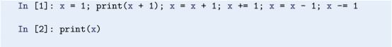
  Then type it in and confirm that your predictions are correct.

• b) Repeat the previous task, but this time without statements number 3 and 4 (counted from left) of the first input line. To confirm your prediction this time, use the command history facility to first bring up the previous command line, which you then edit appropriately before pressing enter.

Remarks

With our statements here, it would clearly have been more readable to write them on separate lines (also making the semi-colon superfluous). Generally, this is also the case, although the possibility of writing several statements on a single line comes in handy from time to time.

Exercise 2.5: Boolean Expression—Even or Odd Number?

Let x be an integer. Use the modulo operator and suggest a boolean expression that can be used to check whether that integer is an even number (or odd, since if not even, the integer is odd). Then check your suggestion interactively, e.g., for x being 1, 2, 3 and 4.

Exercise 2.6: Plotting Array Data

Assume four members of a family with heights 1.60 m, 1.85 m, 1.75 m, and 1.80 m. Next door, there is another family, also with four members. Their heights are 0.50 m, 0.70 m, 1.90 m, and 1.75 m.

• a) Write a program that creates a single plot with all the heights from both families. In your code, use the zeros function from numpy to generate three arrays, two for keeping the heights from each family and one for “numbering” of family members (e.g., as 1, 2, 3 and 4). Let the code overwrite the zeros in the arrays with the heights given, using appropriate assignment statements. Let the heights be presented as two continuous curves in red and blue (solid lines), respectively, when the heights of each family are plotted against family member number. Use also the axis function for the plot, so that the axis with family member numbers run from 0 to 5, while the axis with heights cover 0 to 2.

• b) Suggest a minor modification of your code, so that only data points are plotted. Also, confirm that your suggestion works as planned.

Filename: plot_heights.py.

Exercise 2.7: Switching Values

In an interactive session, use linspace from numpy to generate an array x with the numbers 1.0, 2.0 and 3.0. Then, switch the content of x[0] and x[1], before checking x to see that your switching worked as planned.

Filename: switching_values.py.

Exercise 2.8: Drawing Random Numbers

Write a program that prints four random numbers, from the interval [0, 10], to the screen. To generate the numbers, the program should use the uniform function from the random module of the standard Python library.

Filename: drawing_random_numbers.py.