Boundary Value Problems: Numerical (Approximate) Methods

Abstract

In Chapter 5, we discussed analytic methods of solution for electrostatic problems. The most outstanding feature of these methods was that the solution was exact and in the form of a mathematical relation. On the other hand, only certain classes of problems could be solved. In the case of the method of images, the question was one of finding the correct system of images, a requirement that meant, almost always, that a constant potential surface exists or can be stipulated. If this conducting surface is very complex, the condition of zero potential on the surface may not be as easy to satisfy. Similarly, separation of variable, while certainly valid in general, is often difficult to apply because of the need to satisfy complex boundary conditions. If the boundaries of the problem are not parallel to coordinates, it is next to impossible to find the constants required for solution. Even for the simple planar geometries discussed in Chapter 5, the solution required considerable skill. Furthermore, precious little was said about solution of Poisson’s equation. For another example of the difficulty in analytic solutions, consider Fig. 6.1, which shows a simple parallel plate capacitor. Suppose we need to calculate its capacitance. One method we used before is to assume that the plates are very close to each other, neglect fringing, and use the formula for the parallel plate capacitor. In Fig. 6.1a, the distance between the plates is very small, and the capacitance may be approximated as C = εA/d [F]. Figure 6.1b shows the same two plates, but now the plates are much farther apart, perhaps because our design requires that this capacitor withstand high voltages. Here, we cannot neglect fringing, and, therefore, the use of the formula for parallel plate capacitors is incorrect. How can we solve this problem? It seems that none of the methods of the previous chapters applies here. Yet, this type of problem is quite common. Other examples are the voltage and fields of power lines in the presence of conducting objects (such as transformers, towers, buildings, etc.), field distributions between nonparallel surfaces, and many others. Although, in some cases, assumptions can be made to simplify the problem, this is not always possible and we are faced with the need to solve problems for which analytic methods cannot be used.

Although this may seem a paradox, all exact science is dominated by the idea of approximation

Bertrand Russell, (1872–1970),

philosopher, mathematician, historian

Problems

6.1.1 Finite Differences

• 6.1 One-Dimensional Geometry. A parallel plate capacitor is shown in Figure 6.41. The parallel plates may be viewed as infinite in extent. With d = 1 m and free space between the plates:

  • (a) Calculate the potential distribution everywhere within the capacitor using the finite difference method with four equal divisions.

  • (b) Repeat the solution in (a) with eight equal division.

  • (c) Calculate the potential distribution using direct integration. Show by comparison with (a) and (b) that the division does not matter in this case. Why?

    

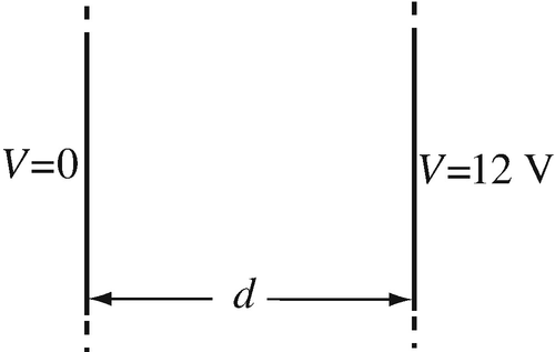
    Figure 6.41

• 6.2 Application: Capacitor with Space Charge Between Plates. The parallel plate capacitor in Figure 6.41 is given. In addition to the data in Problem 6.1, there is also a charge density everywhere inside the material such that ρ/ε = 1 C/F·m², where ρ is the charge density [C/m³] and ε is the permittivity [F/m] of the dielectric between the plates:

  • (a) Find the potential distribution everywhere within the capacitor using four equal divisions.

  • (b) Repeat the solution in (a) with eight equal divisions. Show that the division chosen is important. Which division gives a better result? Compare with the analytical solution.

• 6.3 Capacitor with Space Charge. Consider the parallel plate capacitor in Figure 6.42. A uniform charge density ρ₀ = 10⁻⁶ C/m³ exists everywhere inside the capacitor and both plates are grounded. The permittivity of the material inside the capacitor equals 4ε₀ [F/m]. Assume the plates are very large:

  • (a) Calculate the potential and electric field intensity everywhere inside the capacitor using a one-dimensional finite difference method.

  • (b) Find the analytic solution by direct integration and compare the numerical and analytic solutions.

    

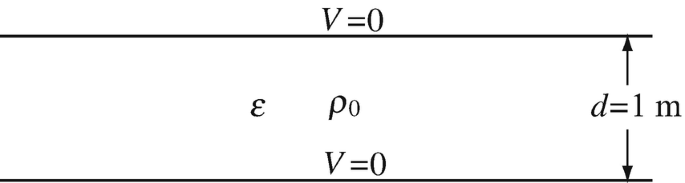
    Figure 6.42

• 6.4 Infinite Channel. Solve for the electric potential in the geometry in Figure 6.43. This is a two-dimensional problem in the form of an infinite channel shown in cross section. The top conducting surface is physically separated from the side plates and is held at a potential 10 V whereas the side and lower boundaries are grounded (held at zero potential). Given: ε = ε₀ [F/m], ρ_v = 0. Use an explicit method of solution.

  

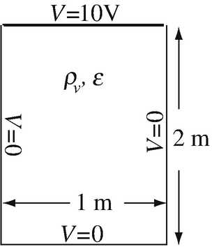
  Figure 6.43

• 6.5 Infinite Channel with Interior Charge. Solve for the electric potential in the geometry given in Figure 6.43. The outer boundaries of the channel are grounded except for the top surface which is at 10 V and a uniformly distributed volume charge distribution exists inside the channel as shown. Given: ρ_v = 10⁻⁶ C/m³, ε = 80ε₀ [F/m].

• 6.6 Infinite Channel with Interior Charge. Solve for the electric potential in the geometry in Figure 6.44. This is a two-dimensional problem similar to that in Problem 6.4, with the outer boundaries grounded and a charge distribution exists inside part of the channel as shown. Given: ρ_v = 10⁻⁶ C/m³, ε₁ = 80ε₀ [F/m].

  

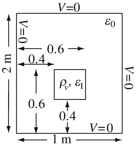
  Figure 6.44

6.1.2 Method of Moments

• 6.7 Application: Capacitance of Small Plates. Two rectangular plates are used as a variable capacitor by rotating one plate about the axis A–A while the other plate is fixed. In the two extremes, the plates are either parallel to each other or flat on a plane as shown in Figures 6.45a and 6.45b. The plates are 50 mm by 20 mm in size. When parallel to each other, they are 2 mm apart, as shown in Figure 6.45b. When on a plane, they are separated 2 mm while the edges remain parallel. Calculate the range of the capacitor’s capacitance in free space.

  

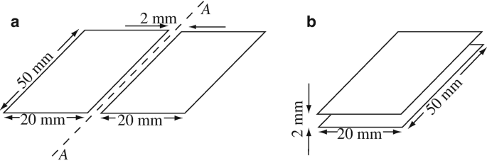
  Figure 6.45

• 6.8 Application: Small Capacitor. A parallel plate capacitor is made from two plates, as shown in Figure 6.46a. The material between the plates is free space:

  • (a) Calculate the capacitance of the capacitor.

  • (b) Now the capacitor is cut in two as shown in Figure 6.46b. Calculate the capacitance of one of the two smaller capacitors thus created. Is the sum of the capacitance of the two halves in Figure 6.46b equal to the capacitance of the whole capacitor in Figure 6.46a? If not, why not?

    

    Figure 6.46

• 6.9 Application: Small Capacitor. Consider Figure 6.46a:

  • (a) Show by a series of calculations with increasing number of subdomains that as the number of subdomains increases, the capacitance of the small capacitor convergences to a constant value. What is this value?

  • (b) Plot the charge density on the upper plate on a line parallel to one of the sides of the plate and that crosses through the center of the plate (or very close to it). Comment on the shape of this plot and its meaning.

• 6.10 Application: Capacitance of a Washer. Calculate the capacitance capacitance of a thin, flat washer of internal radius c = 10 mm and external radius d = 60 mm.

• 6.11 Application: Coupled-Charge Devices (CCD). In a memory array or a CCD (coupled-charge device), capacitive devices are arranged in a two-dimensional array. A 3 × 3 section is shown in Figure 6.47. The purpose of these capacitors is to store charge for a relatively short period of time. Each plate is 2 μm by 2 μm and the separation between two plates is 0.5 μm. As part of the analysis of the device, it is required to calculate the capacitances as follows (assume the plates are in free space):

  • (a) Between each two nearest plates (plates A and B).

  • (b) Between each plate and the plate on the diagonal (plates A and C).

    

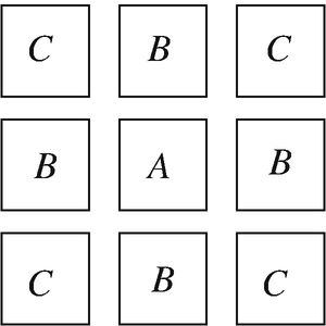
    Figure 6.47

• 6.12 Capacitance of Perpendicular Plates. Two plates with given dimensions form a capacitor as shown in Figure 6.48. The plates are perpendicular to each other. With the dimensions given and assuming the plates are in air (free space):

  • (a) Calculate the capacitance between the plates using the method of moments and hand computation. Use a small, reasonable number of subdomains.

  • (b) If the potential difference between the plates is 1 V, what is the potential and the electric field intensity at point P? Use the charge densities obtained in (a) to calculate the potential at P.

  • (c) Write a program (or use script mom1.m) to calculate a sequence of results, each with increasing number of subdomains until the change in solution is less than 5%. What is the minimum number of subdomains needed if all subdomains must be of the same size?

  

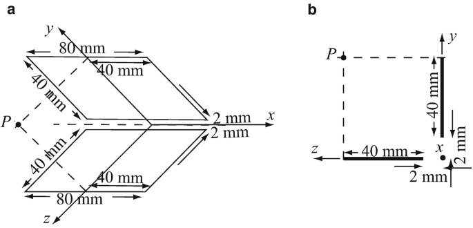
  Figure 6.48

• 6.13 Capacitance Between Two Unequal Plates. The two plates in Figure 6.49 are given. Calculate the capacitance between the plates assuming they are in free space.

  • (a) Use hand computation with 4 equal elements on each of the plates.

  • (b) Use script mom1.m and a sequence of divisions of the plates to obtain a more accurate solution. Use the same number of divisions on each plate and increase the number of divisions until the capacitance does not change by more than 1%. What is the capacitance and how many divisions on each plate are needed?

    

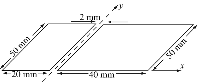
    Figure 6.49

6.1.3 Finite Elements

• 6.14 One-Dimensional Finite Elements. A one-dimensional element may be defined in a manner similar to that in Section 6.5.1.1 by assuming a section of a line of finite length, two points at its ends with coordinates (x₁) and (x₂), and unknown values ϕ₁ and ϕ₂ as shown in Figure 6.50:

  • (a) For this element, calculate the shape functions necessary to define the element by assuming a linear variation inside the element of the form ϕ(x) = a + bx.

  • (b) With the shape functions in (a), find an expression for the function ϕ(x) inside the element in terms of the shape functions.

  • (c) Show that the magnitude of N₁ [shape function at node (1)] is 1 at node (1) and zero at node (2).

  • (d) Show that the magnitude of N₂ [shape function at node (2)] is 1 at node (2) and zero at node (1).

  • (e) Show that the sum of the shape functions at any point x₁ ≤ x ≤ x₂ equals 1.

    

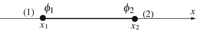
    Figure 6.50

• 6.15 Application: Field and Potential in Parallel Plate Capacitor. Consider the parallel plate capacitor with a dielectric between the plates shown in Figure 6.51. The dielectric has relative permittivity of 6 and a volume charge distribution as shown: Assume plates are very large:

  • (a) Set up a finite element solution and solve for the potential, using the shape functions in Problem 6.14. Use hand computation and as many elements as necessary.

  • (b) From the potential distribution, calculate the electric field intensity in the capacitor. Sketch the solutions.

  • (c) Find the analytic solution for potential by direct integration and compare with the results in (a).

    

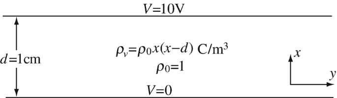
    Figure 6.51

• 6.16 Application: Field and Potential in Parallel Plate Capacitor. Consider Figure 6.52. Using the triangular shape functions defined in Section 6.5.1 and the implementation in Section 6.5.2:

  • (a) Calculate the potential distribution inside the capacitor. Assume plates are very large.

  • (b) From the potential distribution, calculate the electric field intensity in the capacitor. Sketch the solutions.

  • (c) Find the analytic solution and compare with (a) and (b).

    

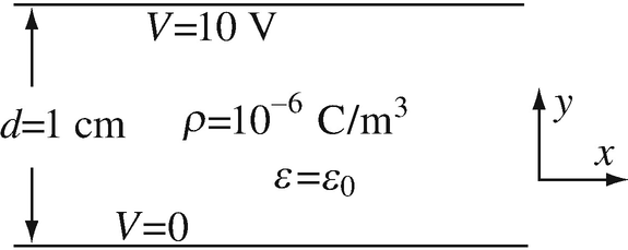
    Figure 6.52

• 6.17 Quadrilateral Finite Elements. Figure 6.53 shows a two-dimensional, four-node element (quadrilateral element). Assume an approximation of the form ϕ(x,y) = a + bx + cy + dxy:

  • (a) Define the shape functions and their derivatives for a particular element with nodes at P₁(0,0), P₂(1,0), P₃(1,1), and P₄(0,1).

  • (b) Define the shape functions and their derivatives for the general element in Figure 6.53.

  • (c) Discuss the method and comment on its extension to more complex finite elements.

    

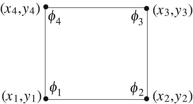
    Figure 6.53

• 6.18 Application: Breakdown in Microcircuits. One of the challenges of microcircuits is the need for an ever-decreasing size of components. This means that components must be closer to each other and, therefore, the danger of breakdown between components and, in particular, between lines leading to them. To see the difficulty involved, consider the following: In a microcircuit, the smallest width conducting lines are 0.5 μm. Two such lines run side by side as shown in Figure 6.54. Assume the material below the lines is silicon with a relative permittivity of 12, and above and between the lines, it is free space. Breakdown in air occurs at 3 × 10⁶ V/m and in silicon at 3 × 10⁷ V/m. Assume the silicon layer is very thick:

  • (a) If the minimum distance between lines is d = 0.5 μm, what is the maximum potential difference allowable between the two lines? This is usually taken as the maximum source voltage for the circuit.

  • (b) If the circuit must operate on a maximum potential difference of 5 V, what is the minimum distance d [μm] allowed between the lines?

    

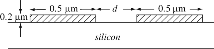
    Figure 6.54

• 6.19 Application: Breakdown in Printed Circuits. The width of two strips on opposite sides of a printed circuit board is 1 mm and their thickness is 0.1 mm as shown in Figure 6.55a. The material is 0.5 mm thick, made of fiberglass with relative permittivity of 3.5. Breakdown voltage in fiberglass occurs at 30 kV/mm:

  • (a) What is the maximum potential difference allowable between the two strips?

  • (b) Suppose the printed circuit board has a flaw so that the material between the strips is missing, as shown in Figure 6.55b. What is now the maximum electric potential allowable?

    

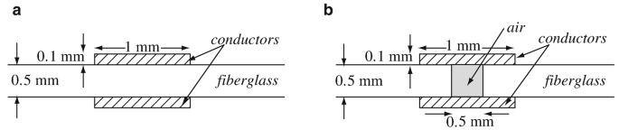
    Figure 6.55

• 6.20 Application: Potential in Three-Phase Underground Cable. A three-phase power line operates at 240 V peak and is enclosed in a conducting shield which is at zero potential. The space between conductors and shield is filled with a material with relative permittivity 2.0:

  • (a) Assume the lines are very thin (Figure 6.56a) and calculate the potential distribution everywhere in the cable. Plot constant potential lines. The conditions are r = 0.05 m, d = 0.01 m, V₁ = 240 V, V₂ = 240cos(120°) [V], and V₃ = 240cos(240°) [V].

  • (b) The actual lines are each 10 mm in diameter (Figure 6.56b). Calculate the potential distribution everywhere in the cable. The conditions are r = 0.05 m, d = 0.01 m, V₁ = 240 V, V₂ = 240cos(120°) [V], and V₃ = 240cos(240°) [V]. Hint: The conductor surfaces become boundary conditions with known potentials. No need to discretize the interior of the conductors.

    

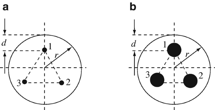
    Figure 6.56