Boundary Value Problems: Analytic Methods of Solution

Abstract

The relations and methods introduced in Chaps. 3 and 4 dealt primarily with point and distributed charges and the electric fields they produce. If the charges were known, the electric field and potential could be determined. However, many practical situations exist in which the charges are either unknown or are distributed in a complex fashion. The use of the simple formulas for the calculation of fields in these geometries is not always possible. In still other geometries, we have no knowledge of charges but only of fields and potentials. For example, in an overhead transmission line, we may know the potential but not the charge on the line. How can we then calculate the electric field intensity everywhere in space? Similarly, when designing an electric instrument, such as an electrostatic filter, the engineer is not going to calculate “how much charge must be present on the electrode.” This information, while important in itself, is not normally a design parameter simply because we do not usually use “charge supply sources” and we are ill equipped to measure charge or charge density. The more common problem in design would be to calculate the required potential on the electrodes of the device to produce the needed effect. This information is important because with it, the power supply required can be designed. Although the principles in Chaps. 3 and 4 and the formulas developed for calculation of fields, potentials, and energy are applicable to these types of problems as well, the difficulty is in applying them.

If there is no other use discover’d of Electricity, this, however, is something considerable, that it may help to make a vain man humble.

—Benjamin Franklin (1706–1790)

statesman, scientist, inventor

Problems

5.1.1 Laplace’s and Poisson’s Equations

• 5.1 Solution to Laplace’s Equation. The solution of Laplace’s equation is known to be V = f (x)g(y) = fg, where f and g are scalar functions, f is a linear function of x alone, and g is a linear function of y alone. Which of the following are also solutions to Laplace’s equation?

  • (a) V = 2fg.

  • (b) V = fg + x + yg.

  • (c) V = 2f + cg, where c is a constant.

  • (d) V = f²g.

• 5.2 Solution to Laplace’s Equation. The potential produced by a point charge Q [C] at a distance R [m] in free space is given as V(R) = Q/4πε₀R [V].

  • (a) Show that this potential satisfies Laplace’s Equation at any R except R = 0.

  • (b) What happens at R = 0?

5.1.2 Direct Integration

• 5.3 Application: Potential Distribution in a Capacitor. A parallel plate capacitor with distance between plates of 2 mm contains between its plates a dielectric with permittivity ε = 4ε₀ [F/m]. The potential difference between the plates is 5 V. Suppose the plate at x = 0 is at zero potential, the plate at x = 0.002 m is at 5 V. Find V(x) everywhere assuming there are no edge effects.

• 5.4 Application: Uniform Space Charge Density in a Capacitor. The parallel plate capacitor in Figure 5.33 contains a dielectric with permittivity ε₀ [F/m] and a constant charge density ρ_v = ρ₀ [C/m³] distributed uniformly throughout the dielectric. Assume the plates are infinite and calculate the potential everywhere between the plates.

• 5.5 Nonuniform Space Charge in a Capacitor. A parallel plate capacitor with plates separated a distance d = 2 mm is connected to a 100 V source as in Figure 5.33. The space between the plates is air, but there is also a charge distribution between the plates given as ρ_v = 10^–6x(x – d) [C/m³] where x is the distance from the zero voltage plate. Assume the plates are large and calculate the potential everywhere between the plates.

Figure 5.33

• 5.6 Application: Potential and Field in Coaxial Cables. Coaxial cables used for cable TV also distribute power to amplifiers and other devices on the lines. Suppose a standard coaxial cable with an inner conductor made of a solid wire 0.5 mm in diameter and an outer, thin conducting shell 8 mm in diameter is used. A DC voltage of 64 V is connected with the positive pole connected to the inner conductor. Calculate:

  • (a) The potential distribution everywhere in the coaxial cable.

  • (b) The electric field intensity everywhere in the coaxial cable.

  • (c) Plot the potential and the electric field intensity as a function of distance from the center of the cable.

• 5.7 Potential Due to Large Planes. Two conducting planes at 45° are connected to potentials as shown in Figure 5.34. The two planes do not meet at the origin (a small gap exists between them). If a potential V₀ is given on the horizontal plane, with reference to the inclined plane, calculate:

  • (a) The potential everywhere between the plates in the 1st octant.

  • (b) The potential everywhere in the rest of the space.

    Hint: use cylindrical coordinates

Figure 5.34

• 5.8 Application: Potential and Field in Spherical Capacitor. A spherical capacitor is made of two concentric shells. The inner shell is 10 mm in diameter. The outer shell is 10.1 mm in diameter. A potential V₀ = 50 V is connected across the two shells so that the positive pole of the battery is connected to the inner shell. The space between the shells is filled with a dielectric with a relative permittivity of 2.25. Calculate:

  • (a) The potential everywhere between the shells. Does the potential depend on permittivity? Explain.

  • (b) The electric field intensity everywhere between the shells.

  • (c) Plot the potential and electric field intensity as a function of distance from the inner shell.

• 5.9 Spherical Charge Distribution The potential inside a spherical charge distribution centered at the origin is given as V(R) = cR² [V] where c is a constant. The permittivity in the charge distribution is ε [F/m]. Calculate the volume charge density that produces this potential.

5.1.3 Method of Images: Point and Line Charges in Planar Configurations

• 5.10 Point Charge Above a Conducting Plane. A 5 nC point charge lies 2 m above a conducting plane. Find the surface charge density:

  • (a) Directly below the point charge, on the conducting plane.

  • (b) 1 m from the point in (a) (sideway).

• 5.11 Point Charges Above a Conducting Plane. Two point charges are located above a conducting plane as shown in Figure 5.35. Calculate the electric field intensity:

  • (a) In the space above the plane.

  • (b) At the surface of the conductor.

Figure 5.35

• 5.12 Charged Line Above a Conducting Plane. A very long charged line is located above a perfectly conducting plane in free space as shown in Figure 5.36. The charge density on the line is ρ_l [C/m]:

  • (a) Find the surface charge density on the conducting plane.

  • (b) Show that the total charge per unit depth of the conducting surface equals –ρ_l [C/m].

Figure 5.36

• 5.13 Charged Line and Multiple Conducting Planes. An infinitely long line charged with a line charge density ρ_l [C/m] is located at a distance d [m] from a very large conductor, as in Figure 5.37:

  • (a) Calculate the electric field intensity and the potential on the dotted line shown.

  • (b) A second conducting surface is now placed to fill the space to the right of the dotted line. What are now the electric field intensity and potential on this line? Compare with the results in (a).

    

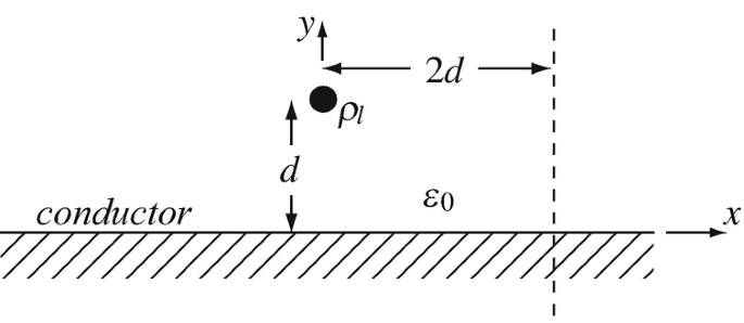
    Figure 5.37

5.1.4 Method of Images: Multiple Planes

• 5.14 Point Charge Between Conducting Planes. A point charge Q [C] is located midway between two conducting plates in free space. The plates intersect at 45° to each other:

  • (a) Show that the electric field intensity is perpendicular to the plates everywhere.

  • (b) Calculate the charge density induced on the plates if the radial distance from the intersection of the plates to the point charge is d [m].

• 5.15 Point Charge Between Intersecting Conducting Planes. Two conducting planes intersect at 30°, as in Figure 5.38. Both surfaces are at zero potential. A point charge q [C] is placed midway between the two planes at point A, as shown.

• (a) Draw the system of image charges and calculate the electric field intensity everywhere between the planes, assuming free space.

• (b) Show by means of a drawing what happens if the charge is moved from the center toward the upper plane so that it is at a distance b [m] from the upper plane and a distance c [m] from the lower plane while the radial distance is maintained (point B).

• (c) Show by means of a drawing what happens if the angle between the planes is not an integer divisor of 180°. Use an angle of 75° as an example.

  

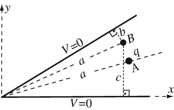
  Figure 5.38

• 5.16 Point Charge Between Parallel Conducting Planes. A point charge is placed between two infinite planes in free space, as in Figure 5.39:

  • (a) Show the location and magnitude of the first few image charges.

  • (b) Place a system of coordinates so that the upper plate is at x = 0 and the point charge is at (x = 3d/4, y = 0), and calculate the potential at the middle point between the plates (x = d/2, y = 0) using the first six image charges (plus the original point charge).

Figure 5.39

• 5.17 Point Charge Between Parallel Conducting Planes. A point charge is placed between two infinite planes in free space, as in Figure 5.39:

  • (a) Place a system of coordinates so that the upper plate is at x = 0 and the point charge is at (3d/4,0). Find an expression for the potential at any point between the two plates as a sum on N image charges.

  • (b) Optional: Write a computer program or a script that will evaluate the sum in (a) for N = 7, N = 100, N = 1,000, and N = 100,000, at x = 0.05 m, y = 2.0 m using q = 1 × 10^–12 C, d = 0.5 m. Compare the results and provide an indication of how many image charges are necessary for a maximum relative error of 1%.

• 5.18 Point Charge Between Parallel Conducting Planes. Consider a point charge embedded in a dielectric material as shown in Figure 5.40. The dielectric, of permittivity ε₁ [F/m], is bound by two parallel plates, each held at a constant potential V₀ [V]:

  • (a) Can you use the method of images to find the field inside the dielectric. How?

  • (b) If so, find the first four image charges and their location and calculate the potential at any point between the plates. Place a system of coordinates so that the upper plate is at x = 0 and the point charge is at (d₂,0).

Figure 5.40

• 5.19 Point Charge in Infinite Closed Channel. Figure 5.41 shows a hollow cavity in a conducting medium. The cavity is infinite in the dimension perpendicular to the plane shown:

  • (a) Show the location of the image charges necessary to calculate the electric field intensity inside the cavity.

  • (b) Use the nearest four images and the charge q [C] to calculate an approximate value for the electric field intensity at the center of the box, in the plane shown. Place a system of coordinates so that the lower left corner of the cavity is at (0,0).

Figure 5.41

• 5.20 Point Charge in Infinite Closed Channel. The cavity in Figure 5.41 is given. The cavity is infinite in the dimension perpendicular to the plane shown:

  • (a) Show the image charges locations.

  • (b) Place a system of coordinates so that the lower left corner of the cavity is at (0,0) and find a general expression for the potential at a general point within the cavity.

  • (c) Evaluate the expression in (b) using the closest eight image charges (plus the original charge) at the center of the cavity.

  • (d) Optional: Write a computer program or a script that will evaluate the sum in (b) at x = 1.0 m, y = 2.0 m, for the closest N = 9, N = 100, N = 1,000, and N = 100,000 charges. Use q = 1 × 10^–9 C, a = 5m, b = 10 m, c = 2.5 m, d = 2.5 m. Compare the results and provide an indication on how many image charges are necessary for a maximum incremental error of 1%.

5.1.5 Method of Images in Curved Geometries

• 5.21 Application: Cable in a Tunnel. A cable runs through a mine shaft suspended from the ceiling as shown in Figure 5.42. The cable is thin and carries a charge of 10 nC per meter. The shaft is 10 m in diameter. Calculate the electric field intensity at the center of the shaft (magnitude and direction). Assume soil is conducting, and the air in the shaft has permittivity of free space.

Figure 5.42

• 5.22 Application: Two Charged Wires Next to a Conducting Cylinder. Two wires, one charged with a positive line charge density and one with a negative line charge density, run parallel to a thick conducting pipe in free space as shown in Figure 5.43. Calculate the electric field intensity everywhere.

Figure 5.43

• 5.23 Point Charge in a Conducting Shell. A point charge +q [C] is located inside a very thin conducting spherical shell halfway between the center and the shell shown in Figure 5.44. Assume the conducting shell is at zero potential:

  • (a) Calculate the electric field intensity at the center of the sphere assuming free space inside the shell.

  • (b) What is the field outside the sphere?

  • (c) Plot the electric field intensity inside the sphere by plotting the field lines (approximate plot is sufficient).

Figure 5.44

• 5.24 Point Charge Outside a Conducting Sphere. For the conducting sphere and point charge shown in Figure 5.45, find:

  • (a) The image charge (magnitude and location).

  • (b) The electric field intensity on the surface of the sphere.

  • (c) The induced charge density on the surface of the sphere.

  • (d) Sketch the electric field intensity outside the sphere.

Figure 5.45

• 5.25 Point Charge Inside Hollow, Charged Conducting Sphere. Solve Problem 5.23 if the shell is at a constant potential V₀ [V]. Sketch the electric field intensity outside the shell.

• 5.26 Point Charge Outside Charged Conducting Sphere. Solve Problem 5.24 if the shell has a positive surface charge density ρ_s [C/m²]. The potential on the shell need not be zero.

• 5.27 Two Point Charges Outside Grounded Conducting Sphere. A grounded (zero potential) conducting spherical shell of radius a [m] and two point charges are located in free space as shown in Figure 5.46:

  • (a) Calculate the electric field intensity at a general point outside the sphere in thgw y–z plane if c > a and d > a.

  • (b) What is the electric field intensity outside the sphere if c, d → ∞? Explain.

  • (c) What is the electric field intensity at a general point inside the sphere if c < a and d < a.

  • (d) What is the electric field intensity at a general point inside the sphere if c, d → 0? Explain.

Figure 5.46

5.1.6 Separation of Variables in Planar Geometries

• 5.28 Potential in Infinite Channel. The geometry in Figure 5.47 is made of a semi-infinite channel bounded by the planes x = 0, x = ∞, y = 0, y = b [m]. Three sides are held at zero potential and the fourth is isolated from the others (between y = 0 and y = b) and held at potential V₀ [V]. Find the potential within the channel.

Figure 5.47

• 5.29 Potential in Infinite Channel. The infinite channel shown in Figure 5.48 is made of three conducting walls connected to a zero potential, and a fourth is an isolated wall (top cover) connected to a potential V_u. The cover and sides are close to each other but are not touching. The material in the channel is free space:

  • (a) Calculate the potential everywhere in the channel if V_u = 10 V (DC).

  • (b) Plot the potential as a sequence of constant potential lines inside the box.

Figure 5.48

• 5.30 Potential in Infinite Channel. Figure 5.48 shows the cross section through an infinitely long channel. Three sides are connected to ground potential, and the top is insulated from the rest of the structure and connected to a potential V_u as shown. The channel is filled with a material with permittivity ε [F/m]. Calculate the potential everywhere inside the cross section if V_u = 10sin(πx/a) [V].

• 5.31 Potential in Infinite Channel. A two-dimensional geometry consists of four infinitely long plates, shown in cross section in Figure 5.49. For the given plate potentials, calculate the electric potential at a general point between the plates.

Figure 5.49

• 5.32 Potential in a Box with Conducting Walls. A three-dimensional cubic box, with dimensions a × a × a [m³], is grounded on four sides. The two sides at z = a [m] and at x = a [m] are connected to a constant potential as shown in Figure 5.50. Calculate the potential everywhere inside the box.

Figure 5.50

5.1.7 Separation of Variables in Cylindrical Geometries

• 5.33 Application: Electrostatic Precipitator. An electrostatic precipitator is made by lining the interior of a smokestack with two half-shells as shown in cross section in Figure 5.51. Assume the stack is very long and a potential difference of 100 kV is connected as shown. Ground is at zero potential so that the left half-shell is at – 50 kV and the right half-shell at +50 kV. Calculate:

  • (a) The potential inside and outside the stack.

  • (b) The electric field intensity inside and outside the stack.

Figure 5.51

• 5.34 Application: Electrostatic Precipitator. The designers of the precipitator in Problem 5.34 found that they cannot make two half-shells as needed, but they can make the precipitator of four quarter-shells and connect them as shown in Figure 5.52. Calculate:

  • (a) The potential inside and outside the stack.

  • (b) The electric field intensity inside and outside the stack.

Figure 5.52