Gauss’s Law and the Electric Potential

Abstract

The fundamentals of electrostatics were given in Chapter 3 as the definition of force through Coulomb’s law and of the electric field intensity. In this chapter, we address two issues: one is to formalize some of the results obtained in the previous chapter and the second is to expand on the ideas of electric field intensity, electric flux density, and the relation between the electric field and material properties.

I have had my results for a long time but I do not yet know how I am to arrive at them.

—Johann Carl Friedrich Gauss (1777–1855)

(A. Arber, The Mind and the Eye, 1954)

Problems

4.1.1 Postulates

• 4.1 Charge Density Required to Produce a Field. A layer of charge fills the space between x = –a [m] and x = +a [m]. The layer is charged with a nonuniform volume charge density ρ(x) [C/m³]. The electric field intensity everywhere inside the charge distribution is given by $\mathbf{E}(x)=\hat{\mathbf{x}}K{x}^3$ [N/C], where K is a given constant. Assume the layer is in free space:

  • (a) Calculate the volume charge density ρ(x).

  • (b) What can you say about the charge density for x > 0 and for x < 0?

  • (c) How does the charge density vary in the y and z directions?

• 4.2 Charge Density Required to Produce a Given Field. A volume charge density is distributed throughout the free space. The electric field intensity at a distance R from the origin is given as $\mathbf{E}=\hat{\mathbf{R}}k{R}^2\kern0.5em \left[\mathrm{V}/\mathrm{m}\right]$ in free space, where k is a constant.

  • (a) Calculate the volume charge density that produces this field.

  • (b) Show that the given field is a valid electric field.

• 4.3 Electrostatic Fields. Which of the following vector fields are electrostatic fields? Justify your answer.

  • (a) $\mathbf{A}=\hat{\mathbf{x}} yz+\hat{\mathbf{y}}2x$.

  • (b) $\mathbf{A}=\hat{\mathbf{R}}{bR}^3+\hat{\boldsymbol{\uptheta}}c$ where b and c are constants.

  • (c) $\mathbf{A}=\hat{\boldsymbol{\upphi}}r$.

  • (d) $\mathbf{A}=\hat{\mathbf{R}}\left({10}^{-8}/{R}^3\right)\cos \theta +\hat{\boldsymbol{\uptheta}}\left({10}^{-8}/2{R}^3\right)\sin \theta$.

4.1.2 Gauss’s Law: Calculation of Electric Field Intensity from Charge Distributions

• 4.4 Electric Field Due to Spherical Distribution of Charge. A spherical region 0 ≤ R ≤ 2 mm contains a uniform volume charge density of 100 nC/m³, whereas another region, 4 mm ≤ R ≤ 6 mm, contains a uniform charge density of –200 nC/m³. If the charge density is zero elsewhere, find the electric field intensity for (assume ε = ε₀):

  • (a) R ≤ 2 mm.

  • (b) 2 mm ≤ R ≤ 4 mm.

  • (c) 4 mm ≤ R ≤ 6 mm.

  • (d) R ≥ 6 mm.

• 4.5 Application of Superposition. A dielectric sphere of radius 3a [m] has two spherical hollows, one of radius a [m] and one of radius 2a [m] as shown in Figure 4.56. A total charge Q [C] is distributed uniformly throughout the solid part of the volume. Assume the sphere is made of a material with permittivity ε₀ [F/m]. Calculate the electric field intensity at point P.

  

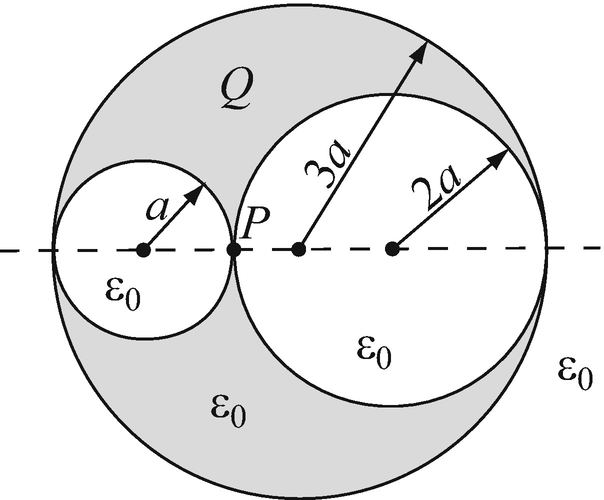
  Figure 4.56

• 4.6 Fields of Point and Distributed Charges. A point charge Q [C] is placed at the origin of the system of coordinates. A concentric spherical surface with radius R = a [m] with a uniform surface charge density ρ_s [C/m²] in free space surrounds the point charge:

  • (a) Find E everywhere.

  • (b) Find the required surface charge density ρ_s in terms of Q such that the electric field intensity is zero for R > a.

• 4.7 Electric Field Due to Planar Charge Density. An infinite plane, charged with a uniform surface charge density ρ₀ [C/m²], is immersed in a dielectric of permittivity ε [F/m]. Calculate the electric field intensity:

  • (a) Everywhere.

  • (b) Everywhere if the dielectric is removed.

• 4.8 Superposition of Fields of Planar Charges. A charge distributiondistribution consists of two parallel, infinite plates, charged with equal but opposite surface charge densities ρ_s [C/m²] separated a distance 2a [m] apart, two additional infinite plates separated a distance 2b [m] apart and charged in a similar fashion, and a uniformly distributed volume charge density ρ_v [C/m³] between the two inner plates (Figure 4.57). Calculate the electric field intensity everywhere. Assume permittivity of free space everywhere.

  

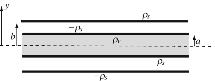
  Figure 4.57

• 4.9 Superposition of Fields of Planar Charges. Two very large (infinite) charged planes intersect at 90° as shown in Figure 4.58. The four quadrants are each made of a different material as shown. The planes are charged uniformly with positive surface charge density +ρ_s [C/m²]:

  • (a) Find the electric field intensity everywhere.

  • (b) A positive point charge +q [C] is placed at a general point in space P(x,y), but not on the planes. Calculate the force (magnitude and direction) on this charge.

  • (c) Assuming ε₃ > ε₂ > ε₁ > ε₀, where is the force largest?

    

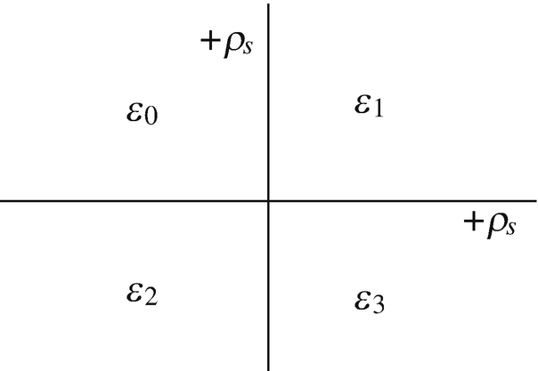
    Figure 4.58

• 4.10 Electric Field Due to a Layer of Charge. A volume charge density is distributed inside an infinite section of the space as shown in Figure 4.59. The distribution is uniform in the y and z directions. The volume charge density depends on x as ρ_v = ρ₀|x| [C/m³]. Calculate the electric field intensity everywhere.

  

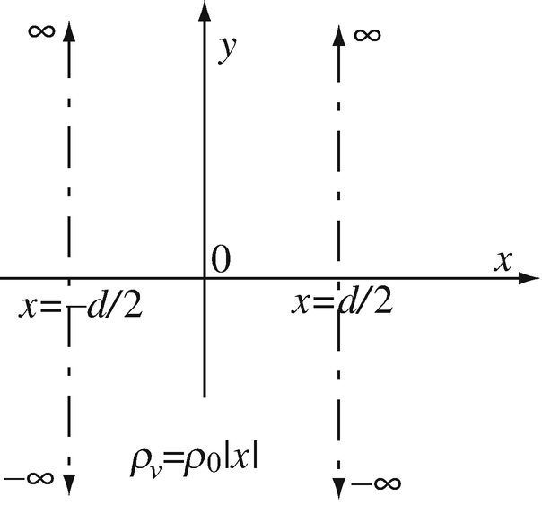
  Figure 4.59

• 4.11 Superposition of Fields Due to Line and Surface Charge Densities. Given a very large sheet with uniform surface charge density ρ_s [C/m²] located at z = z₀ and a long line with uniform line charge density ρ_l [C/m] placed at z = 0, on the x axis in free space:

  • (a) Find the electric field intensity everywhere.

  • (b) Find the electric flux density at point (0,0,1).

  • (c) Find the electric field intensity if the whole geometry is immersed in oil (ε = 4ε₀).

• 4.12 Application: Electric Field Intensity in a Coaxial Line. Two very long cylindrical shells are arranged as shown in Figure 4.60. The shells are uniformly charged with equal and opposite charge densities. The space between the two shells is filled with a dielectric with permittivity ε [F/m]:

  • (a) Find the electric field intensity everywhere.

  • (b) Sketch the electric field intensity everywhere.

  • (c) A line of charge is now introduced on the center axis to produce a zero field outside the outer shell. Calculate the required line charge density.

    

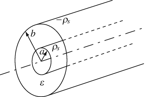
    Figure 4.60

• 4.13 Application: Electric Field intensity in a Two-Conductor Cable. Two parallel cylinders, each 10 mm in radius, are placed in free space and each contains a uniformly distributed charge density of 0.5 μC per meter length. The axes of the cylinders are separated by 4 m. For orientation purposes, place the two conductors on the x–z plane with their axes along the z direction, with the z-axis midway between the conductors and the y axis pointing up. What is the magnitude of the electric field intensity:

  • (a) At a point P₁ midway between the two cylinders?

  • (b) At a point P₂ midway between the two cylinders and two meters below them?

4.1.3 Gauss’s Law: Calculation of Equivalent Charge from the Electric Field Intensity

• 4.14 Charge Distribution Required to Produce a Field. A flat dielectric with permittivity ε [F/m] and thickness d [m] is charged with an unknown volume charge density (Figure 4.61). The dielectric may be assumed to be very large (essentially an infinite slab). The electric field intensity is known inside the dielectric and is given as

  $$ \mathbf{E}=\hat{\mathbf{y}}\frac{y^2}{2}\kern1.5em \left[\frac{\mathrm{N}}{\mathrm{C}}\right]\kern1.5em \mathrm{for}\kern1em \frac{d}{2}>y>0,\kern2em \mathbf{E}=-\hat{\mathbf{y}}\frac{y^2}{2}\kern1.5em \left[\frac{\mathrm{N}}{\mathrm{C}}\right]\kern1.5em \mathrm{for}\kern1em -\frac{d}{2}<y<0 $$

  • (a) What is the volume charge density inside the dielectric?

  • (b) What is the electric field intensity outside the dielectric?

    

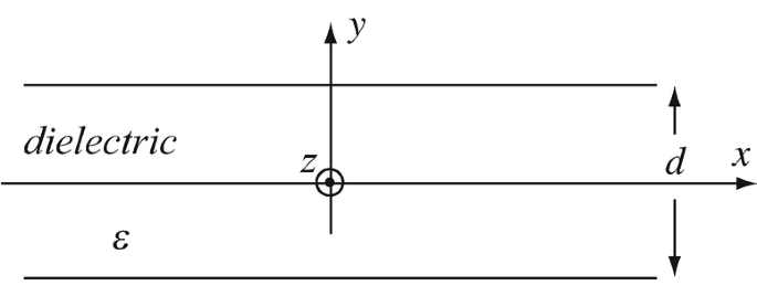
    Figure 4.61

• 4.15 Volume Charge Density Needed to Produce a Field. The electric field intensity is given inside a sphere of radius R ≤ b [m] as $\mathbf{E}=\hat{\mathbf{R}}4{R}^2\ \left[\mathrm{N}/\mathrm{C}\right]$. The sphere has permittivity ε [F/m]. Find:

  • (a) The volume charge density ρ_v at R = b/4 [m].

  • (b) The total electric flux leaving the spherical surface of radius R = b/2 [m].

• 4.16 Maximum Allowable Charge Density on Power Lines. A DC power transmission line is made of two conductors, each 20 mm in diameter and separated a distance 6 m apart. The maximum electric field intensity allowed anywhere in space is 3 × 10⁶ N/C. If one line is positively charged and one is negatively charged, calculate:

  • (a) The maximum surface charge density allowable on the conductors.

  • (b) Suppose the conductors are covered with a 3 mm thick rubber insulation which has a relative permittivity of 3.0. The maximum electric field intensity allowed in rubber is 2.5 × 10⁷ N/C. What is now the maximum surface charge density allowable on the conductors?

4.1.4 Potential: Point and Distributed Charges

• 4.17 Potential Due to a System of Point Charges. Eight equal charges q = 3 nC are placed at the vertices of a cube in a vacuum. Place the cube in a Cartesian system of coordinates so that the faces are parallel to the x–y, x–z, and y–z planes, with one vertex at the origin. The cube is in the positive octant of the system of coordinates. The side of the cube is a = 0.5 m. Find:

  • (a) The potential and the electric field intensity at the center of the cube.

  • (b) The potential and electric field intensity at the center of the face parallel to the x–y plane (at x = a/2, y = a/2, z = a).

• 4.18 Potential Due to Point Charge and Spherical Charge Distribution. A point charge Q [C] is surrounded by a uniform spherical charge distribution of radius a [m], having a uniform volume charge density ρ_v [C/m³]:

  • (a) Calculate the potential everywhere.

  • (b) Plot the potential with respect to position.

• 4.19 Application: Potential and Field Between Charged Plates. The two plates in Figure 4.62 are very large (infinite). The dielectric between the plates is air:

  • (a) Calculate the electric field intensity between and outside the plates.

  • (b) If the potential on the left plate is zero, calculate and plot the potential everywhere.

  • (c) Assume that the potential difference between the plates is increased by V₀. This potential is connected with its positive side to the right plate with the zero potential reference kept as in (b). How does this affect the potential outside and between the plates?

    

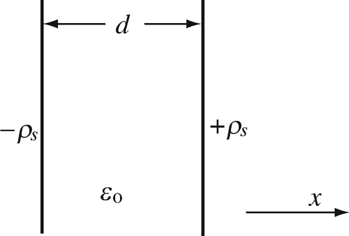
    Figure 4.62

• 4.20 Application: Charge Density in Coaxial Cable Connected to a Battery. A very long, solid cylindrical conductorconductor of radius b [m] is placed at the center of an equally long, thin, cylindrical shell of radius a [m] as shown in Figure 4.63 to form a coaxial line and a voltage source is connected as shown. Calculate:

  • (a) Charge density per unit area on the central conductor.

  • (b) Charge density per unit area on the outer shell.

    

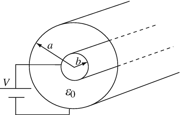
    Figure 4.63

• 4.21 Application: Potential Due to a Charged Disk. A thin disk of radius a [m] carries a uniform surface charge density ρ₀ [C/m²]. Find the potential at a distance d [m], on the axis of the disk (directly above its center) in free space.

• 4.22 Field and Potential Due to Charged Dielectric. Two very large, conducting, parallel plates separated a distance 2a [m] contain a uniform volume charge density ρ_v [C/m³] between them. The plates are very thin and are both at zero potential. Permittivity between the plates is ε [F/m], outside the plates ε₀ [F/m]. Calculate:

  • (a) The electric field intensity everywhere between and outside the plates. Sketch.

  • (b) The potential everywhere between the two plates and outside the plates. Sketch.

4.1.5 Electric Field from Potential

• 4.23 The Potential and Field of a System of Point Charges 2N + 1 point charges are distributed on the x-axis as shown in Figure 4.64. The distance between each two point charges is a [m] and the charges are in free space. Calculate:

  • (a) The potential at a general point P(x,y).

  • (b) The electric field intensity at P(x,y).

    

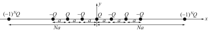
    Figure 4.64

• 4.24 Charge Density and Electric Field Intensity Due to Potential. The electric potential inside a dielectric sphere of radius b [m] and permittivity ε [F/m] is given as V = aR² [V] where a is a constant. The sphere is located in free space. Find:

  • (a) The volume charge density ρ_v inside the dielectric sphere.

  • (b) The electric field intensity E, inside and outside the sphere.

• 4.25 Electric Field Intensity Due to Potential. A potential is given at a general point (x,y,z) in free space as V(x,y,z) = 0.5 [1/(x − 2) + 1/(y − 1) − 2/(z + 2)] [V].

  • (a) Calculate the electric field intensity at any point in space.

  • (b) Show that the result in (a) is a valid electric field intensity.

  • (c) Calculate the volume charge density that produces this field.

• 4.26 The Quadrupole. The potential of a system of point charges is known at a general point (R,θ,ϕ) at a large distance from the charges as

  $$ V\left(R,\theta \right)=C\frac{3\cos^2\theta -1}{R^3}\kern1.5em \left[\mathrm{V}\right] $$

  where R is the distance from the origin, θ the angle between the vector R and the reference z axis and C is a constant.

  • (a) Calculate the electric field intensity at that point.

  • (b) Explain why it is not possible to calculate the point charges that produced this field.

4.1.6 Conductors in the Electric Field

• 4.27 Conductor in a Uniform Electric Field. Two infinite plates are separated a distance 2b [m] in free space. A conducting slab of thickness 2c [m] (c < b) is inserted between the plates as shown in Figure 4.65. The plates are connected to a potential V [V] with the lower plate at zero (reference) potential:

  • (a) Calculate the potential everywhere between the two plates before inserting the conductor.

  • (b) Calculate the potential everywhere after inserting the conductor.

  • (c) Does the vertical position of the conductor between the plates affect the electric field intensity? Explain.

    

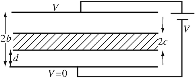
    Figure 4.65

• 4.28 Potential in a Conductor. A point charge Q [C] is placed at the center of a conducting sphere of radius R [m], in a small hollow cavity so that it does not touch the conductor. Calculate the potential at a point r = R/2 [m].

• 4.29 Layered Structures. The device in Figure 4.66 is made as follows: A spherical conductor of radius a [m] is surrounded by a dielectric shell of outer radius b [m] and permittivity ε₁ [F/m]. This shell is surrounded by another spherical shell of outer radius c [m] and permittivity ε₂ [F/m]. On top of this, there is a conducting shell with outer radius d [m]. A potential V₀ [V] is connected between the outer and inner conductors as shown in Figure 4.66. Calculate the charge density on the inner and outer conductors. Where is this charge density distributed?

  

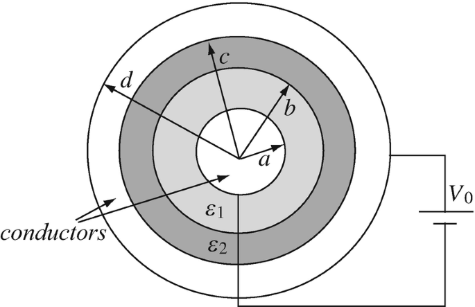
  Figure 4.66

• 4.30 Electric Field and Potential in Spherical Shells and Conductors. Two geometries are given in Figures 4.67a and 4.67b. In Figure 4.67a, the two shells are spherical, with a surface charge density ρ_sa [C/m²] on the inner shell and –ρ_sb [C/m²] on the outer shell. The shells and the point charge at the center are in free space. In Figure 4.67b, the space between R = a [m] and R = b [m] is filled by a conductor. In both cases a negative point charge −Q [C] is located at the origin:

  • (a) Calculate the electric field intensity and potential everywhere in space for both geometries.

  • (b) Show the difference between the two geometries by two simple plots, one for the electric field intensity and one for the potential, for each geometry.

  • (c) What is the relation between charge densities ρ_sa and ρ_sb that will make the solution for the two geometries identical?

    

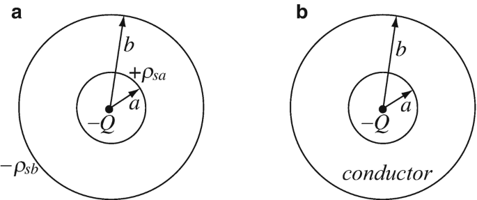
    Figure 4.67

4.1.7 Polarization

• 4.31 Polarization in Dielectrics. Two long, conducting concentric cylindrical shells are separated by two dielectric layers of permittivity ε₁ [F/m] and ε₂ [F/m] as shown in Figure 4.68. A line of charge with line charge density ρ_l [C/m] is placed at the center of the inner shell. Calculate the magnitude and direction of the polarization vector inside the two dielectrics.

  

  Figure 4.68

• 4.32 Polarization in Dielectrics. The space between two large parallel plates, separated a distance d = 0.1 mm, is filled with a dielectric with relative permittivity of 4. The plates are connected to a 12 V battery:

  • (a) What is the electric field intensity in the dielectric?

  • (b) Calculate the polarization vector in the dielectric.

• 4.33 Electric Flux Density in Polarized Medium. A uniform line charge density of ρ_l = 4 μC/m is located along the z axis in free space. A planar surface charge density ρ_s = 20 μC/m² is placed at x = 1, parallel to the y–z plane:

  • (a) Find the electric flux density at a general point P(x,y,z).

  • (b) Find the electric flux density at point P(1,0,0).

  • (c) What is the polarization vector at a general point P(x,y,z), if space has a dielectric constant ε = 4ε₀?

4.1.8 Dielectric Strength

• 4.34 Application: Multilayer Devices. Two parallel plates are connected to a constant electrostatic potential as shown in Figure 4.69. Half the space between the plates is filled with air, one-quarter with a conductor and the fourth quarter with a dielectric with relative permittivity of 80:

  • (a) What is the maximum electric field intensity in the system? Where does this occur?

  • (b) If the breakdown potential in air is 3,000 V/mm and in the dielectric it is 20,000 V/mm, what is the maximum voltage V allowed across the device before breakdown occurs either in air or in the dielectric?

    

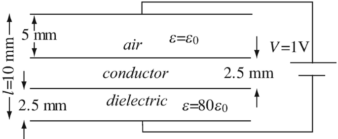
    Figure 4.69

• 4.35 Application: Maximum Charge Density and Maximum Potential on a Sphere. A conducting sphere of radius a [m] is located in air. If the electric field intensity in air cannot exceed 3,000 V/mm:

  • (a) What is the maximum surface charge density the sphere can accumulate?

  • (b) What is the maximum potential that can be connected to the sphere without causing breakdown?

  • (c) What is the maximum possible surface charge density on the surface of planet Earth if its radius is 6370 km and the charge may be assumed to be uniformly distributed on its surface.

• 4.36 Breakdown in Power Lines. A two-conductor power transmission system operates at a voltage V. The radius of each line is 20 mm and the lines are separated a distance of 1 m (between centers):

  • (a) Calculate the maximum voltage difference between the two conductors, V, allowed without causing breakdown. Assume the two lines are charged with equal but opposite sign charge per unit length.

  • (b) If the two lines have an insulation layer made of rubber of thickness 2 mm which has a breakdown voltage much higher than the breakdown voltage in air, what is the estimated maximum voltage allowed now assuming the permittivity of the insulation is close to that of air?

4.1.9 Interface Conditions

• 4.37 Interface Conditions for D. Two dielectric regions are defined by the normal $\hat{\mathbf{n}}=\hat{\mathbf{x}}$ to the interface pointing into region 1. The interface is charge-free. If ε_r = 1, and $\mathbf{E}=\hat{\mathbf{x}}5+\hat{\mathbf{y}}3$ [V/m] in region 1, find the expression for D in region 2 where ε_r = 2.

• 4.38 Interface Conditions on Dielectric Sphere. The electric field intensity inside a dielectric sphere of radius a = 100 mm and relative permittivity ε_r = 12 is given as $\mathbf{E}=\hat{\mathbf{R}}{10}^4{R}^2$ [V/m]. The electric field is generated by an appropriate volume charge density in the dielectric.

  • (a) Calculate the electric field intensity outside the sphere at its surface.

  • (b) Calculate the surface charge density required on the surface of the sphere that will cancel the electric field intensity outside the sphere.

• 4.39 Interface Conditions in Layered Structures. Two flat dielectrics of thickness d [m], both having dielectric constant ε₁ [F/m], are placed on the two sides of a conducting sheet of thickness t [m]. The electric field intensity in free space to the left of the materials is given and is normal to the surface of the dielectric, as shown in Figure 4.70:

  • (a) Calculate the electric field intensity everywhere.

  • (b) What is the potential difference between the left and right surfaces (the potential difference on the three layers)?

    

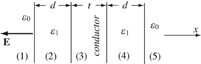
    Figure 4.70

• 4.40 Interface Conditions with Charge Density on the Interface. The electric field intensity in air, in fair weather, is 100 V/m. Suppose the electric field intensity at the surface of the Earth in a flat, desert area points downward and there is a charge density on the surface of –5 × 10^–10 C/m². Assume air has properties of free space and the Earth is a dielectric with relative permittivity of 2:

  • (a) Calculate the electric field intensity immediately below the surface of the Earth.

  • (b) What is the electric field intensity below the surface if the charge density on the surface is zero?

• 4.41 Interface Conditions in Layered Dielectrics. Two large planar layers of dielectric materials are bonded together. An electric field intensity in free space exists to the left of the layers. The layers are each of thickness d [m] (see Figure 4.71):

  • (a) Calculate the electric field intensity everywhere.

  • (b) Calculate the potential difference between two points: one at x = +a [m], the second at x = –a [m].

  • (c) Show that the angle of the electric field intensity in the space to the right of the two layers is θ°.

    

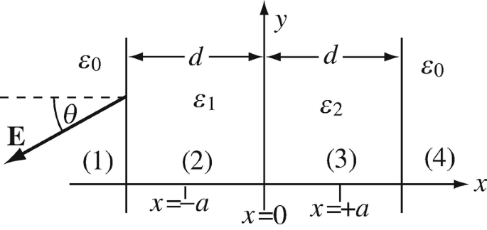
    Figure 4.71

• 4.42 Interface Conditions for the Polarization Vector. Given the interface conditions for the electric field intensity and the electric flux density in Table 4.3:

  • (a) Find the interface conditions required for the polarization vector at the interface between two dielectrics of permittivity ε₁ [F/m] and ε₂ [F/m]. First, assume no free charges on the interface and then allow for existence of free charges on the interface.

  • (b) Determine the ratio of the normal components and the ratio of the tangential components of the polarization vector at the interface between two perfect dielectrics with permittivities ε₁ and ε₂ in terms of the relative permittivity of the two perfect dielectrics. Assume there are no charges at the interfaces.

4.1.10 Capacitance

• 4.43 Application: Parallel Plate Capacitor. A parallel plate capacitor of unit area and separation d [m] is filled with thickness d₁ [m] of a material with ε = 20ε₀ [F/m] and thickness d₂ [m] with a material with ε = 3ε₀ [F/m]. If d₁ + d₂ = d [m], what is the capacitance of the device?

• 4.44 Application: Capacitance per Unit Length of Coaxial Cable. Calculate the capacitance per unit length of the coaxial cable in Figure 4.63.

• 4.45 Application: Spherical Capacitor. Two concentric, conducting spherical shells with radii a = 49 mm and b = 50 mm are separated by a dielectric with relative permittivity ε_r = 3.3. Calculate the capacitance of this device.

• 4.46 Layered Spherical Capacitor. Suppose it is required to double the capacitance of the spherical capacitor of Problem 4.45 by introducing a layer of dielectric material with relative permittivity ε_r = 15, as shown in Figure 4.72. Calculate the thickness of the layer, x:

  • (a) If the layer is placed on the inner shell (Figure 4.72a).

  • (b) If it is placed below the outer shell (Figure 4.72b).

    

    Figure 4.72

• 4.47 Layered Spherical Capacitor. Calculate the capacitance of the device in Figure 4.66.

• 4.48 Application: Capacitance per Unit Length of Coaxial Cable. A coaxial cable is made as shown in Figure 4.73. The inner conductor has radius a [m], the outer conductor has radius b [m]. To separate the two conductors 4 wedges made of a dielectric with permittivity 4ε₀ [F/m] run the length of the cable as shown. Each wedge occupies 30 degrees of the cross section (i.e. 1/12 of the volume between the two conductors). Calculate the capacitance per unit length of the cable.

  

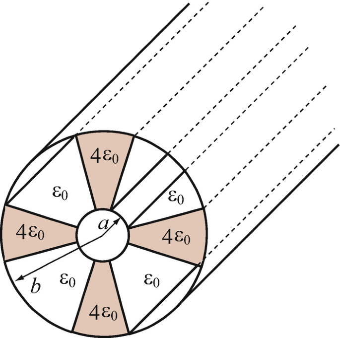
  Figure 4.73

4.1.11 Energy in the Electric Field

• 4.49 Potential Energy of a System of Point Charges. Three point charges are arranged as shown in Figure 4.74. Calculate the potential energy in the system.

  

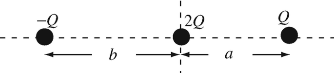
  Figure 4.74

• 4.50 Potential Energy of Distributed Charges. A charged sphere of radius a [m] is charged with a nonuniform volume charge density ρ_v = ρ₀R(R − a) [C/m³], is located in free space, and has permittivity ε [F/m]. Calculate:

  • (a) The energy stored in the volume of the sphere.

  • (b) The energy stored in the space surrounding the sphere.

  • (c) The total energy associated with the sphere.

• 4.51 Energy Stored in a Capacitor. Assume a solid conducting sphere of radius a [m] is connected to a potential V [V] with respect to infinity. Calculate the total energy stored in the electric field produced by the sphere. Assume the charge on the surface of the sphere is uniformly distributed.

• 4.52 Application: Energy and Charge Stored in Parallel Plate Capacitor. A parallel plate capacitor is connected to a voltage source as shown in Figure 4.75a. The dielectric is free space. A flat perfect conductor of thickness a [m] is inserted as shown in Figure 4.75b:

  • (a) What is the change in energy per unit area of the capacitor due to insertion of the conductor (i.e., what is the change in energy for a 1 m² section of the capacitor)?

  • (b) If the capacitor has surface area of 100 mm × 100 mm, d = 1 mm, a = 0.2 mm and is connected to a 12 V source, calculate the total change in charge on the surface of the capacitor as the conductor is inserted assuming the voltage remains unchanged.

  • (c) Repeat (a) and (b) if the conductor is replaced with a dielectric of the same dimensions and a relative permittivity of 4.

  • (d) Describe how this device can be used to detect the conductor (for example, it may be used as a proximity sensor).

    

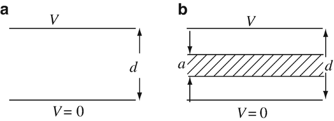
    Figure 4.75

• 4.53 Energy Stored in a Spherical Capacitor. A spherical capacitor is formed by two concentric, conducting shells with a dielectric between them (Figure 4.76). What is the change in stored energy if the dielectric is removed? Assume a known total charge + Q [C] on the inner shell and –Q [C] on the outer shell, and these charges remain constant as the dielectric is removed.

  

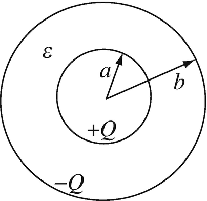
  Figure 4.76

• 4.54 Energy Density. A point charge of magnitude q [C] is located at the center of two concentric, thin spherical shells as shown in Figure 4.77. The inner shell carries a surface charge density ρ₀ [C/m²] and the outer shell a surface charge density –ρ₀ [C/m²]:

  • (a) Calculate the energy density everywhere in space. Plot the energy density.

  • (b) How much energy is stored in the volume between the two shells?

    

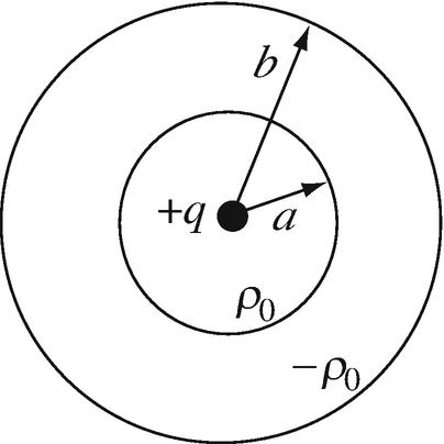
    Figure 4.77

• 4.55 Energy per Unit Length. A line of charge with line charge density ρ_l [C/m] is surrounded by a dielectric layer (filling the space between a and b) as shown in Figure 4.78. The permittivity of the layer is ε [F/m]. Calculate the energy per unit length stored in the dielectric layer.

  

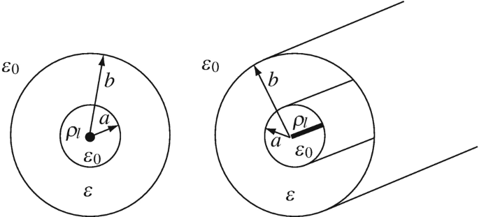
  Figure 4.78

4.1.12 Forces

• 4.56 Application: Pressure in the Electrostatic Field. A parallel plate capacitor with very large plates, separated a distance d [m] apart, is given. The space between the plates is filled with a dielectric with relative permittivity of 2. A potential V [V] is connected across the plates. Assume the distance between the plates is small. Calculate the pressure the plates exert on the material between the plates.

• 4.57 Application: Force in the Electrostatic Field. A square conducting plate, b [m] on the side weighs k [kg], is located over a very large conducting plate, with a dielectric of thickness d [m] and permittivity ε [F/m] between the plates. The plate is connected to a potential V [V] as shown in Figure 4.79 and a string connects it to a weight P [kg]. Neglecting fringing of the electric field, calculate the potential required so that the plate does not move (the weight is balanced by the electrostatic force). The acceleration of gravity is g [m/s²].

  

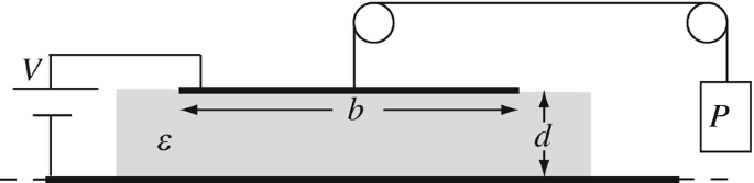
  Figure 4.79

• 4.58 Application: Force in the Electrostatic Field. Two plates, b [m] wide, are separated a distance d [m] apart and overlap a distance c [m] as shown in Figure 4.80. Between the plates there is a dielectric with relative permittivity ε_r. Assume the plates are very close to each other and you can neglect any fringing. A potential V [V] is connected across the plates. Calculate the horizontal force acting on the plates. What is the direction of this force?

  

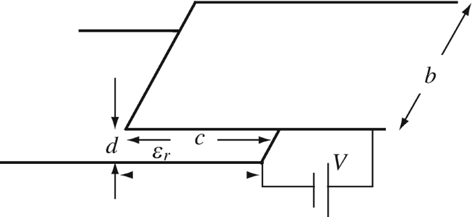
  Figure 4.80

• 4.59 Application: Force on Dielectric in a Capacitor. A parallel plate capacitor is given as shown in Figure 4.81. The dielectric of permittivity ε [F/m] occupies a section of length x [m] and width b [m] between the plates. The rest of the space between the plates is air with a permittivity ε₀ [F/m]. With the dimensions given, calculate the force on the dielectric if a potential difference V₀ [V] exists between the plates. Hint: The force tends to pull the dielectric into the capacitor. If the dielectric were free to move, it would fill the space between the plates.

  

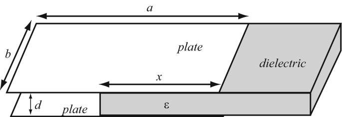
  Figure 4.81

• 4.60 Inflation of a Balloon by Electrostatic Forces. In the early time of space communication, inflatable balloons were used as reflectors to evaluate propagation properties in space. But the use of gas to inflate large space structures is problematic because of leaks, diffusion across the structure skin, and finite supply. A possible alternative is to use charge and the forces it can generate to keep the structure “inflated” without the need for gas. Since charge can be generated as needed using harvested energy through solar cells, the structure can maintain its shape indefinitely. Consider a balloon of radius a [m], charged with a surface charge density ρ₀ [C/m²] in free space:

  • (a) Calculate the pressure inside the balloon.

  • (b) What is the required charge density for a balloon of radius 10 m if the pressure required is 100 pascals (Pa). (1 pascal = 1 N/m²)?

  • (c) If the maximum electric field intensity that can be generated is 10⁹ V/m, what is the maximum pressure achievable using the dimensions in (b)?